Abstract

Linear response functions are calculated for symmetric nuclear matter of normal density by time-evolving two-time Green’s functions with conserving self-energy insertions, thereby satisfying the energy-sum rule. Nucleons are regarded as moving in a mean field defined by an effective mass. A two-body effective (or residual) interaction, represented by a gaussian local interaction, is used to find the effect of correlations in a second order as well as a ring approximation. The response function $S(\omega,q)$ is calculated for $0.2<q<1.2fm^{-1}$. Comparison is made with the nucleons being un-correlated, ”RPA+HF” only.

1 Introduction

This report concerns the calculation of the density response function in symmetric nuclear matter when subjected to an external probe. This problem has traditionally involved solving a Bethe-Salpeter equation. A main problem with that method is the construction of a consistent interaction kernel, to satisfy the energy sum-rule. Such a calculation was however accomplished by Bozek for nuclear matter[1] and further applied in ref.[2] Response functions have of course since long been the focus of intense studies for the electron gas with numerous contributions. Early works by Lundqvist and Hedin are noticeable leading to the often cited GW method. [3] More recent works include those of Faleev and Stockman focussing on electrons in quantum wells.[4]

An alternative method, first applied by Kwong and Bonitz for the plasma oscillations in an electron gas, is a real time solution of the Kadanoff Baym equations.[5] With conserving approximations of the two-time Green’s functions the energy sum rule is automatically guaranteed. The details of this method was already presented in the paper by Kwong and Bonitz. The main purpose here is to illustrate this method for the calculation of response functions in symmetric nuclear matter, emphasizing the relative ease of these computations and also the relation of these calculations to the nuclear many-body problem in general.

It was shown in Baym and Kadanoff’s original papers [6] that, if one wishes to construct the linear response function from dressed equilibrium Green’s functions, appropriate vertex corrections to the polarization bubble are necessary to guarantee the preservation of the local continuity equation for the particle density and current in the excited system, which in turn implies the satisfaction of the energy-weighted sum rule. This condition is satisfied if the appropriate selfenergies are calculated in a conserving approximation.

2 Formalism

Symmetric nuclear matter is subjected to an external perturbation specified below. Nucleons are initially at time $t=0$ assumed to be uncorrelated but moving in a mean field defined by an effective mass $m^{*}$. The initial temperature is usually assumed to be $T=0$, but in some cases shown below it is assumed to be 20 MeV. In those cases where the effect of correlations is studied an interaction which is local (in coordinate space) is switched on and the system is time-evolved in real time until fully correlated, at $t=10fm/c$. As a consequence of the conserving approximations the system will during this time heat up. The external perturbation is now turned on and the system will exhibit density-fluctuations in time. Details are presented below.

2.1 The two-time KB-equations

The Kadanoff-Baym equations in the two-time form for the specific problem at hand was already shown in previous work, where it was applied to the electron gas.[5] Few modifications are necessary for the present nuclear problem.

We consider three separate cases:
I. Uncorrelated, mean field only, HF+RPA approximation.
II. Correlations included by second order self-energies with a residual interaction, eq.(17) below.
III. Ring-diagrams included in the selfenergy to all orders.
The selfenergy obtained with the second order Born approximation as well as RPA are ’conserving approximations’. [6]

As made clear in ref. [5] there is no separate need to calculate vertex corrections. They are generated by the time-evolution of the Green’s functions.

The Green’s function is separated into a spatially homogeneous part $G_{00}$ and a linear response part $G_{01}$.

Calculations proceed as follows: Equilibrium Green’s functions are constructed for an uncorrelated fermi distribution of specified density and temperature. These $G_{00}$ functions are time-evolved with the chosen mean field and correlations (I,II or III above) until stationary. (typically $10fm/c$). An external field $U_{0}(t)$ is then applied which generates particle-hole functions $G^{{}^{>}_{<}}_{10}$ propagated by eqs (6) in ref[5]. They are for completeness repeated here

$$\left(i\hbar\frac{\partial}{\partial t}-\epsilon_{{\bf k+q_{0}}}\right)G_{10}^{{}^{>}_{<}}({\bf k}tt^{\prime})=U_{0}(t)G_{00}^{{}^{>}_{<}}({\bf k}tt^{\prime})+\Sigma_{1m}^{HF}({\bf k}t)G_{m0}^{{}^{>}_{<}}({\bf k}tt^{\prime})$$

$$+\Sigma_{1m}^{R}({\bf k}t\bar{t})G_{m0}^{{}^{>}_{<}}({\bf k}\bar{t}t^{\prime})+\Sigma_{1m}^{{}^{>}_{<}}({\bf k}t\bar{t})G_{m0}^{A}({\bf k}\bar{t}t^{\prime})$$ (1)

and

$$\left(-i\hbar\frac{\partial}{\partial t^{\prime}}-\epsilon_{{\bf k}}\right)G_{10}^{{}^{>}_{<}}({\bf k}tt^{\prime})=U_{0}(t^{\prime})G_{11}^{{}^{>}_{<}}({\bf k}tt^{\prime})+G_{1m}^{{}^{>}_{<}}({\bf k}tt^{\prime})\Sigma_{m0}^{HF}({\bf k}t^{\prime})$$

$$+G_{1m}^{R}({\bf k}t\bar{t^{\prime}})\Sigma_{m0}^{{}^{>}_{<}}({\bf k}\bar{t}t^{\prime})+G_{1m}^{{}^{>}_{<}}({\bf k}t\bar{t^{\prime}})\Sigma_{m0}^{A}({\bf k}\bar{t}t^{\prime})$$ (2)

the selfenergies $\Sigma_{00}$ are given by

$$\Sigma_{00}^{{}^{>}_{<}}({\bf k},t,t^{\prime})=i\sum_{\bf p}G_{00}^{{}^{>}_{<}}({\bf k-p},t,t^{\prime})V_{s}^{{}^{>}_{<}}({\bf p},t,t^{\prime}).$$ (3)

In the second order calculautions (case II) we have

$$V_{s}^{{}^{>}_{<}}({\bf p},t,t^{\prime})=V^{2}({\bf p})\Pi_{00}^{{}^{>}_{<}}({\bf p},t,t^{\prime})$$ (4)

where $V({\bf p})$ is the momentum-representation of the residual potential, local in ccordinate space, eq. (17).

The polarisation bubble $\Pi_{00}$ is defined by

$$\Pi_{00}^{{}^{>}_{<}}({\bf p},t,t^{\prime})=-i\sum_{\bf p^{\prime}}G_{00}^{{}^{>}_{<}}({\bf p^{\prime}},t,t^{\prime})G_{00}^{{}^{<}_{>}}({\bf p^{\prime}-p},t^{\prime},t)$$ (5)

The selfenergies in the (10) channel are given by

$$\Sigma_{10}^{{}^{>}_{<}}({\bf k},t,t^{\prime})=i\sum_{\bf p}[G_{10}^{{}^{>}_{<}}({\bf k-p},t,t^{\prime})V_{s}^{{}^{>}_{<}}({\bf p},t,t^{\prime})$$

$$+G_{00}^{{}^{>}_{<}}({\bf k-p},t,t^{\prime})V_{s(10)}^{{}^{>}_{<}}({\bf p},t,t^{\prime})]$$ (6)

with

$$V_{s(10)}^{{}^{>}_{<}}({\bf p},t,t^{\prime})=V^{2}({\bf p})\Pi_{10}^{{}^{>}_{<}}({\bf p},t,t^{\prime})$$ (7)

and the polarisation bubble in the $(10)$-channel is given by

$$\Pi_{10}^{{}^{>}_{<}}({\bf p},t,t^{\prime})=-i\sum_{\bf p^{\prime}}[G_{10}^{{}^{>}_{<}}({\bf p^{\prime}},t,t^{\prime})G_{00}^{{}^{<}_{>}}({\bf p^{\prime}-p},t^{\prime},t)$$

$$+G_{00}^{{}^{>}_{<}}({\bf p^{\prime}},t,t^{\prime})G_{10}^{{}^{<}_{>}}({\bf p^{\prime}-p-q},t^{\prime},t)]$$ (8)

In case III where not only the second order but all RPA-rings are included in the selfenrgies one has

$$V_{s}^{{}^{>}_{<}}({\bf p},t,t^{\prime})=V({\bf p})[\int_{t_{0}}^{t}dt^{\prime\prime}(\Pi_{00}^{>}({\bf p},t,t^{\prime\prime})-\Pi_{00}^{<}({\bf p},t,t^{\prime\prime}))V_{s}^{{}^{>}_{<}}({\bf p},t^{\prime\prime},t^{\prime})-$$

$$\int_{t_{0}}^{t^{\prime}}dt^{\prime\prime}\Pi^{{}^{>}_{<}}({\bf p},t,t^{\prime\prime})(V_{s}^{>}({\bf p},t^{\prime\prime},t^{\prime})-V_{s}^{<}({\bf p},t^{\prime\prime},t^{\prime}))]+$$

$$V^{2}({\bf p})\Pi_{00}^{{}^{>}_{<}}({\bf p},t,t^{\prime})$$ (9)

and

$$V_{s(10)}^{{}^{>}_{<}}({\bf p},t,t^{\prime})=\int_{t_{0}}^{t}d\bar{t}\int_{t_{0}}^{t^{\prime}}d\bar{t^{\prime}}$$

$$\{V_{s}^{R}({\bf p+q},t,\bar{t})\Pi_{10}^{R}({\bf p},\bar{t},\bar{t^{\prime}})V_{s}^{{}^{>}_{<}}({\bf p},\bar{t^{\prime}},t^{\prime})$$

$$+V_{s}^{R}({\bf p+q},t,\bar{t})\Pi_{10}^{{}^{>}_{<}}({\bf p},\bar{t},\bar{t^{\prime}})V_{s}^{A}({\bf p},\bar{t^{\prime}},t^{\prime})$$

$$+V_{s}^{{}^{>}_{<}}({\bf p+q},t,\bar{t})\Pi_{10}^{A}({\bf p},\bar{t},\bar{t^{\prime}})V_{s}^{A}({\bf p},\bar{t^{\prime}},t^{\prime})\}$$ (10)

where the retarded and advanced parts are given by

$$\Sigma_{10}^{R/A}({\bf p},t,t^{\prime})=\pm\theta(\pm(t-t^{\prime})[\Sigma_{10}^{>}({\bf p},t,t^{\prime})-\Sigma_{10}^{<}({\bf p},t,t^{\prime})]$$ (11)

$$\Pi_{10}^{R/A}({\bf p},t,t^{\prime})=\pm\theta(\pm(t-t^{\prime})[\Pi_{10}^{>}({\bf p},t,t^{\prime})-\Pi_{10}^{<}({\bf p},t,t^{\prime})]$$ (12)

$$V_{s}^{R/A}({\bf p},t,t^{\prime})=\delta(t-t^{\prime})V({\bf p})\pm\theta(\pm(t-t^{\prime})[V_{s}^{>}({\bf p},t,t^{\prime})-V_{s}^{<}({\bf p},t,t^{\prime})]$$ (13)

The Hartree-Fock selfenergy in the ($00$)-channel is approximated by an effective mass $m^{*}=0.7m$. In the ($10$)-channel it is given by

$$\Sigma_{10}^{HF}({\bf p},t)=-iV(q)\sum_{\bf p^{\prime}}G^{<}_{10}({\bf p^{\prime}},t,t)+i\sum_{\bf p^{\prime}}G^{<}_{10}({\bf p-p^{\prime}},t,t)V(p)$$ (14)

The second term, the Fock-term, was found to be negligent and subsequently omitted in calculations. The Hatree-term on the other hand is what drives the fluctuations in the response function.

The eqs. (1) and (2) are time-evolved and the response-function is, after fourier-transformations of $G^{<}_{10}({\bf p},t,t)$ and $U_{0}(t)$ with respect to time t, calculated from

$$S(\omega,q)=\frac{1}{\pi n_{0}U_{0}(\omega)}\sum_{\bf p}ImG^{<}_{10}({\bf p},\omega)$$ (15)

$U_{0}(t)$ was chosen to be a Gaussian with a width of $3fm/c$.

2.2 Interactions

The outcome of any microscopic many-body calculation depends on the assumption of the interactions between the individual particles. Some information on the NN- interaction betewen two nucleons in free space is obtained from scattering. It is however incomplete being only on-shell. Some off-shell information can be obtained indirectly from bound nuclei e.g. the deuteron. It has to be complemented by theoretical input the most important of which is the OPEP. It does however lack information on experimentally known short-ranged repulsions and has to be augmented by contributions from heavier exchange particles.[8] There is also the question of contributions from not only 2- but also 3- (and higher) body forces. This is ongoing research that leaves any present nuclear many-body calculation open for future modifications.

With interactions given one can (at least in principle) calculate properties of the 3-nucleon system as well as those of light nuclei ”exactly” by Faddeev or no-core shell-model techniques. More generally there is however the question of an acceptable many-body theory. Many-body theories usually assume the importance of specifis terms (diagrams) in some (sometimes unspecified) expansion resulting in some in-medium interaction such as Brueckner’s Reaction mtarix.

The theoretical problem of nuclear structure is consequently two-fold.
I. Construction of N-N (as well as N-N-N etc) interactions.
II. A many body theory allowing the calculation of nuclear properties.
There has been much progress relating to both of these problems during the last more than 50 years of nuclear research but ongoing studies are still intense and of course facilitated by development of computers. We are here not implementing the full machinery of these findings but will use the provided knowledge to model the nuclear properties. This is of course what is mostly done in this kind of work. Examples are the Skyrme and Gogny forces. We shall model the symmtric nuclear matter under consideration here as a system of particles (nucleons) with masses $m$ moving in a momentum dependent (Hartree-Fock) mean field interacting with an in-medium effective 2-body interaction. In general such an interaction would be given in momentum-space by:

$$<{\bf k}|K|{\bf k^{\prime}}>\equiv K({\bf p,q})$$ (16)

where ${\bf p}=({\bf k+k^{\prime}})/2$ and ${\bf q=k-k^{\prime}}$. As a result of the effective interaction being non-local (in coordinate space) the diagonal Hartree-Fock (or ”Brueckner Hartree-Fock”) mean field is momentum-dependent which is very important. We therefore approximate $\Sigma^{HF}_{00}$ by introducing an effective mass $m^{*}=0.7m$.

In order to find the effect of 2-body correlations between the nucleons moving in this mean field we approximate the in-medium K-matrix by a simplified ’residual’ interaction, often used in this context[9, 2, 10]. It is local in coordinate space. In momentum-space it reads:

$$V({\bf q})=\pi^{3/2}\eta^{3}V_{0}e^{-\frac{1}{4}\eta^{2}q^{2}}$$ (17)

with $\eta=0.57{\rm fm}$ and $V_{0}=-453$ MeV.

Notice that this interaction only depends on the ’transverse’ momentum $q$ in momentum space but not on the momentum $p$, responsible for the concept of an effective mass. It would therefore not be adequte for building the diagonal Hartree-Fock field $\Sigma^{HF}_{00}$ specified above.

The (off-diagonal) $q$-dependence of the effective interaction is however important in the context of the present investigation where the response is in fact ”driven” by the Hartree-term in eq. (14). It is unfortunately less accessible wheras the diagonal is more closely related to the scattering $T$-matrix. We shall here use the interaction (17) in the Hartree term of eq. (14) and for evaluating the correlation terms.

There is no inconsistency in the two choices, the one for the mean field and the one for correlations. They are just two aspects of the sam effective interaction.

Other possible choices would have been any of the family of Skyrme- or Gogny-forces which have been used in other works related to the nuclear response function. They allow for the spin-isospin dependence of the response, lacking in our choice. Specific features of the interaction such as tensor[11] and pairing[12] have been investigated.

The main purpose of the present work is for illustration of the 2-time method. Our simple choices for the interaction fulfills this purpose.

2.3 Equilibrium Temperature

In a KB-calculation, with the selfenergy defined by a conserving approximation the total energy is conserved. Assuming, as in the present work, that the system is initially un-correlated the potential energy will decrease the and kinetic energy will increase with the same amount until the system is fully correlated and internal equilibrium is reached. The result is an increase in temperature from the initially set value. This situation can be moderated by an imaginary time-stepping method. The final, equilibrated,temperature $T_{f}$ will then be a function of the initial imaginary time $\tau$ with $T_{f}=0$ in the limit where $\tau\rightarrow\infty$.

For finite values of $\tau$ this final equilibrium temperature $T_{f}=1/\beta$ and chemical potential $\mu$ is obtained from the following relation between $\Sigma^{<}$ and $\Sigma^{>}$ (valid at equilibrium) [7]:

$$\Sigma^{>}({\bf p},\omega)=-e^{\beta(\omega-\mu)}\Sigma^{<}({\bf p},\omega).$$ (18)

Note that, as a consequence of eq. (18), the ratio of the selfenergies is independent of momentum ${\bf p}$, which serves as a check on numerical accuracy and that equilibrium has been reached.

With $\beta$ and $\mu$ given the equilibrium uncorrelated distribution function is given by

$$f(p)=1/(1+e^{\beta(\omega(p)-\mu)})$$ (19)

with

$$\omega(p)=p^{2}/2m+Re\Sigma^{+}({\bf p},\omega)+\Sigma^{HF}(\bf p)$$ (20)

The real part of $\Sigma^{+}$ is obtained from the imaginary part by the dispersion relation, after using the relation

$$2Im\Sigma({\bf p},\omega)=i(\Sigma^{<}({\bf p},\omega)-\Sigma^{>}({\bf p},\omega)$$ (21)

While the uncorrelated distribution is given by eq. (19) the correlated is different, and given by

$$\rho({\bf p},t)=-iG^{<}({\bf p},t,t).$$ (22)

The diffence between these two distributions is important. If for example the initial temperature is zero in which case $f(p)$ has a sharp cut-off at the fermi-surface, the correlated distribution $\rho({\bf p})$ is ’smoothed’ at the surface. The available phase-space for excitations differs.

Fig. 1 shows the temperature as a function of imaginary time $\tau$, as calculated with the equations above.

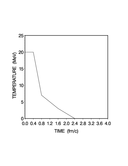
Figure 1: The temperature as a function of imaginary time $\tau$. See text for details.

3 Numerical results

Calculations are made for symmetric nuclear matter at normal nuclear matter density, $\rho=0.16fm^{-3}$ and some selected temperatures $T$. The external momentum transfer is chosen to be $0.2<q<1.2fm{-1}$. The computing method that we used was mainly as is described in ref. [13] with the additional requirement to also time-evolve $G_{01}$.[5] The fluctuating density

$$\delta n(q,t)=-\sum_{p}G^{<}_{10}(p,t,t)$$

is recorded until fully damped. If the damping time is too large (number of time-steps $>\sim 150$) then $n(q,t)$ is extrapolated using the amplitudes and frequencies of the oscillations for lesser times. A typical result of the evolution in real time and an extrapolation is shown in Fig 2, including also the quadrupole deformation in momentum-space.

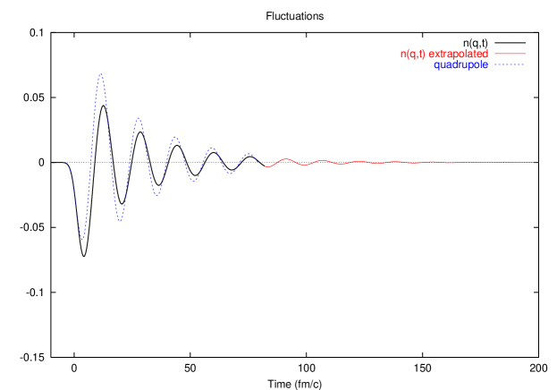
Figure 2: Solid curve shows the fluctuating density as a function of time. It is in this particular case extrapolated for times $t>82fm/c$ (red online). The broken curve (blue online) shows the associated quadrupole-moment of the deformation in momentum-space.

This time-function is then fourier-transformed to $\omega$-space.

Results for the three different situations referred to in the Introduction are shown below.

3.1 Mean field +RPA; case I

The mean field is here included in an effective mass approximation with $m^{*}=0.7$, all correlations are neglected, i.e. all selfenergies (except the HF) are identically zero. Fig 3 show results at zero and 20 MeV temperature for three different values of $q$.

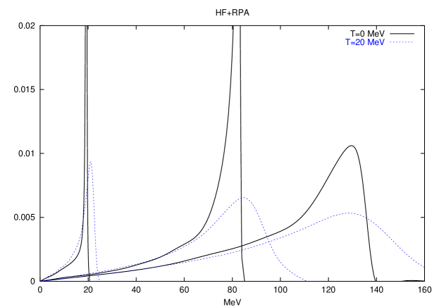
Figure 3: Response functions $S(\omega,q)$ in the HF+RPA approximation. Solid curves show results at zero temperature for external momentum transfers $q=0.2,0.8$ and $1.2fm^{-1}$ respectively. Broken curves (blue online) show results when temperature is raised to 20 MeV.

A sharp resonance is found for the smallest value of $q=0.2fm^{-1}$ at temperature $T=0$. Notable is the sharp cut-off on the high $\omega$-side. (compare ref. [14]). The width increases as $q$ approaches the fermimomentum but the sharp cut-off persists. With the temperature increased to T=20 MeV this sharp cut-off is eliminated and the widths at all values of $q$ is also increased.

3.2 $2^{nd}$ order correlations; case II

The Green’s functions are in this section dressed by second order insertions as outlined above with the interaction given by eq. (17).

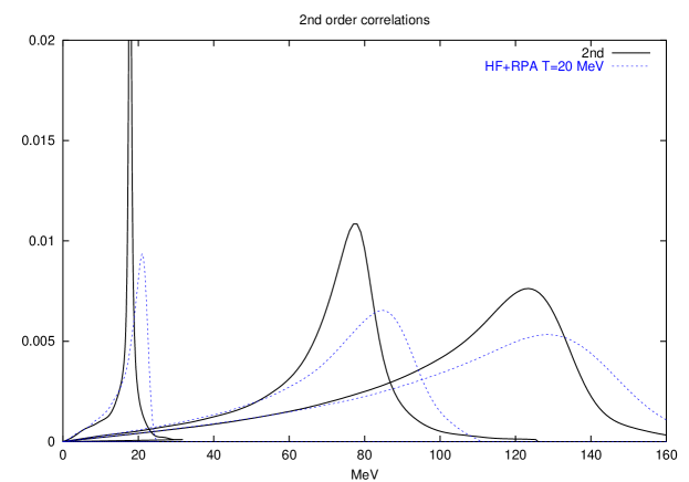
Figure 4: Solid curves show response functions $S(\omega,q)$ with $2^{nd}$ order correlations included. External momentum transfers are $q=0.2,0.8$ and $1.2fm^{-1}$ respectively. They are compared with HF+RPA results at temperatures T=20 MeV: broken curves (blue online). See text for further explanations.

The initial temperature, at time $t=0$ is here equal to zero, the momentum-distribution is that of a zero-temperature fermi-distribution. After the system is fully correlated (for times $t>t_{c}$), the temperature will as described above, have increased. Referring to Fig.1 this temperature is estimated to be 20 MeV. In the linear response limit that is used here, separating the Green’s function into $G_{00}$ and $G_{01}$ components, the collision term for the $G_{00}$ evolution will be zero for $t>t_{c}$. The external momentum perturbation is applied at this time. With the conserving approximation satisfied the vertex-correction is ’automatically’ included.[5] Results of these calculations are shown in Fig. 4 for three different values of the external momentum transfer $q$. Comparing with the zero temperature results in Fig. 3 one finds no appreciable shift in resonance energies but a small broadening that increases with $q$. The sharp cut-offs at the high energy tails are replaced by smoother tails, somewhat similar to what is seen in Fig. 3 at T=20 MeV. One effect associated with the correlations is a smoothing of fermi-surface somewhat similar to that of a temperature increase. This is of course a consequence of the broadening of the static spectral functions caused by the imaginary parts of the self-energies.

3.3 Full Ring-correlations; case III

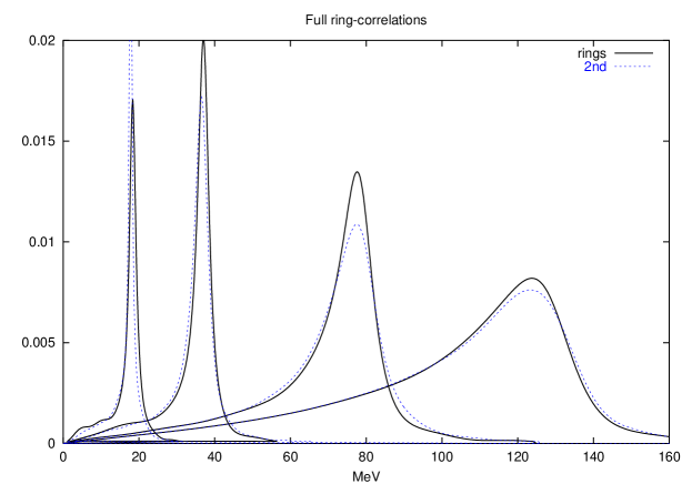
Figure 5: Solid curves show response functions $S(\omega,q)$ with full ring correlations included for external momentum transfers $q=0.2,0.4,0.8$ and $1.2fm^{-1}$ respectively. They are compared with $2^{nd}$ order results: broken curves (blue online). See text for further explanations.

The results above, showing the effect of including correlation to second order in the chosen interaction is here extended with the inclusion of polarisation bubbles to all orders. This seems a logical extension of the second order which after all is just the lowest order of the full ring expansion. This is of course well known to be of extreme importance in the theory of the electron gas, providing screening. Fig. 5 shows our result. The difference from the $2^{nd}$ order, that is shown by the broken line, is seen to be small. Only a slight sharpening of the resonances is observed.

4 Summary and Conclusions

The main purpose of this presentation is to illustrate the usefulness of the two-time Green’s function (Kadanoff-Baym) method for the study of nuclear response. It was previously applied to the electron gas to see the effect of correlations.[5] The time-evolution of Green’s function in two-time space with conserving approximations for the self-energies guarantees the preservation of sum-rules. An alternative method, the solution of the Bethe-Salpeter (BS) equation (in $\omega$-space) has been carried through by Bozek et al.[1, 2]. It is found that zero temperature and/or small $q$ calculations, where the spectral width is small, present numerical problems when using this BS-formalism.

This is not a problem when using the present method with the two-time Green’s functions.

The rise in temperature associated with the onset of correlations when using the two-time method is sometimes cited as a drawback. It is however not difficult to remedy by allowing the correlations to proceed in the imaginary time-domain. It requires of course to have access to the proper computer-codes. It is our aim to utilise these existing codes in future work.

Comparing the results obtained so far in our on-going investigation one does not find any major difference in the three different approximations, collisionless, $2^{nd}$-order or full rings. In this regard our result agrees with those of ref. [2].

The method of two-time Green’s function time-evolution is well documented, but there are certainly improvements in its application to the problem of nuclear response that are desired. Most of these are common with any nuclear many body problem such as NN-forces and in-medium effects. Although our understanding of nuclear forces and of the nuclear many-body problem is under constant development it is till incomplete. There is however important knowledge that can and should be incorporated in future nuclear response calculations. Spin-isospin, tensor and pairing are all aspects of the interaction that have already been shown to be of interest[2, 11, 12] and still remain to be included in our calculations.

The results shown are for symmetric nuclear matter. Response calculations for neutron matter is of particular interest related to astrophysical problems.

The local interaction that has been used to find the effect of correlations may be adequate but a more ”realistic” non-local,state-dependent, interaction should be used. Separable interactions have been developped from inverse scattering that can easily be incorporated in our calculations. The long-range ($V_{low-k}$) version of these would be adequate. It has already ben shown that as far as the spectral width concerns it is indeed the long-ranged part that plays the important role.[15] The self-energy insertions have been separated into a Hartree-Fock (mean field) that is real and a ’correlation’ part which is complex. This can be done consistently in the case of weak interactions. With medium-dependent effective interactions such a separation is not well defined and can lead to double-counting. In the present work the mean field is assumed to be included by an effective mass that could for example be the result of a Brueckner calculation involving a summation of ladder diagrams and more. The real part of the second order self-energy insertion used to find the effect of correlations would therefore already be included in a Brueckner mean field. So one may claim that a double-counting has been done. The main objective of the second order insertion is however to find the effect of the broadening of the spectral-function and this is a consequence of the insertion having an imaginary part and, as mentioned, this imaginary part stems mainly from the long-ranged part of the interaction. As a result we claim that the important physics is (reasonably well) incorporated in our calculations. Future work should however address this point in a fully consistent way. More important is however a fully consistent calculation of the $q-dependent$ Hartree field that is the driving mechanism of the response. It was derived from the same local interaction as for the second order selfenergy. An better alternative would be for example to use the Brueckner $K$-matrix as outlined above in the Introduction.

5 Acknowledgements

One of us (HSK) wishes to thank The University of Arizona and in particular the Department of Physics for providing office space and access to computer facilities. This work has not been supported by any external agency.

References

- [1] P. Bozek, Phys. Letters B579 309 (2004).
- [2] P. Bozek,J. Margueron and H. Müther, Ann. Phys.(N.Y.) 318 245 (2005).
- [3] L. Hedin and S. Lundqvist, Solid State Physics (Acadenmic, New York, 1969) Vol 23.
- [4] Sergey V. Faleev and Mark.I. Stockman Phys. Rev.B 63 193302 (2001), Phys. Rev.B 66 085318 (2002).
- [5] N. H. Kwong and M. Bonitz, Phys. Rev. Letters 84 1768 (2000).
- [6] Gordon Baym and Leo P. Kadanoff, Phys. Rev. 124 287 (1961) ; Gordon Baym, Phys. Rev. 127 1391 (1962).
- [7] L.P. Kadanoff and G.Baym, Quantum Statistical Mechanics. (Benjamin,New York, 1962).
- [8] R. Machleidt and D.R. Entem, Physics Reports 503 1 (2011).
- [9] P. Danielewicz, Ann. Phys.(N.Y.) 152 305 (1984).
- [10] H.S. Köhler, Phys. Rev.C 51 3232 (1995).
- [11] E. Olsson, P. Haensel and C.J. Pethick, nucl-th/0403066, G.I. Lykasov, E. Olsson and C.J. Pethick, nucl-th/0502026
- [12] Armen Sedrakian and Jochen Keller, nucl-th/1001.0395 Jochen Keller and Armen Sedrakian nucl-th/1205.6902
- [13] H.S. Köhler, N.H. Kwong and Hashim A. Yousif, Comp.Phys.Comm. 123 123 (1999).
- [14] J. Margueron, Ngguyen Van Giai and J. Navarro, nucl-th/0507053
- [15] H.S. Köhler Nucl. Phys. 88 529(1966)