On the Security of Key Extraction from Measuring Physical Quantities

Abstract

Key extraction via measuring a physical quantity is a class of information theoretic key exchange protocols that rely on the physical characteristics of the communication channel, to enable the computation of a shared key by two parties that share no prior secret information. The key is supposed to be information theoretically hidden to an eavesdropper. Despite the recent surge of research activity in the area, concrete claims about the security of the protocols typically rely on channel abstractions that are not fully experimentally substantiated. In this work, we propose a novel methodology for the experimental security analysis of these protocols. The crux of our methodology is a falsifiable channel abstraction that is accompanied by an efficient experimental approximation algorithm of the conditional min-entropy available to the parties given the view of the eavesdropper.

We focus on the signal strength between two wirelessly communicating transceivers as the measured quantity and we use an experimental setup to compute the conditional min-entropy of the channel given the view of the attacker which we find to be linearly increasing. Armed with this understanding of the channel, we showcase the methodology by providing a general protocol for key extraction in this setting that is shown to be secure for a concrete parameter selection. In this way we provide a comprehensively analyzed wireless key extraction protocol that is demonstrably secure against passive adversaries assuming our falsifiable channel abstraction. Our use of hidden Markov models as the channel model and a dynamic programming approach to approximate conditional min-entropy might be of independent interest, while other possible instantiations of our methodology can be feasible and may be motivated by this work.

I Introduction

Key extraction between two parties, Alice and Bob, by measuring a physical quantity is based on two basic premises. First, due to the physical properties of the quantity measured, Alice and Bob obtain highly correlated measurements. Second, the measurements obtained by the eavesdropper are weakly correlated. This hypothesized gap of the correlation of measurements between Alice and Bob and the correlation of the eavesdropper’s measurements opens the door for a key exchange mechanism that would have to perform an information reconciliation [1] and privacy amplification [2] step to enable the calculation of a secret key that is almost independent of the adversary’s view.

In the literature, one can distinguish two classes of such protocols. The first class is practice-oriented protocols in which the security of the key follows directly from certain strong assumptions or is based (at best) on statistical tests. The second class is theoretical protocols in which broad channel abstractions are made and then these are formally shown to imply a correlation gap between the adversary and the two parties, thus showing information theoretic security. Nevertheless, despite that security is proven formally, for a real-world implementation, a leap of faith is still required to accept the fact that the channel abstraction is indeed capturing the real-world setting of the adversary. The only exception is quantum key-exchange, where there are results from quantum mechanics such as the no-cloning theorem that do provide the underlying formal basis justifying the connection between the channel abstraction and the real-world. The lack of strong general arguments in key extraction from measuring physical quantities means that any deviation of the real-world adversary setting from the assumed channel abstraction will lead to a security breakdown and thus to a dubious security status for the key extraction protocol.

In this work we take a first step towards addressing this fundamental problem by providing a novel formal security methodology that enables us to argue experimentally about the security of such protocols. In a nutshell, we put forth a general framework that (i) enable us to mathematically estimate the conditional entropy in the key extracted from physical measurements; (ii) the security arguments can be tied to a specific real-world setting through falsifiable (but not oversimplified) assumptions.

I-A Related Work and Our Results

Information-theoretic treatment of secure key exchange was initiated by Wyner [3] in the wiretap model and it was later studied by Maurer [4] and Ahlswede, Csiszar [5] in the common random source model. These works dealt with the feasibility of key exchange assuming a non-zero “equivocation-rate”, a measure expressing the uncertainty of the eavesdropper about the parties’ communication. Beyond generic schemes, for specific physical quantities, there has already been a series of theoretical studies, in quantum key exchange [6], and wireless key exchange focusing on the “secrecy capacity” between wirelessly communicating transceivers, (e.g., [7], following the wiretap channel and [8, 9, 10, 11, 12, 13, 14], following the shared randomness channel.) These works, being conceptual only [13, 14], or information theoretic in nature, contain no experimental justification of the channel model they utilize: for the quantum ones, the underlying physics justify the model but the wireless ones have no real-world justification, most of them relying on the assumption that the signal measurements are independent across time and thus any existing non-zero equivocation rate can be magnified for a suitable number of transmissions straightforwardly.

Considering works that were more experimental in nature, there were several practical algorithms suggested for wireless key extraction  [15, 16, 17, 18, 19, 20, 21, 22, 23, 24, 25]. A common characteristic of these works is that significant attention is given to demonstrate correctness (i.e., that Alice and Bob calculate the same key), and efficiency; much less formal analysis (as we detail below) is performed to demonstrate security. More specifically, the security of many of these works, e.g., [23, 16, 18, 19], directly relied on the assumption that if the adversary is a wavelength away from the communicating parties, the adversary’s observation is independent of the parties’ measurements. Some other works made some further steps to analyze security. For instance, [23, 24] consider performing randomness tests but these are insufficient as security guarantees (such “random” sequences are not necessarily unpredictable). In [20] a type of attacks based on blind deconvolution is considered and it is argued experimentally that such attacks are unlikely to apply; however, this does not preclude other types of attacks. Works such as [22, 17] provided informal security arguments based on calculating the correlation between the eavesdropper’s measurements and the parties’ measurements. However, such correlation calculation can not guarantee the amount of (conditional) entropy contained in the extracted key.

In fact, the lack of properly rigorous security claims can lead to (partial) key recovery attacks as demonstrated in [26, 27] that examined known protocols in a specific deployment. These works exemplified the fact that even though existing analysis has demonstrated successfully that the signal observed by the two parties has sufficient entropy it remains open whether the conditional entropy on the eavesdropper’s view is non-zero in a specific real-world deployment.

A number of techniques for reconciling the errors between the two communicating parties have been shown in the literature. For real valued measurements (as in the wireless key exchange setting), a popular approach employs a “thresholding” methodology [17, 23] where the signal is transformed to a bitstring using only the level of measurements where, for example, deep fades are observed. In such settings it can be shown that the errors are so few that reconciliation becomes easy. Unfortunately, such reconciliation requires interaction that may result in potentially zeroing the conditional entropy, a fact that experimentally remains open. Other approaches suffer from similar problems, such as [16] that relies on the Cascade protocol or [22] that uses specialized antennas.

We conclude that information theoretic security in all these previous works relies on whether the channel abstraction fits the real-world adversary setting and whether any additional reconciliation interaction performed does not cut from the conditional entropy too much. While ad hoc lower bound assumptions on the conditional entropy of Alice and Bob’s measurements given the view of the adversary are sufficient to argue the security of the key, it is very hard to experimentally verify that such assumptions are indeed true. Indeed, in order to apply the textbook calculation of conditional entropy, one would have to carry experiments an immense number of times. Even worse, one can formally prove that an exponential number of samples are necessary for approximating conditional entropy in the general case (this can be derived from [28]).

In this work we address the above problems with the following contributions.

• First, we introduce a methodology to experimentally argue about the security of key exchange protocols that are based on measuring real-valued physical quantities in the passive model: The crux of our methodology is a falsifiable channel abstraction that is accompanied by an efficient experimental approximation algorithm of the conditional min-entropy of the two parties given the view of the eavesdropper.

  Specifically, we model measurements and adversarial observations via a hidden Markov model (HMM) and we utilize a dynamic programming approach to estimate the conditional min-entropy : we achieve that through a combination of the Viterbi algorithm [31] and the forward algorithm [32]. This algorithmic approach is beneficial as it allows with only a polynomial number of experiments in the size of the key to argue about the conditional min-entropy without oversimplifying the channel abstraction (e.g., assuming measurements are mutually independent across time [8, 9, 10, 7, 11, 12]). Furthermore, the Markovian nature of the channel is falsifiable and is possible to verify it experimentally. Given the conditional min-entropy bound, we eventually show security through the calculation of the min-entropy loss during the standard protocol steps of quantization, privacy amplification and information reconciliation. We showcase the result by providing a general protocol following these three steps that relies on “low-distortion” embeddings [33], secure sketches, [34] and randomness extractors [35]. We note that the HMM abstraction is only one out of many ways to instantiate our methodology for arguing about security and there could be others that may be discovered motivated by our work.

• Second, we apply the methodology we put forth above to the setting of wireless key exchange, where the signal strength is the target physical quantity that the two parties measure. We designed an experimental configuration that enabled us to measure the conditional min entropy as well as the correctness of channel abstraction our methodology utilizes. Our experimental configuration included a robotic mobile device equipped with various transceivers that performed measurements of signal strength over long periods of time. Using the data and our methodology we calculated the conditional min-entropy and error rate over time, showing the feasibility of secure key exchange for the type of adversaries used in our experimental setup. Our experimental results enabled us to identify the concrete parameters needed for generating a secure key of a specific length and also predict how these parameters would need to change for generating longer keys.

We note that our work focuses on demonstrating feasibility of analyzing security for physical layer key extraction from experimentally falsifiable assumptions; while our instantiation is practical, we leave for future work the further optimization of efficiency within our framework. Finally we stress that a more ambitious objective would be to provide a framework for security in the active adversarial model; indeed, in key extraction protocols certain types of active attacks have been demonstrated, e.g., [36, 37, 12]. While this is beyond the scope of the present work, a framework such as ours that provides a way to lower bound the conditional entropy available to the two transceivers can be a fundamental intermediate step towards a formal treatment of security in the active model.

II Background of Key Extraction from Measuring Physical Quantities

II-A Definitions

The problem of key extraction from physical measurements can be abstracted as a game between two players, Alice and Bob, who have access to their own separate measurement devices for a certain physical quantity. The physical quantity itself is generated through the actions of Alice, Bob and potentially also the adversary, Eve and for the purpose of this section will remain purposefully undetermined (we will detail a specific instantiation in section IV).

We will use $X_{1},\ldots,X_{n}$ to denote the measurements obtained by Alice, and $X^{\prime}_{1},\ldots,X^{\prime}_{n}$ the measurements obtained by Bob. Finally the adversary is also able to obtain measurements of the same physical quantity denoted by $Y_{1},\ldots,Y_{n}$. The value $n$ is arbitrary and the algorithm for extracting the key should allow any choice for this value. The mechanism for determining the appropriate value of $n$, given a certain level of security that needs to be attained is, in fact, an important part of the protocol design problem. Beyond access to the measurements, we assume also that the parties, Alice and Bob have the ability to engage in “public discussion.”, i.e., they can utilize an authenticated channel. The implementation of this channel is separate and orthogonal to our objectives.

Given the above, a $(l,\epsilon_{c},\epsilon_{u})$ key generation system is a protocol between Alice and Bob running over an authenticated channel so that each party has access to their physical measurement devices and satisfies these properties:

• (Correctness) Alice and Bob both output the same $l$-bit key with probability $1-\epsilon_{c}$.

• (Security) Conditional to the view of any adversary the key calculated by the two parties has statistical distance from the uniform distribution over $\{0,1\}^{l}$ at most $\epsilon_{u}$.

The most important consideration in the process of describing how to extract the key from the physical measurements performed by Alice and Bob is determining the amount of uncertainty that exists in the measurements conditioned on the view of the adversary – if no sufficient uncertainty exists then they cannot be expected to complete the key extraction securely. We first recall the standard definitions of metrics for uncertainty: min-entropy and conditional min-entropy.

Definition 1

The min-entropy $\textbf{H}_{\infty}(A)$ of a random variable A is defined as $\textbf{H}_{\infty}(A)=-\log(\max_{a}\Pr[A=a])$. The conditional min-entropy of $A$ on the event that another random variable $B$ equals a specific value $b$ is $\textbf{H}_{\infty}(A|B=b)=-\log(max_{a}\Pr[A=a|B=b])$. Further, we define the (average-case) conditional min-entropy of $A$ given $B$ as $\widetilde{\textbf{H}}_{\infty}(A|B)=-\log(E_{b\leftarrow B}[2^{-\textbf{H}_{\infty}(A|B=b)}])$ .

II-B A General Protocol

Next, we will present a general protocol for our key generation process from measuring physical quantities. It has three basic steps. First, $A$ and $B$ produce a sequence of events and their corresponding measurements and then convert them to bitstrings denoted by $\rho_{A}$ and $\rho_{B}$, respectively. Subsequently they perform information reconciliation and privacy amplification. All these techniques are fairly standard, we choose them properly so that our protocol enable us to bound the entropy loss that takes place during each step of the execution of the algorithm and ensures the proper extraction of the key.

Bit Quantization Each party has at its disposal a series of measurements $X_{1},\ldots,X_{n}$. We put forth a quantization approach that utilizes a low distortion embedding $\tau$ from $\ell_{1}$-distance metric space into Hamming distance metric space. The $\ell_{1}$-distance (or Manhattan distance) between two vectors $\textbf{X},\textbf{Y}$ in an $n$ dimensional real vector space is defined as the sum of the absolute difference between corresponding coordinates, i.e, $\ell_{1}(\textbf{X},\textbf{Y})=\sum_{n}|X_{i}-Y_{i}|,$ where $\textbf{X}=(X_{i},\ldots,X_{n}),\textbf{Y}=(Y_{1},\ldots,Y_{n})$.

An embedding is a mapping between two metric spaces. It is said to have distortion $c$ if and only if the distance is preserved with up to a multiplicative factor of $c$ [38]. Given a low distortion embedding $\tau$, we not only quantize the physical measurements, but also prepare two bitstrings to have a small Hamming distance which is critical for the reconciliation algorithm. Last, it is not hard to construct a low distortion embedding, one can verify the following proposition that a simple unary encoding is a good low distortion embedding.

Proposition 1

Suppose $B$ is a finite set of integers, and $m=\max\{|x|\mid x\in B\}$, Consider the mapping $\tau:B\rightarrow\{0,1\}^{m}$ defined by applying a unary encoding, i.e, $\tau(x)$ is a bitstring of length $m$, and it is composed of $m-|x|$ consecutive $0$s followed by $|x|$ consecutive $1$’s. Then, $\tau$ is an embedding with distortion at most 1.

Reconciliation using Secure Sketches After collecting measurements and performing the bit quantization step, Alice and Bob possess two $N$-bit strings $\rho_{A},\rho_{B}$, respectively. For now, we assume that there exists a $d\in\mathbb{N}$ such that with overwhelming probability the Hamming distance satisfies $H(\rho_{A},\rho_{B})\leq d$. The value of $d$ in specific protocol can be determined experimentally for a given physical quantity, (we do that in the next section, see Figure 4 and Table I). We next describe our information reconciliation protocol that can be proven correct under the above definitions.

First, recall that an $\langle n,m,m^{\prime},d\rangle$-secure sketch  [34] is a pair of randomized procedures, “sketch” (SS), and “recover” (REC), such that SS on input $n$-bit string $w$, returns a bit string $s\in\{0,1\}^{*}$, and REC takes an $n$-bit string $w^{\prime}$ and a bit string $s\in\{0,1\}^{*}$, and outputs an $n$-bit string.

SS and REC satisfy correctness and security. In particular, correctness states that if $H(w,w^{\prime})\leq d$, then $\texttt{REC}(w^{\prime},\texttt{SS}(w))=w$; while security means that for any distribution $W$ with min-entropy $m$ over $\{0,1\}^{n}$, the value of $W$ can be recovered by an adversary who observes $s$ with probability no greater than $2^{-m^{\prime}},$ i.e, $\widetilde{\textbf{H}}_{\infty}(W|SS(W))\geq m^{\prime}$.

Achieving information reconciliation between two parties holding data $w,w^{\prime}$ respectively using sketches is simple. The first party transmits $s=\texttt{SS}(w)$ and the second computes $\texttt{REC}(w^{\prime},s)$. Various secure sketches can be designed depending on the metric space. We next recall two secure sketches over the Hamming metric. Let $\mathcal{C}$ be an error correcting code over $\mathbb{F}_{2}^{n}$ which corrects up to $d$ errors and $|\mathcal{C}|=2^{k}$. Thus, there is an algorithm $\mathsf{Dec}$ that given any $v\in\mathcal{C}$ and any $e\in\{0,1\}^{n}$ with $Wt(e)\leq d$, it holds that $\mathsf{Dec}(v\oplus e)=v$, where $Wt(\cdot)$ stands for the Hamming weight of $e$. Observe that under our assumption $H(\rho_{A},\rho_{B})$ is at most $d$ and thus the output of Bob is exactly $\rho_{A}$. It follows that Alice and Bob recover $\rho_{A}$ and thus information reconciliation is achieved.

We note that the communication overhead of the above protocol is unnecessarily high. An improvement can be achieved by using a more communication efficient secure sketch. For a $(n,k)$ linear code, the $n\times(n-k)$ parity check matrix $\mathbf{H}$ has the property that for every codeword $c$, $c\cdot\mathbf{H}=0$. For any transmitted message $y=x+e$ of length $n$, the syndrome is defined as $\texttt{syn}(y)=y\cdot\mathbf{H}$. Assuming that the error-codeword $e$ can be easily computed using $\texttt{syn}(e)$ (doing what is known as syndrome-decoding) the length of the sketch is only $n-k$. Bob computes the syndrome for his own bits, $\texttt{syn}(\rho_{B})$, and finally computes $\texttt{syn}(e)=\texttt{syn}(\rho_{B})-\texttt{syn}(\rho_{A})$, from which he obtains $e$, and thus $\rho_{A}=\rho_{B}-e$. It is not hard to see that the syndrome based construction is an $(n,m,m-n+k,d)$-secure sketch, from the chain rule described in definition 1.

Privacy Amplification After both parties have derived the same bitstrings, they must “purify” the strings to make the joint output suitably random as a cryptographic key. For this task, we employ a randomness extractor [35]. We first recall the definition of statistical distance which characterizes how similar two distributions are. Then the level of randomness of a random variable can be measured by the statistical distance of the variable from the uniform distribution. The statistical distance of two probability distributions $X_{1},X_{2}$ with support $S$ is: $\max\limits_{T\subseteq S}\{Pr[X_{1}\in T]-Pr[X_{2}\in T]\}$, denoted by $SD(X_{1},X_{2})$. It can be also defined as $\frac{1}{2}\sum_{s\in S}|Pr_{X_{1}}[s]-Pr_{X_{2}}[s]|.$ Two distributions $X_{1},X_{2}$ are said to be $\epsilon$-close if $SD(X_{1},X_{2})\leq\epsilon$. We now define randomness extractors.

Definition 2

A function $Ext:\{0,1\}^{t}\times\{0,1\}^{r}\rightarrow\{0,1\}^{l}$ is a $(t,s,l,\epsilon)$-extractor if for every random variable $X$ over $\{0,1\}^{t}$ having min-entropy at least $s$, it holds that $Ext(X,U_{r})$ is $\epsilon$-close to $U_{l}$, where $U_{r},U_{l}$ denote uniform distributions over $\{0,1\}^{r}$ and $\{0,1\}^{l}$ respectively. Further, we say $Ext$ is an $(t,s,l,\epsilon)$-strong extractor if:$SD((Ext(X,U_{r}),U_{r}),(U_{l},U_{r}))\leq\epsilon.$ Finally, $Ext$ is an average-case $(t,s,l,\epsilon)$-strong extractor if the above holds when $\widetilde{\textbf{H}}_{\infty}(X|Y)\geq s$ for some random variable $Y$ that is known to the adversary.

The following lemma shows that there are efficient constructions of (average case) strong extractor and thus we may utilize a public random seed to obtain a close to uniform key.

Lemma 1 ([34])

Universal hash functions [39] are average case $(t,s,l,\epsilon)$ strong extractors whenever $s\geq l+2\log(\frac{1}{\epsilon})-2$.

III A Conditional Min-Entropy Learner for Markovian Processes

Now we proceed to introduce the central problem for security argument of any key-extraction system from measuring physical quantities. Fix a pair of jointly distributed random variables $\mathbf{X},\mathbf{Y}$, the problem of learning conditional min-entropy is to estimate $\widetilde{\textbf{H}}_{\infty}(X|Y)$ from polynomially many measurements of $\mathbf{X,Y}$. Unfortunately, in the general case, the problem is infeasible to solve. As shown in [28] that at least $O(\frac{N}{\log N})$ many samples are needed for estimating the entropy where $N$ is the support size. It is easy to see that conditional entropy is even more difficult to learn, since one can reduce the problem of learning the entropy to learning the conditional entropy over a uniformly distributed variable. It follows that in the general case the conditional min-entropy is not learnable efficiently. It is therefore important to identify classes of distributions for which the conditional min-entropy can be learned. Then, when a certain type of physical measurement can be justified experimentally to follow the distribution, our security argument will provide strong evidence regarding the security of key extraction from such measurements. We identify a wide class of distributions of measurements below.

Recall that Alice’s measurements are denoted by $\mathbf{X}=X_{1},\ldots,X_{n}$, while adversary Eve’s observations are $\mathbf{Y}=Y_{1},\ldots,Y_{n}$. A simple observation is that the conditional min-entropy can be calculated directly (via textbook formula) in time polynomial in the support of $\mathbf{X}$ and $\mathbf{Y}$. This obviously does not help since the support sets are growing exponentially in $n$. Note that both measurements $\mathbf{X},\mathbf{Y}$ are composed of a sequence of correlated variables with a relatively small support. A way to simplify the problem is to assume independence among these variables - however this can be unrealistic. Here we propose a more realistic assumption that the variables are correlated, but it would still allow us to learn the conditional entropy efficiently. Our main idea is to consider Alice’s measurements $X_{1},\ldots,X_{n}$ as hidden states of a Markov process, while taking Eve’s observations $Y_{1},\ldots,Y_{n}$ as the visible output. The following are the basic elements of an HMM (see [40] for a survey):

• $k$, number of hidden states

• S, set of states, $\textbf{S}=\{s_{1},\ldots,s_{k}\}$

• $m$, number of observed symbols

• O, set of observed symbols, $\textbf{O}=\{o_{1},\ldots,o_{m}\}$

• $\textbf{X}=X_{1},\ldots,X_{n}$, sequence of hidden states

• $\textbf{Y}=Y_{1},\ldots,Y_{n}$, sequence of observed symbols

• $A$, the state transition probability matrix, $a_{ij}=\Pr[X_{t+1}=s_{j}|X_{t}=s_{i}]$

• $B$, the observation probability distribution, $b_{j}(o_{q})=\Pr[Y_{t}=o_{q}|X_{t}=s_{j}]$

• $\pi$, the initial state distribution, $\pi_{i}=\Pr[X_{1}=s_{i}]$

Given the above we now turn to the conditional min-entropy calculation. From Definition 1, we get:

$$\widetilde{\textbf{H}}_{\infty}(\textbf{X}|\textbf{Y}) = -\log(E_{y\leftarrow\textbf{Y}}[2^{-\textbf{H}_{\infty}(\textbf{X}|\textbf{Y}=y)}])$$ (1)

$$= -\log(E_{y\leftarrow\textbf{Y}}[max_{{x}}\Pr(\textbf{X}={x}|\textbf{Y}=y)])$$

$$= -\log(\sum_{y\leftarrow\textbf{Y}}[max_{x}\Pr(\textbf{X}=x,\textbf{Y}=y)])$$

We first calculate the maximum joint probability for a given sequence of observed symbols $y_{1},\ldots,y_{n}$: $\max_{x_{1},\ldots,x_{n}}\Pr[\textbf{X}=x_{1},\ldots,x_{n},\textbf{Y}=y_{1},\ldots,y_{n}].$

This joint probability can be calculated using the Viterbi algorithm which is a dynamic programming algorithm we briefly describe below.

Consider the objective function $\delta_{t}(s_{i})=\max\limits_{x_{1},\ldots,x_{t-1}}\Pr(X_{1}=x_{1},\ldots,X_{t}=s_{i},Y_{1}=y_{1},\ldots,Y_{t}=y_{t}),$ our goal is then to calculate $\max_{s}\delta_{n}(s)$, with the following recursive relation: $\delta_{t+1}(s_{j})=\max_{s_{i}}[\delta_{t}(s_{i})a_{ij}]b_{j}(y_{t+1}),$ which is satisfied by any HMM. The Viterbi algorithm consists of three key steps:

1. Initialization: $\delta_{i}(s_{i})=\pi_{i}\cdot b_{1}(y_{1})$

2. Recursion: $\delta_{t+1}(s_{j})=\max_{s_{i}}[\delta_{t}(s_{i})a_{ij}]b_{j}(y_{t+1})$

3. Termination: $P^{*}=\max_{s}\delta_{n}(s)$

It follows that we can calculate the maximum joint probability for a given observation sequence. Still, to get an estimation for the average case min-entropy by applying formula (1), we need to sum up all such joint probability for all possible observation sequences. It is very likely that there are exponentially many such sequences. For example, suppose for any state $s_{i}$, there are only 3 possible observations, but they are equally possible. In this case, there would be $3^{n}$ possible observation sequences with length $n$.

To circumvent the above, we also study the property of the distribution of conditional entropy for fixed observed sequences (i.e., when conditioned on a specific sequence of Eve’s measurements).

Note that the Viterbi algorithm gives only the maximum joint probability, in order to estimate the conditional min-entropy given each observed sequence, we need to further get the probability of appearance for each observed sequence. The forward algorithm [32] can be used to calculate this quantity in an HMM. For a given observed sequence $y_{1},\ldots,y_{n}$, we define the objective function as: $\alpha_{t}(s_{i})=\Pr[Y_{1}=y_{1},\ldots,Y_{t}=y_{t},X_{t}=s_{i}],$ then the probability of the sequence $\Pr[Y_{1}=y_{1},\ldots,Y_{n}=y_{n}]=\sum_{i}\alpha_{n}(s_{i}).$ The forward algorithm proceeds as:

• Initialization: $\alpha_{1}(s_{i})=\pi_{i}\cdot b_{i}(y_{1})$

• Induction: $\alpha_{t+1}(s_{j})=[\sum_{i}\alpha_{t}(s_{i})\cdot a_{i,j}]b_{j}(y_{t+1})$

• Termination: $P=\sum_{i}\alpha_{n}(s_{i})$

If we assume that the conditional min-entropies on frequently appearing observations are stably distributed, then, the average case min-entropy can be approximated by the average of conditional min-entropies on fixed observations. In other words, $E_{y\leftarrow\textbf{Y}}[2^{-\textbf{H}_{\infty}(\textbf{X}|\textbf{Y}=y)}]$ will be almost the same as the value $2^{-\textbf{H}_{\infty}(\textbf{X}|\textbf{Y}=y)}$ for each $y$, and thus we can approximate $\widetilde{\textbf{H}}_{\infty}(\textbf{X}|\textbf{Y})$ as the average of $\textbf{H}_{\infty}(\textbf{X}|\textbf{Y}=y)$ from all the measurements $y$ we observe.

Now, suppose we perform a series of $M$ experiments, each one with $n$ measurements. For the $j$-th experiment, we record the measurements of Eve, and we use them together with the HMM parameters to calculate the maximum of conditional probability as $\frac{P^{*}_{j}}{P_{j}}$, where $P^{*}_{j}$ is the maximum joint probability given an observed sequence, returned by the Viterbi algorithm. The conditional min-entropy for this observed sequence is $-\log(\frac{P^{*}_{j}}{P_{j}})$. In this way, we will use the average of these entropies to approximate the average case min-entropy.

To summarize, with the following channel abstractions, one can learn the conditional min-entropy from only a reasonable number of experiments.

1. First, the measurements are produced from a memoryless Markov process, that is, $\forall i,j$, we have: $\Pr[X_{i}=x_{1}|X_{i-1}=x_{0}]=\Pr[X_{j}=x_{1}|X_{j-1}=x_{0}].$

2. Second, the observation probability does not change over time: specifically, for all different times $i,j$, $\Pr[Y_{i}=y|X_{i}=x]=\Pr[Y_{j}=y|X_{j}=x]$.

3. Further, observations are independent, i.e., $\forall n$, $\Pr[Y_{1}=y_{1},\ldots,Y_{n}=y_{n}|X_{1}=x_{1},\ldots,X_{n}=x_{n}]=\prod_{i=1}^{n}\Pr[Y_{i}=y_{i}|X_{i}=x_{i}].$

4. Finally, stable conditional entropy assumption: we assume that the random variable ${\mathbf{H}}_{\infty}(\mathbf{X|Y=y})$ has small standard deviation (hence its expectation can be calculated via a small number of experiments).

The advantage of our approach is that in concrete application scenarios, the conditions can be experimentally justified. Then, if the physical measurements do satisfy these properties, we can apply our method to approximate the conditional min-entropy thus laying a basis for secure extraction following the protocol and analysis we present in the next section.

IV Application: Physical Layer Key Extraction with Experimental Security Analysis

We now provide a key extraction protocol from wireless signals and analyze its security using the methodology proposed above. Furthermore, we instantiate it with concrete parameters enabling the two parties to derive e.g., a 128-bit key.

IV-A Key Extraction Protocol from Wireless Signal Envelope

Two nodes Alice and Bob execute a ping-like protocol, they send each other messages through a wireless channel and measure the received wireless signal strength. Then they apply the general protocol of the previous section to those measurements to extract a key which will later be used for their secure communication. Note that since the actually messages communicated do not affect the exchange, the measurements can be collected during a regular plaintext communication between Alice and Bob. This means that key-exchange in this setting can piggyback on top of a plaintext communication. Our concrete key extraction protocol from received wireless signal strength is presented in Figure 1.

Alice		Bob
$X_{1}$	$\xleftarrow{\hskip 28.45274pt\mathtt{ping}\hskip 28.45274pt}$
	$\xrightarrow{\hskip 28.45274pt\mathtt{pong}\hskip 28.45274pt}$	$X^{\prime}_{1}$
⋮		⋮
$X_{n}$	$\xleftarrow{\hskip 28.45274pt\mathtt{ping}\hskip 28.45274pt}$
	$\xrightarrow{\hskip 28.45274pt\mathtt{pong}\hskip 28.45274pt}$	$X^{\prime}_{n}$
$s\stackrel{{\scriptstyle r}}{{\leftarrow}}\{0,1\}^{r}$
$\rho_{A}=\tau(X_{1},\ldots,X_{n})$		$\rho_{B}=\tau(X^{\prime}_{1},\ldots,X^{\prime}_{n})$
$u=\texttt{syn}(\rho_{A})$	$\xrightarrow{\hskip 28.45274ptu,s\hskip 28.45274pt}$	find $e$, s.t $\texttt{syn}(e)=\texttt{syn}(\rho_{B})-u$
Return $key=Ext(\rho_{A},s)$		Return $key=Ext(\rho_{B}-e,s)$

Figure 1: Our physical-layer key extraction. syn is the algorithm computing the syndrome w.r.t. a public error-correcting code, $\tau(\cdot)$ is a low-distortion embedding into Hamming metric space, $s$ is the short random seed for extractor $Ext$.

IV-B Experimental Setup

The hardware basis for our experimental platform was the Crossbow MICAz sensor mote, which contains a Chipcon CC2420 IEEE 802.15.4-compliant RF transceiver. The RF transceiver in our experiments operated at a frequency of 2.48 GHz and with a data rate of 250 kbps. Transmit power was set to the maximum level of 0 dBm for each MICAz device in our test network.

The software portion of our experimental platform primarily consisted of a ping-like application that we implemented on top of the TinyOS operating system. Our implementation consists of three components: a base station (Alice), a mobile client (Bob) and an eavesdropper (Eve). Bob sends a PING frame containing a 4-byte sequence number to Alice, who records the sequence number and the received frame’s RSSI value as computed by the CC2420 transceiver. Alice then sends a PONG frame to Bob containing the sequence number from Bob’s original PING request. Bob records the response frame’s RSSI value, waits for 1300ms, increments the sequence number and repeats the above process. If Bob does not receive a response within 500ms of transmitting his ping request, he will increment the current sequence number and transmit a new ping request. The 1300ms delay between PING frames sent by Bob is intended to ensure that our assumption of independence between non-consecutive channel samples apart holds true, which we experimentally evaluate in Section IV-E.

The eavesdropper implementation, Eve, simply listens passively for any frames transmitted by any other nearby nodes. Eve records the source and destination addresses, frame type (i.e., PING or PONG), sequence number and observed RSSI value for that frame. After the experiment is manually terminated, the recorded data is uploaded from each sensor mote to a laptop for further processing and analysis. We resolve lost frames during post-processing by computing the intersection between frame sequence numbers observed by Alice and those observed by Bob. In practice, Alice and Bob could use an acknowledgement-based protocol (e.g., TCP) to detect lost frames; however, we opted for a post-processing approach for simplicity of implementation.

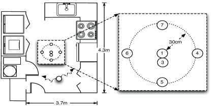
Figure 2: Floorplan for our indoor test environment and layout of sensor motes. Node 1 is the stationary base station (Alice) and Node 2 (Bob) is fixed to a robotic platform that moves randomly throughout the test environment. The remaining five nodes are passive eavesdropper nodes (Eve) that simply record all observed frames and their observed RSSI values.

We conducted two separate data collection experiments in a basic indoor residential environment. In each experiment, we placed the stationary base station (Alice) in the middle of the environment with five eavesdropper nodes placed around the base station as shown in Figure 2. The mobile node (Bob) was mounted to a purpose-built robotic platform that was programmed to move throughout the environment in a random pattern for the duration of the experiment at a rate of approximately 14 cm/sec while avoiding obstacles. The robot would move forward for a period of time selected uniformly at random from between 5 and 15 seconds. At the end of the randomly selected travel time, the robot would turn at an angle selected uniformly at random from between -75 to 75 degrees indicating a left or right turn, respectively. If the robot detected an obstacle via its front-mounted bump sensors or ultrasonic sensor before the time expired, the robot would similarly choose a new direction and travel time at random. The travel time and turn angles were selected primarily based on the small size of the test environment.

Each sensor mote can store up to 25,000 channel measurements and so, with a 1300ms delay between PING frames, each experiment represents approximately nine hours of continuous movement over a total distance traveled of around 4 kilometers per experiment. The data for each node from both experiments were concatenated together resulting in slightly less than 50,000 samples for each node after accounting for lost or dropped frames. Note that the number of samples we collected is for the purpose of our security analysis; an actual key can be computed much faster. See Section IV-D for more details on the number of samples required for key extraction.

IV-C Security Analysis of Our Key Extraction Protocol

Each experimental dataset was downsampled by six samples in order to simulate a greater idle time between PING frames and ensure that a channel sample $X_{i}$ is correlated only with $X_{i-1},X_{i+1}$, the reasoning will be explained in Section IV-E. After downsampling, we still have around 8100 samples in the experiment. We took 8000 samples and divided them into 100-sample slices, each slice representing a single key experiment.

Learning the conditional min-entropy: First, we estimate the average case min-entropy of Alice’s channel measurements given a single adversary’s view using the methodology proposed in Section III by incorporating the data from the key experiments. In our setup, there are 5 adversarial nodes and we calculated the entropy for each one separately. All our measurements were calculated for 32 distinct signal levels. Moreover, to make our adversarial model stronger, we simply ignored for both Alice and Bob all samples that were not also observed by Eve. By doing so, we ensure that we could obtain security without relying on frames missed by the eavesdropper.

For every experiment of 100 samples, we first compute the maximum conditional probability of the observed sequence by using the Viterbi algorithm and forward algorithm as explained in Section III; After getting the conditional min-entropy for the 80 key experiments, we average them to approximate the average case min-entropy due to the assumption that the conditional min-entropies on specific observations are stably distributed (experimental justification will appear in Figure 7).

Since $X_{i}$, the random variable representing Alice’s $i$-th sample, follows the same distribution for all $i$ (will be justified in Section IV-E), we get the initial state distribution $\pi$ by counting throughout all channel samples. We prepare the state transition probability matrix $A$ by estimating entry $a_{ij}$ by $\frac{n_{j}}{n_{i}}$, where $n_{j}$ is the number of measurements equal to $s_{i}$ such that the next measurement equals $s_{j}$, and $n_{i}$ is the number of measurements equal to $s_{i}$. Similarly, we approximate entry $b_{j}(k)$ for the observation probability distribution by $\frac{m_{k}}{m_{j}}$ where $m_{j}$ is the number of Alice’s measurements equal to $s_{j}$, and $m_{k}$ is the number of Eve’s observations equal to $o_{k}$ while the corresponding measurements of Alice is $s_{j}$. This is reasonable since the observation probability does not change (the independent observation assumption).

With all these parameters, we next apply the Viterbi algorithm and forward algorithm to compute the maximum conditional probability $\mathop{\max}_{x_{1},\ldots,x_{100}}\Pr[X_{1}=x_{1},\ldots,X_{100}=x_{100}|y_{1},\ldots,y_{100}],$ for every experiment, where $y_{1},\ldots,y_{100}$ are Eve’s measurements for a 100-sample slice. We then apply minus logarithm to those probabilities, and average them to get our final approximation for the average case min-entropy contained in 100 samples of Alice. Comparisons for the five nodes are shown in the sixth column of Table I.

Node	$M$	$n$	$N$	$\bar{d}$	H	$R_{e}$	$R$
3	80	100	800	4.42	88.40	0.55%	11.05%
4	80	100	800	4.29	99.82	0.54%	12.48%
5	80	100	800	4.36	98.89	0.55%	12.36%
6	80	100	800	4.28	93.07	0.54%	11.63%
7	80	100	800	4.35	94.08	0.54%	11.76%

TABLE I: Comparison of conditional min-entropy for the 5 eavesdropping nodes. $M$: # of experiments, $n$: # of channel samples in each experiment, $N=|\rho_{A}|$: the length of bit string after bit quantization, $\bar{d}$: the average # of word errors, $H$: the average case min-entropy, $R_{e}=d/|\rho_{A}|$: average error rate, and $R$: average entropy rate. The node IDs are as shown in Figure 2.

Accounting for Entropy Loss: With a reasonable amount of entropy contained in Alice’s channel measurements, conditioned on adversary’s view, we now proceed to calculate the entropy loss for each step, and subtract those losses to get the final result about security of the key.

First, for the bit quantization step, the way we defined the embedding $\tau$, it is a one-to-one map so, obviously, there is no entropy loss during this step. Thus, $\widetilde{\textbf{H}}_{\infty}(\rho_{A}|\textbf{Y})=\widetilde{\textbf{H}}_{\infty}(\textbf{X}|\textbf{Y}).$

Next we consider the entropy loss in the information reconciliation step. Suppose an $(n,k)$ binary code is used to construct the syndrome based secure sketch $u$ described in the protocol shown in Fig 1, a total of $|u|=n-k$ bits are transmitted during the information reconciliation step. Thus,

$$\widetilde{\textbf{H}}_{\infty}(\rho_{A}|\textbf{Y},u)=\widetilde{\textbf{H}}_{\infty}(\mathbf{X}|\textbf{Y},u)\geq\widetilde{\textbf{H}}_{\infty}(\textbf{X}|\textbf{Y})-|u|.$$

Finally, according to lemma 1, if $\widetilde{\textbf{H}}_{\infty}(\rho_{A}|\textbf{Y},u)\geq s\geq l+2\log\frac{1}{\epsilon_{u}}$, we can apply a $(t,s,l,\epsilon_{u})$ strong average case extractor to extract a key of length $l$ with distribution $\epsilon_{u}$ close to the uniform distribution over $\{0,1\}^{l}$.

Summarizing above, we derive a sufficient condition for extracting a secure key. Note that as long as the error rate is not too high, and there is a non-zero entropy left after the phase of information reconciliation, it is always possible to amplify the entropy by collecting more samples before the bit quantization step, and leaves room for privacy amplification.

IV-D Instantiation of Our Protocol

In this section, we will instantiate our general protocol for physical layer key extraction with concrete parameters from the experimental data.

We first study how conditional entropy grows in a block of samples with different size. By taking 10 samples as a unit, we slice the 8000 samples into 40 pieces, each representing an individual experiment with 200 samples. We then calculate conditional min-entropy (of 10 samples, 20 samples, and so forth until 200 samples) using our methodology by averaging among these 40 experiments. In this way we get the plot of the average conditional min-entropy with standard deviation of the 40 values as shown in Figure 3. We use the method of least squares to get an approximation of the average case min-entropy as a linear function of the number of samples and obtain the following equation: $g(x)=\frac{985}{1000}x+\frac{1467}{1000},$ i.e., there is $g(x)$ bits average case min-entropy in every $x$ samples.

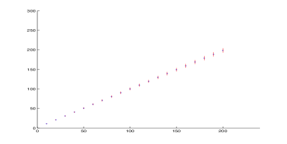
Figure 3: Linear growth of conditional min-entropy for node4, x-axis is the number of samples in the sequence, y-axis is the value of conditional min-entropy, the (blue) points are average of conditional min-entropy in 40 experiments, the (red) lines start from mean-standard deviation and extend to mean+standard deviation.

Similarly, we study the distribution of word (8-bit block) errors. We first divide the bitstrings $\rho_{A},\rho_{B}$ in 8-bit blocks, and count the number of different blocks between $\rho_{A},\rho_{B}$. The result is presented in Figure 4. In this way we obtain an approximation of the average word error $e$: $e(x)=\frac{43}{1000}x+\frac{48}{1000},$ which means there are $e(x)$ word errors on average in $x$-sample experiment.

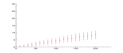
Figure 4: Distribution of errors, x-axis is the number of samples, y-axis is the number of errors, the (blue) points are average among 40 experiments, the (red) lines start from mean-standard deviation to mean+standard deviation

Our results experimentally show the linear growth of conditional min-entropy and that of errors. We can now provide an explicit instantiation of our protocol.

Theorem 1

Suppose $n$ is number of samples in our protocol. Using a Reed-Solomon code over $F_{2^{8}}$ for the sketch, when $n\geq\max\{12.54\lambda+6.27l-3.24,2326c-1\}$, we can successfully implement a $(l,e^{-c},2^{-\lambda})$ key generation system.

Proof:

Given the estimated conditional entropy rate as $g(n)=\frac{985}{1000}n+\frac{1467}{1000}$, and error rate as $e(n)=\frac{43}{1000}n+\frac{48}{1000}$, we choose a RS code over $F_{2^{8}}$ which can correct up to $\frac{6}{5}e(n)$ errors (slice the bitstring into proper sized blocks if needed). Thus, the entropy loss of applying the code would be $8\cdot 2\cdot\frac{6}{5}e$, the entropy loss of applying extractor is $2\lambda$, and similar to the analysis at the end of section IV-C, we immediately get: if $159.4n+549.4>1000l+2000\lambda$, we will have a $l$-bits key with $2^{-\lambda}$ distance to $U_{l}$. For correctness, from the Chernoff bound, the probability of having $\frac{6}{5}e(n)$ errors is $e^{\frac{-e(n)}{100}}$, we can easily derive another condition. ∎

To put the above into perspective, if we set $\epsilon_{c}=e^{-1},\epsilon_{u}=2^{-80}$, we can do the following: first we make around 1800 measurements, then use a 8-bit unary encoding on the absolute value. (We take only 5-bit precision for the RSSI value.) Finally, we employ a (255,229)-RS code for secure sketch and apply 2-universal hash functions [39] as randomness extractor and harvest a 128-bit key. Note that the success rate of the exchange is at least $1-\frac{1}{e}$ and is detectable by the parties hence in case of failure the extraction is repeated.

IV-E Justification of Channel Assumptions

We now show that all channel assumptions stated in Section III hold based on the analysis of the experimental data collected in the test environment described in Section IV-B.

Stationary Memoryless Markov Process Assumption: We split assumption 1 to three sub-assumptions. Let us begin with the assumption that every channel measurement $X_{i}$ depends only on the previous measurement $X_{i-1}$ for all $i$. As mentioned in our description of our test platform, we used an artificial delay of 1300ms between ping frames in order to induce independence between channel samples greater than one sample apart. To evaluate this assumption of independence we performed the following analysis. We selected some $i\in[1+m,n]$ uniformly at random, where $n$ is the number of samples in a node’s measurements, and $m=500$. We then created a $(m+1)$-length row vector as $\{X_{i},X_{i-1},\ldots,X_{i-m}\}$, where $X_{i-m}$ is the $(i-m)$-th sample from a node’s channel measurements. This was repeated 10,000 times, concatenating each of the 10,000 row vectors together to create a $10000\times(m+1)$ matrix $A$.

The Pearson’s linear correlation coefficients of the resulting column vectors in $A$ were then computed to find the correlation of $X_{i}$ with $X_{i-k}$ for each $k\in[1,500]$. From the correlation analysis of our experimental data, we found that there exists a statistically correlation between samples $X_{i}$ and $X_{i-k}$ at a significance level of $\alpha=0.05$ for values of $k$ up to $6$. Since we want to ensure that $X_{i}$ and $X_{i-k}$ are independent for $k>1$ for our channel assumptions to hold, we further downsample the collected data by a factor of six in order to induce this level of independence (i.e., ensuring at least 7800ms between samples). The remainder of our experimental analysis is performed on this downsampled data.

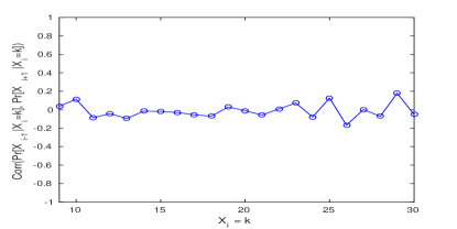
Figure 5: Correlation between $\Pr[X_{i-1}|X_{i}=k]$ and $\Pr[X_{i+1}|X_{i}=k]$ for channel sample values $k\in[9,29]$.

We further show that for all channel samples $X_{i}=k$, where $k$ is a 5-bit RSSI value, that $\Pr[X_{i-1}|X_{i}=k]$ and $\Pr[X_{i+1}|X_{i}=k]$ are uncorrelated. For every value of $k\in[0,32]$, we derive the distributions $\Pr[X_{i-1}|X_{i}=k]$ and $\Pr[X_{i+1}|X_{i}=k]$ and again compute the Pearson’s linear correlation coefficient between the two vectors. In our experimental dataset, value of $k<9$ and $k>29$ were infrequent and so we were unable to compute statistically significant correlation coefficients for those values of $k$. The remaining values of $k\in[9,29]$, however, constitute approximately 95% of our channel samples. The correlation coefficients between the two distributions for each value of $k\in[9,29]$ are shown in Figure 5. Our results show that $\Pr[X_{i-1}|X_{i}=k]$ and $\Pr[X_{i+1}|X_{i}=k]$ are uncorrelated for values of $k$ that have a sufficient number of samples (approximately 50 or more).

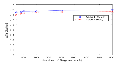
Figure 6: Computed WSS quotient values for varying segment sizes.

Finally, we consider the assumption that the Markov process transition probability is stationary. That is, we want to show that: $\Pr[X_{i}=x_{1}|X_{i-1}=x_{0}]=\Pr[X_{j}=x_{1}|X_{j-1}=x_{0}],$ holds for any $i$ and $j$ with $i\neq j$. For this test, we use the wide-sense stationarity (WSS) quotient [41] to evaluate whether the first and second moments of our experimental dataset. We computed the WSS quotient for multiple segment sizes ($S$) and provide the results in Figure 6. Our results show a high level of stationarity for the first and second moments of our sample data across all tested values of $S$. We also performed a series of K-S tests with similar results.

Stationary Observation Probability Assumption: Next, we consider our assumption 2 that the channel sample observation probability is stationary. Specifically, we want to show that $\Pr[Y_{i}=y|X_{i}=x]=\Pr[Y_{j}=y|X_{j}=x]$ holds true for any two sample indices $i$ and $j$ with $i\neq j$, where $x$ and $y$ indicate concrete RSSI values observed by Alice and Eve, respectively. We can easily find the correlation between $Y_{i}$ and $X_{i}$ for $k\in[-500,500]$ for each Eve node using the same approach based on computing the linear Pearson’s correlation coefficient that we described above for evaluating the first assumption. The results were averaged across all five eavesdropper nodes. We found that an eavesdropper measurement $Y_{i}$ was statistically independent from some sample $X_{j}$ collected by Alice for $i\neq j$ at a significance level of $\alpha=0.05$.

We use a technique similar to those above to evaluate whether $\Pr[Y_{i}|X_{i}]=\Pr[Y_{j}|X_{j}]$ for any two sample indices $i$ and $j$ with $i\neq j$). We first partition the set of sample indices $I=\{1,2,\ldots,N\}$ into two equal-sized random subsets $I^{\prime}_{1}$ and $I^{\prime}_{2}$ such that $|I^{\prime}_{1}|=|I^{\prime}_{2}|=\lfloor n/2\rfloor$. Eve’s channel measurement set $Y$ was similarly partitioned into two subsets $Y^{\prime}_{1}$ and $Y^{\prime}_{2}$, such that $Y^{\prime}_{1}$ contains the measurements in $Y$ corresponding to the channel sample indices in $I^{\prime}_{1}$ and $Y^{\prime}_{2}$ contains the measurements in $Y$ corresponding to the channel sample indices in $I^{\prime}_{2}$. Alice’s channel measurements were partitioned into two subsets $X^{\prime}_{1}$ and $X^{\prime}_{2}$ in the same manner. We then compute the joint distributions between $X^{\prime}_{1}$ and $Y^{\prime}_{1}$, as well as between $X^{\prime}_{2}$ and $Y^{\prime}_{2}$. For each RSSI value $x\in[-24,0]$ (the range of possible RSSI values in our experimental platform), we use a two-sample K-S test to determine whether the two distributions $\Pr[Y^{\prime}_{1}|X^{\prime}_{1}=x]$ and $\Pr[Y^{\prime}_{2}|X^{\prime}_{2}=x]$ are identical. This process was repeated a total of 10,000 times for each of the five eavesdropper sets $Y$ (i.e., a total of 50,000 trials). Out of the 50,000 trials, we accepted the null hypothesis that the two distributions were identical 100% of the time with a significance level of $\alpha=0.05$ and so we conclude that the assumption $\Pr[Y_{i}|X_{i}]=\Pr[Y_{j}|X_{j}]$ holds true when $i\neq j$.

Independent Observation Assumption: This states that the dependency that potentially exists between the adversary’s measurements comes strictly from the existing dependency of the corresponding measurements of Alice and not any other source. Note that from assumption 2, each $Y_{i}$ follows a distribution that depends only on the value of $X_{i}$ and this dependency does not change over time. This suggests that there exists a probabilistic function $F$ over $X_{i}$ which can simulate the observations of Eve, i.e., $Y_{i}=F(X_{i})$. In such case we can prove the independent observation assumption:

$$\Pr[Y_{1}=y_{1},\ldots,Y_{n}=y_{n}|x_{1},\ldots,x_{n}]$$

$$= \Pr[F(X_{1})=y_{1},\ldots,F(X_{n})=y_{n}|x_{1},\ldots,x_{n}]$$

$$= \Pr[F(x_{1})=y_{1},\ldots,F(x_{n})=y_{n}]$$

$$= \prod_{i=1}^{n}\Pr[F(x_{i})=y_{i}]=\prod_{i=1}^{n}\Pr[F(X_{i})=y_{i}|X_{i}=x_{i}]$$

$$= \prod_{i=1}^{n}\Pr[Y_{i}=y_{i}|X_{i}=x_{i}]$$

Stable Conditional Min-Entropy Assumption: The intuition for assumption 4 is that even though at some location, some observations may have better advantage to predict the original measurement, the sequence would be long enough, and thus when averaging across the whole sequence, the advantage will diminish. To experimentally justify this assumption, we calculate the min-entropy of the sequence received by node1 conditioned on node4’s observation in each experiment (represented by each 100-sample block). We observe that it is stably distributed as shown in Figure 7.

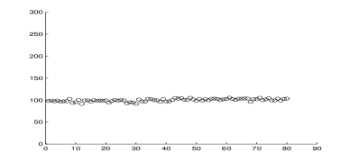
Figure 7: Distribution of conditional min-entropy in node4, x-axis is the index of experiment, y-axis is the value of conditional min-entropy, 300 is the maximum entropy contained in the 100 samples

V Conclusions and Future work

In this paper we presented a framework for a rigorous experimental security analysis that guarantees a reasonable level of security about the agreed key extracted from physical quantities, and we show an application of the framework to key extraction from wireless signals with concrete parameters based on our experimental data. Our novel methodology relies on HMM model and the estimation of conditional min-entropy through a dynamic programming approach that relies on the Viterbi and forward algorithms. Our work lays a comprehensive methodology for arguing experimentally the security of physical-layer key extraction against a passive eavesdropper nodes and can be applied to a number of other similar protocols in a similar way as we demonstrated here. At a very high level, our methodology entails the following basic steps, (i) employ a falsifiable channel abstraction, equipped with an efficient conditional entropy approximation algorithm and the execution of experiments that estimate the conditional min-entropy using the algorithm (ii) justify experimentally the channel abstraction, (iii) account for the entropy loss incurred due to quantization and information reconciliation.

While the above is a step forward in the security analysis of physical-layer key extraction there is still limited evidence for the security of these protocols in general settings; multitude of open questions remain and our methodology can be extended in a number of directions: (i) increase the size of the HMM or even substitute the HMM with more general Bayesian networks to improve the accuracy of the estimation of conditional min-entropy and potentially decrease the time needed for key generation. (ii) consider the case of active adversaries and develop protocols with adversarial interference detection for which conditional min entropy can still be effectively estimated. (iii) consider observations from multiple eavesdropper nodes simultaneously.

References

- [1] G. Brassard and L. Salvail, “Secret-key reconciliation by public discussion,” in EUROCRYPT, 1994, pp. 410–423.
- [2] C. H. Bennett, G. Brassard, and J.-M. Robert, “Privacy amplification by public discussion,” SIAM J. Comput., vol. 17, no. 2, pp. 210–229, 1988.
- [3] A. D. Wyner, “The wiretap channel,” Bell system technical journal, vol. 54, pp. 1355–1387, 1975.
- [4] U. M. Maurer, “Secret key agreement by public discussion from common information,” IEEE Trans on Information Theory, vol. 39, no. 3, pp. 733–742, 1993.
- [5] R. Ahlswede and I. Csiszar, “Common randomness in information theory and cryptography. i. secret sharing,” IEEE Trans on Information Theory, vol. 39, no. 4, pp. 1121–1132, 1993.
- [6] C. H. Bennett and G. Brassard, “Quantum cryptography: Public key distribution and coin tossing,” in ICASSP, 1984, pp. 175–179.
- [7] M. Bloch, J. Barros, M. R. D. Rodrigues, and S. W. McLaughlin., “Wireless information-theoretic security,” IEEE Transactions on Information Theory, vol. 54, no. 6, pp. 2515–2534, 2008.
- [8] J. Barros and M. R. D. Rodrigues, “On the secrecy capacity of wireless channels,” in Proceedings of the IEEE ISIT, 2006.
- [9] A. Khisti, S. N. Diggavi, and G. W. Wornell, “Secret-key generation using correlated sources and channels,” IEEE. Trans. on Inf. Forensics and Security, 2011.
- [10] P.K.Gopala, L.Lai, and H.ElGamal, “On the secrecy capacity of fading channels,” IEEE Trans on Inf. Theory, vol. 54, pp. 4687–4698, 2008.
- [11] L.Lai, Y.Liang, and H. Poor, “A unified framework for key agreement over wireless fading channels,” in IEEE ISIT, 2009.
- [12] M. Clark, “Robust wireless channel based secret key extraction,” in MilComm’12, pp. 1–6.
- [13] J. E. Hershey, A. A. Hassan, and R. Yarlagadda, “Unconventional cryptographic keying variable management,” IEEE Transactions on Communications, vol. 43, no. 1, pp. 3–6, 1995.
- [14] A. A. Hassan, W. E. Stark, J. E. Hershey, and S. Chennakeshu, “Cryptographic key agreement for mobile radio,” Digital Signal Processing, vol. 6, no. 4, pp. 207–212, 1996.
- [15] M.A.Tope and J.C.McEachen, “Unconditionally secure communications over fading channels,” in MilComm, 2001, pp. 54–58.
- [16] S. Jana, S. N. Premnath, M. Clark, S. K. Kasera, N. Patwari, and S. V. Krishnamurthy, “On the effectiveness of secret key extraction from wireless signal strength in real environments,” in MOBICOM, 2009, pp. 321–332.
- [17] B. Azimi-Sadjadi, A. Kiayias, A. Mercado, and B. Yener, “Robust key generation from signal envelopes in wireless networks,” in ACM CCS, 2007, pp. 401–410.
- [18] N. Patwari, J. Croft, S. Jana, and S. K. Kasera, “High-rate uncorrelated bit extraction for shared secret key generation from channel measurements,” IEEE Trans. Mob. Comput., vol. 9, no. 1, pp. 17–30, 2010.
- [19] C. Ye, S. Mathur, A. Reznik, Y. Shah, W. Trappe, and N. B. Mandayam, “Information-theoretically secret key generation for fading wireless channels,” IEEE Trans on Information Forensics and Security, vol. 5, no. 2, pp. 240–254, 2010.
- [20] X. Li and E.P.Ratazzi, “Mimo transmissions with information-theoretic secrecy for secret key agreement in wireless networks,” in MilComm’05.
- [21] R. Wilson, D. Tse, and R. A. Scholtz, “Channel identification: Secret sharing using reciprocity in ultrawideband channels,” IEEE Trans on Information Forensics and Security, vol. 2, no. 3-1, pp. 364–375, 2007.
- [22] T. Aono, K. Higuchi, T. Ohira, B. Komiyama, and H. Sasaoka, “Wireless secret key generation exploiting reactance-domain scalar response of multipath fading channels,” Antennas and Propagation, IEEE Transactions on, vol. 53, no. 11, pp. 3776 – 3784, nov. 2005.
- [23] S. Mathur, W. Trappe, N. B. Mandayam, C. Ye, and A. Reznik, “Radio-telepathy: extracting a secret key from an unauthenticated wireless channel,” in MOBICOM, 2008, pp. 128–139.
- [24] Q. Wang, H. Su, K. Ren, and K. Kim, “Fast and scalable secret key generation exploiting channel phase randomness in wireless networks,” in INFOCOM, 2011, pp. 1422–1430.
- [25] Y. Wei, K. Zeng, and P. Mohapatra, “Adaptive wireless channel probing for shared key generation,” in INFOCOM, 2011, pp. 2165–2173.
- [26] M. Edman, A. Kiayias, and B. Yener, “On passive inference attacks against physical-layer key extraction,” in EUROSEC ’11, 2011.
- [27] N. Döttling, D. E. Lazich, J. Müller-Quade, and A. S. de Almeida, “Vulnerabilities of wireless key exchange based on channel reciprocity,” in WISA, 2010, pp. 206–220.
- [28] G. Valiant and P. Valiant, “Estimating the unseen: an n/log(n)-sample estimator for entropy and support size, shown optimal via new clts,” in STOC, 2011, pp. 685–694.
- [29] A. J. Goldsmith and P. Varaiya, “Capacity, mutual information, and coding for finite-state markov channels,” IEEE Transactions on Information Theory, vol. 42, no. 3, pp. 868–886, 1996.
- [30] K. Salamatian and S. Vaton, “Hidden markov modeling for network communication channels,” in SIGMETRICS ’01, 2001, pp. 92–101.
- [31] A.J.Viterbi, “Error bounds for convolutional codes and an asymptotically optimal decoding algorithm,” IEEE Transactions on Information Theory, vol. 13, pp. 260–269, 1967.
- [32] L.E.Baum and J.A.Eagon, “An inequality with applications to statistical estimation for probabilistic functions of markov processes and to a model for ecology,” Bulletin of the American Mathematical Sociaty, vol. 73, pp. 360–363, 1967.
- [33] A. Gupta, R. Krauthgamer, and J. R. Lee, “Bounded geometries, fractals, and low-distortion embeddings,” ser. FOCS ’03, 2003, pp. 534–543.
- [34] Y. Dodis, L. Reyzin, and A. Smith, “Fuzzy extractors: How to generate strong keys from biometrics and other noisy data,” in EUROCRYPT, 2004, pp. 523–540.
- [35] N. Nisan and D. Zuckerman, “Randomness is linear in space,” J. Comput. Syst. Sci., vol. 52, no. 1, pp. 43–52, 1996.
- [36] S. Eberz, M. Strohmeier, M. Wilhelm, and I. Martinovic, “A practical man-in-the-middle attack on signal-based key generation protocols,” in ESORICS, 2012, pp. 235–252.
- [37] M. Zafer, D. Agrawal, and M. Srivatsa, “Limitations of generating a secret key using wireless fading under active adversary,” IEEE/ACM Trans. Netw., vol. 20, no. 5, pp. 1440–1451, 2012.
- [38] R. Ostrovsky and Y. Rabani, “Low distortion embeddings for edit distance,” in In Proceedings of the Symposium on Theory of Computing, 2005, pp. 218–224.
- [39] L. Carter and M. N. Wegman, “Universal classes of hash functions,” J. Comput. Syst. Sci., vol. 18, no. 2, pp. 143–154, 1979.
- [40] L. R. Rabiner, “A tutorial on hidden markov models and selected applications in speech recognition,” in Proceedings of the IEEE, 1989, pp. 257–286.
- [41] O. Sheluhin, S. Smolskiy, and A. Osin, Self-similar Processes in Telecommunications, 2007.