Quench Dynamics in a Model with Tuneable Integrability Breaking
Abstract
We consider quantum quenches in an integrable quantum chain with tuneable-integrability-breaking interactions. In the case where these interactions are weak, we demonstrate that at intermediate times after the quench local observables relax to a prethermalized regime, which can be described by a density matrix that can be viewed as a deformation of a generalized Gibbs ensemble. We present explicit expressions for the approximately conserved charges characterizing this ensemble. We do not find evidence for a crossover from the prethermalized to a thermalized regime on the time scales accessible to us. Increasing the integrability-breaking interactions leads to a behavior that is compatible with eventual thermalization.
pacs:
02.30.Ik,03.75.Kk,05.70.LnI Introduction
Important advances in manipulating cold atomic gases have allowed recent experiments BlochNature02 ; WeissNature06 ; SchmiedmayerNature07 ; BlochNatPhys12 ; KuhrNature12 ; SchmiedmayerScience12 to realize essentially unitary time evolution for extended periods of time. Stimulated by such experiments, there has been immense theoretical effort (see, e.g., Ref. PSSV_RMP11, for a recent review) to understand fundamental questions about the nonequilibrium dynamics of quantum systems: Do observables in a subsystem relax to stationary values? If so, can expectation values be reproduced with a thermal density matrix? What governs how and to which values observables relax?
It is generally accepted that conservation laws and dimensionality play important roles in the time evolution of isolated quantum systems. This is highlighted by the ground-breaking experiments of Kinoshita, Wenger and Weiss WeissNature06 . There, it was found that a three-dimensional condensate of 87Rb atoms driven out of equilibrium rapidly relaxed to a thermal state (“thermalized”), whilst a condensate constrained to move in a single spatial dimension relaxed slowly to a nonthermal ensemble. It is thought that the presence of additional (approximate) conservation laws in the one-dimensional case lies at the heart of this difference.
Theoretical investigations on translationally invariant models have established two central paradigms for the late time behavior after a quantum quench: (1) subsystems thermalize and are then described by a Gibbs ensemble (GE) nonint ; (2) subsystems do not thermalize, but at late times after the quench are described by Generalized Gibbs ensembles (GGE). There is substantial evidence BS_PRL08 ; CrEi ; CEF_PRL11 ; FE_PRB13 ; CC_JStatMech07 ; IC_PRA09 ; BKL_PRL10 ; FM_NJPhys10 ; EEF:12 ; Pozsgay_JStatMech11 ; CCR_PRL11 ; CIC_PRE11 ; CK_PRL12 ; CE_PRL13 ; MC_NJPhys12 ; FE:13b ; Pozsgay:13a ; Mussardo_arXiv13 ; CSC:13b ; KCC:13a ; KSCCI that the latter case applies quite generally to quenches in quantum integrable models, as suggested in a seminal paper by Rigol et al.GGE
The dichotomy in the dependence of stationary behavior after a quench on integrability then poses an intriguing question: what happens if integrability is weakly broken? Does the system thermalize, and if so, how fast does it relax? Might there be an intermediate time scale still governed by the physics of integrability?
Early numerical studies Manmana0709 suggested that even with an integrability breaking term the system does not thermalize on the accessible time scales and system sizes. Studies using analytical methodsMoeckel080910 for and numerical methods in the dynamical mean field limitKollarPRB11 () showed that on intermediate time scales the system approaches a nonthermal quasistationary state (a prethermalization plateau). At later times the system is expected to thermalize.BKL_PRL10 ; thermalize Prethermalization plateaus have also been observed in a nonintegrable quantum Ising chain with long-range interactions.MMGS_arXiv13 It has been suggested recently,BCK_arXiv13 that the time scale for integrability breaking (leaving the prethermalization plateau) is not necessarily related to the strength of the integrability breaking term. Experimental evidence for the prethermalization plateau in systems of bosonic cold atoms was reported in Refs. SchmiedmayerNJP11, ; SchmiedmayerScience12, ; SchmiedmayerEPJ13, . In spite of the aforementioned works exhibiting prethermalization plateaus in specific models, a general understanding of if, when and how such plateaus emerge when integrability is broken remains open. Similarly, a precise characterization of such plateaus in terms of statistical ensembles has not been achieved.
In this work we study the effects of integrability breaking interactions on the dynamics following a quantum quench. Our setup allows us to compare integrable quantum quenches to quenches where an additional integrability-breaking interaction is added to the post-quench Hamiltonian. By combining analytical calculations with time-dependent density matrix renormalization group (t-DMRG) results we demonstrate the existence of a prethermalization plateau in the sense that local observables relax to nonthermal values at intermediate times. We characterize this prethermalization plateau in terms of a novel statistical description, that we call the “deformed GGE”.
This paper is organized as follows. In Sec. II we introduce the model under study. In section III we consider integrable quenches and compare the observed stationary behavior to thermal and generalized Gibbs ensembles. The continuous unitary transformation technique is introduced and used to study a weakly nonintegrable quench of the model in Sec. IV. In Sec. V we establish the existence of the prethermalized regime and describe the approximately stationary behavior in this regime by constructing a “deformed GGE”. The dynamics in the presence of strong integrability-breaking interactions is studied numerically in Sec. VI. Sec. VII contains a summary and discussion of our main results. Technical details underpinning our analysis are consigned to several appendices.
II The Model
We consider the following Hamiltonian of spinless fermions with dimerization and density-density interactions
| (1) | |||||
with periodic boundary conditions. Here and we restrict our attention to the parameter regime , and . We work at half-filling throughout, i.e. the total number of fermions is . When showing results for the time evolution of observables we measure time in units of throughout. An important characteristic of is that fermion number is conserved by virtue of the symmetry
| (2) |
The presence of the symmetry is a crucial feature of our model: on the one hand it leads to dramatic simplifications in our analytical calculations, while at the same time it enables us to access very late times in our t-DMRG computations (as compared to existing studies of other nonintegrable one dimensional models).
We note that the Hamiltonian (1) is equivalent to a spin-1/2 Heisenberg XXZ chain with dimerized XX term as can be shown by means of a Jordan-Wigner transformation. The model with finite has previously been studied in order to investigate the effect of interactions on the equilibrium dimerization of the chain.SpinlessHubPeierls1 ; SpinlessHubPeierls2 Density matrix renormalization group calculations suggest that for large values of the interaction parameter , the Peierls transition to a dimerized ground state is suppressed.SpinlessHubPeierls2
There are several limits, in which exact results on the equilibrium phase diagram of are available. Firstly, in the absence of interactions () and for any value of the dimerization parameter we obtain a model of a noninteracting Peierls insulator. Secondly, for vanishing dimerization and a Jordan-Wigner transformation maps the model to the spin-1/2 Heisenberg XXZ chain. Finally, in the regime of small and , the low-energy limit of the model is given by the integrable sine-Gordon model.SGM
II.1 Peierls insulator
The special case describes a Peierls insulator and can be solved by means of a Bogoliubov transformation
| (3) |
Here are fermion annihilation operators fulfilling
| (4) |
The coefficients are chosen as
| (5) |
where
| (6) | |||||
| (7) |
The “” and “” bands are separated by an energy gap of . Finally, is a shorthand notation for the momentum sum
| (8) |
In terms of the Bogoliubov fermions the Peierls Hamiltonian is diagonal:
| (9) |
II.2 Integrability-breaking interactions
Adding interactions to the Peierls Hamiltonian leads to a theory that is not integrable. An exception is the low-energy limit for , which is described by a quantum sine-Gordon model.SGM In the following we will be interested in the regime , which is far away from this limit. It is useful to express the density-density interaction in in terms of the Bogoliubov fermions diagonalizing
| (10) | |||||
Here we have defined
| (11) | |||||
| (12) |
III Integrable Quantum Quenches
We first consider a quantum quench of the dimerization parameter in the limit of vanishing interactions . The system is initially prepared in the ground state of , and at time the dimerization is suddenly quenched from to . At times the system evolves unitarily with the new Hamiltonian .
The diagonal form of our initial Hamiltonian is
| (13) |
and describes two bands of noninteracting fermions. The ground state is obtained by completely filling the “” band; i.e.,
| (14) |
where is the fermion vacuum defined by , , . At times the system is in the state
| (15) |
The new Hamiltonian is diagonalized by the Bogoliubov transformation (3)
| (16) |
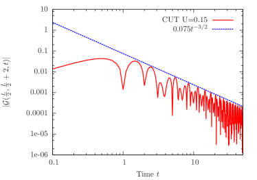
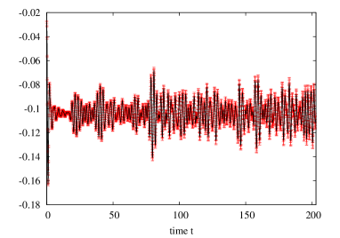
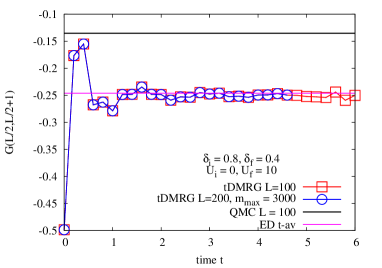
and by virtue of (3) the Bogoliubov fermions , are linearly related to , . Using this relation it is a straightforward exercise to obtain an explicit expression for the time evolution of the fermion Green’s function (see Fig. 1)
| (17) | |||||
where
| (18) |
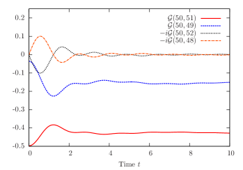
The late-time behavior can be determined by a stationary phase approximation, which gives
| (19) |
III.1 Generalized Gibbs ensemble (GGE)
The stationary state of the dimerization quench is described by a GGE.GGE We now briefly review the construction of the GGE following Refs. BS_PRL08, ; CEF_PRL11, ; FE_PRB13, . In the thermodynamic limit the system after the quench possesses an infinite number of local conservation laws (, )
| (20) |
An explicit construction of these conservation laws is presented in Appendix A. Given these conserved quantities we defined a density matrix
| (21) |
where ensures normalization.normalization The Lagrange multipliers are fixed by the requirements that the expectation values of the conserved quantities are the same in the initial state and in the GGE
| (22) |
We then bipartition the system into a segment B of contiguous sites and its complement and form the reduced density matrix
| (23) |
On the other hand the reduced density matrix of segment B after our quantum quench is simply
| (24) |
At late times after the quench it can be shown by using free fermion techniques (see, e.g., Ref. CEF_PRL11, ) that
| (25) |
An alternative GGE ; BS_PRL08 ; IC_PRA09 but equivalent FE_PRB13 construction of the GGE is based on the mode occupation numbers
| (26) |
By construction these commute with and among themselves, and we can express the density matrix in the form
| (27) |
The Lagrange multipliers are fixed by the conditions
| (28) |
which are solved by
| (29) |
Here the functions are defined in (18).
III.2 GGE vs. thermal expectation values
In the following it will be important to quantify the difference between the GGE constructed above and a Gibbs ensemble (GE)
| (30) |
constructed by requiring that the average thermal energy density is equal to the energy density in the initial state
| (31) |
Using the fact that the fermions diagonalizing and are linearly related by
| (32) |
we can rewrite (31) in the form
| (33) |
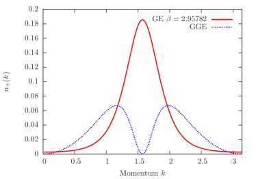
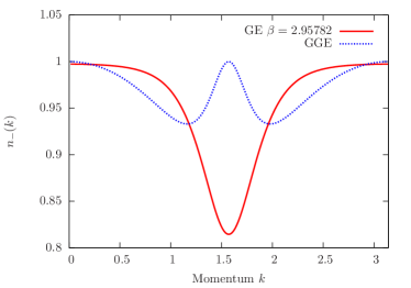
III.2.1 Mode occupation numbers
In order to exhibit the difference between Gibbs and generalized Gibbs ensembles it is useful to consider the mode occupation numbers, which are given by
| (34) |
III.2.2 Green’s function
As has been emphasized in Ref. CEF_PRL11, , as we are dealing with the nonequilibrium dynamics of an isolated quantum system, we should focus on the expectation values of local (in space) operators, as descriptions in terms of statistical ensembles most naturally apply to them (see also FE_PRB13 ; sirker13 ). We therefore consider the fermionic Green’s function in position space, and furthermore focus on its short-distance properties. The Green’s functions in the GGE and thermal ensembles are
| (35) |
where the mode occupation numbers are given by (34).
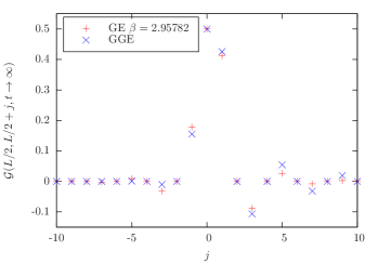
In Fig. 4 we show a comparison between the results for the fermion Green’s function calculated in the appropriate Gibbs and generalized Gibbs ensembles. We observe that in contrast to the mode occupation numbers, the difference between the short-distance behavior of the Green’s function in the two ensembles is fairly small.
IV Quenching to a weakly interacting model
We now modify our quantum quench as follows. We still start out our system in the ground state of the pure Peierls Hamiltonian given by Eq. (14), but we now quench to , where we consider to be small compared to . Our main interest is to quantify how a non-zero value of modifies the dynamics after the quench.
To tackle the quench problem in the nonintegrable weakly interacting model we employ the continuous unitary transformation (CUT) technique CUT ; KehreinBook which has been applied extensively to nonequilibrium problems (see, for example, Refs. CUT_NonEq, ; Moeckel080910, ). We provide a brief overview of the CUT technique for out-of-equilibrium many-body systems and proceed to calculate the time-dependent Green’s function and the four-point function.
IV.1 Time evolution of observables by CUT
For a nonintegrable interacting model it is no longer possible to calculate the time evolution induced by the Hamiltonian (1) exactly. We use the CUT technique to obtain a perturbative expansion in of the time-evolved observables.
The central idea of the CUT method is to construct a sequence of infinitesimal unitary transformations, chosen such that the Hamiltonian becomes successively more energy-diagonal. A family of unitarily equivalent Hamiltonians characterized by the parameter can be constructed from the solutions of the differential equation
| (36) |
where is the anti-Hermitian generator of the unitary transformation. Wegner CUT showed that the Hamiltonian in the final basis is energy diagonal if , where is the quadratic part of the Hamiltonian and is the remainder. In practice (36) is used by expanding all operators in power series in an appropriate small parameter, which in our case will be the interaction strength .
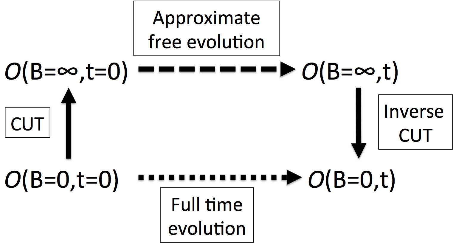
Following the transformation with an appropriate choice of generator, the Hamiltonian is energy diagonal (but not integrable). To perform the time evolution we must introduce an additional approximation: We normal order the interaction term with respect to the initial state and neglect the normal-ordered quartic (and higher order) terms
where the time evolution operator depends only on the quadratic Hamiltonian whose single particle energies have contributions. By construction this approximation introduces a maximal time scale, on which we expect our calculations to be accurate by virtue of the smallness of . Estimating this time scale within the CUT formalism is difficult, as it requires a reliable treatment of the neglected energy diagonal interaction terms. For this reason we extensively compare our CUT results to t-DMRG computations (see Sec. IV.5). Importantly, we can perform our CUT calculations for very large systems of hundreds of sites, for which we have verified that finite-size effects do not play a role on time scales less then the revival time (the results shown below are for times less than the revival time). The procedure for calculating the approximate time evolution of observables is shown schematically in Fig. 5.
IV.2 The canonical generator and flow equations for the Hamiltonian
We start by constructing the “canonical generator” of the unitary transformation KehreinBook given by
| (37) |
The flow-dependent operators are defined by
| (38) | |||||
| (39) | |||||
where the parameters in the Hamiltonian have been promoted to functions of the flow parameter and where the dots indicate terms sextic and higher in creation and annihilation operators. The canonical generator is given by
| (40) | |||||
where
By inserting the canonical generator (40) and the flow Hamiltonian
| (41) |
into the flow equation (36) and integrating the resulting differential equations, we find the flow-dependent single particle energies and interaction vertices
| (42) | |||||
| (43) |
Setting we obtain the Hamiltonian in the energy-diagonal basis
| (44) |
where indeed the interaction vertices conserve energy
| (45) |
We note that to leading order in the single particle energies remain unchanged by the unitary transformation. Having found the energy-diagonal form of the Hamiltonian to leading order we now consider the unitary transformation induced by the canonical generator (40) on the Green’s function.
IV.3 Green’s function
Our main objective is to determine the fermion Green’s function on the time-evolved initial state
| (46) |
Using the expression for the original fermions in terms of the Bogoliubov fermions , we see that
| (47) | |||||
where are defined in Eq. (5) and . Hence the basic objects we need to calculate are expectation values of . This is done by following the procedure set out in Fig. 5. The flow equations
| (48) |
are easily constructed to order and integrating them gives
| (49) |
where we have defined
| (50) |
IV.3.1 Approximate time evolution
In the next step of the procedure sketched in Fig. 5 we consider the time evolution induced by the Hamiltonian (44). We approximate the time evolution operator by
| (51) |
where the Hamiltonian has been replaced by the free fermion Hamiltonian
with single particle energies
| (52) |
The additional term is given by
where is defined in Eq. (45). The expectation values taken in the initial state are given by
| (54) | ||||
where functions are defined by Eq. (18). The correction to the single-particle energies arises from normal ordering the interaction term with respect to the initial state . The normal ordering prescription for the quartic term is given by
| (55) | |||||
The normal-ordered quartic interaction term on the right hand side of (55) has been neglected for the time evolution in Eq. (51). Following this approximation, the time evolution of fermion operators results only in additional phase factors
| (56) |
Using (56) in (49) provides an explicit expression for the time-evolved operators . In the final step shown in Fig. 5 we reverse the CUT. Integrating back to the initial basis , and then taking the expectation value with respect to the initial state we obtain
| (57) | |||||
Here the order piece is
| (58) |
where we have defined
| (59) |
IV.4 CUT results for the Green’s function
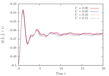
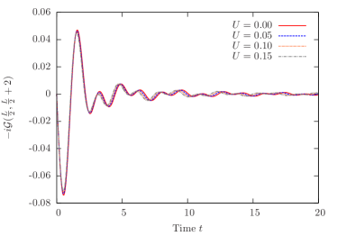
We first compare the CUT results to the exactly solvable case. Figures 6 and 7 show the nearest-neighbour and next-nearest-neighbour Green’s functions for the quench for several values of . With increasing the periodicity of the oscillations and the asymptotic value of the nearest neighbour Green’s function are continuously deformed away from the non-interacting result. The next-nearest-neighbour Green’s function is an imaginary quantity that decays asymptotically to zero for both the non-interacting and CUT result.
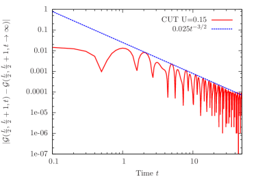
In Figs. 8 and 9 we show the fermion Green’s function for separations for the quench and for the chain. In both cases the long-time decay of the CUT result is compatible with the non-interacting power-law decay. This is a consequence of the fact that the CUT result (60) has the same general -dependence as the non-interacting case (17).
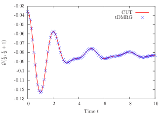
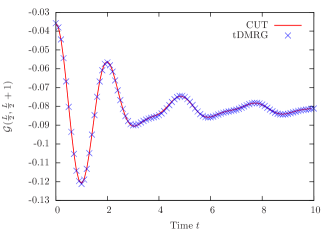
IV.5 Accuracy of the CUT approach: comparison to time-dependent density matrix renormalization group at small
In order to assess the accuracy of the CUT approach we have carried out extensive comparisons to numerical results obtained by the time-dependent density matrix renormalization group (t-DMRG) algorithm. As is customary in density matrix renormalization group studies, we impose open boundary conditions. We have carried out computations for systems up to lattice sites, but for the puposes of comparing to our CUT results we choose a system size of . Up to density matrix states were kept in the course of the time evolution, and a discarded weight of was targetted. In order to assess the accuracy of the results at later times, we carried out comparisons to results obtained with a target discarded weight of , and in addition compared to simulations using different time steps of or , respectively. Some details are presented in Appendix B. As shown there, the difference between the results at the end of the time evolution is or smaller for sites, which means t-DMRG errors are negligible in our comparison to the CUT results.
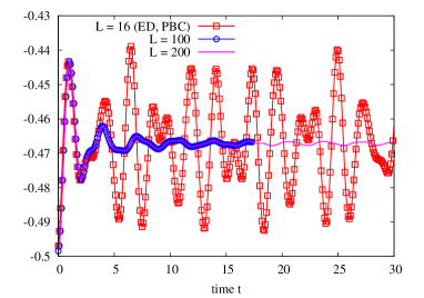
The revival time for measurements in the center of a finite chain of noninteracting particles is , where is the system size and is the maximal velocity. In the small- regime of interest here we can obtain a good estimate of by calculating it in the limit. The estimate can be improved by searching for features associated with revivals at times close to the free fermion estimate. By comparing data with different systems sizes , we have verified that finite-size effects are negligible in the t-DMRG data for times less than the revival time . Finally, we carry out a comparison between CUT and t-DMRG results only for times sufficiently smaller than . We note that as far as the t-DMRG computations are concerned, we have been able to reach times for system size . Whilst for short enough times the error in the observable can be estimated as , at longer times, even if the discarded weight is kept constant, the accumulation of errors in the course of the sweeps needs to be taken into account. Therefore, for the situations in which times are discussed, a more detailed error analysis is necessary, which is presented in Appendix B.
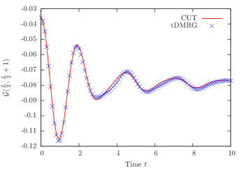
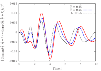
In Figs. 10–12 we show a comparison of the CUT and t-DMRG results for the time-dependence of the nearest-neighbour Green’s function for the length chain. We quench the dimerization parameter and the interaction strength , respectively. There is good, quantitative agreement between the CUT and t-DMRG results provided is small. The remaining discrepancies have their origin in the order corrections to the CUT results as is shown in Fig. 13, where we plot the rescaled difference between the t-DMRG data and the CUT result for three values of . The oscillatory nature of these differences can be explained as a ”beat frequency” arising from subtracting two oscillatory data sets where the frequencies don’t match exactly.
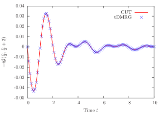
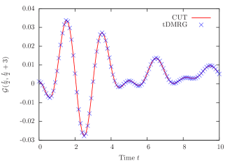
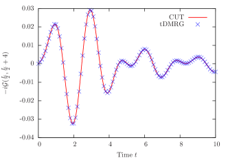
Figures 14–16 show that the good agreement between CUTs and t-DMRG is not limited to the nearest-neighbour Green’s function by comparing results for with for the case of .
IV.6 CUT results for the four-point function
The procedure which we have outlined above for the single-particle Green’s function can be generalized to -point functions. The next non-vanishing correlation function is the four point function
| (61) |
where are defined in Eq. (5) and
| (62) |
Going to the basis by applying the CUT and then time evolving with (51), we obtain
| (63) | |||||
where and are defined in Eq. (59). Taking the expectation value of Eq. (63) on the initial state using Wick’s theorem and substituting in to Eq. (61) yields the real-space four-point function.
V Prethermalized Regime
The combination of CUT and t-DMRG results establish that at intermediate times the fermion Green’s function after a quench decays in a power-law fashion with approximate exponent to a stationary value; i.e.,
| (64) |
It is very instructive to compare this to the result (19) for the quench . By virtue of the perturbative nature of the CUT approach, and its excellent agreement with t-DMRG for small and the time scales relevant to the present discussion, we obtain the following relation between the asymptotic values of the Green’s function for the two quenches
| (65) |
We will now show that cannot be described by a thermal ensemble, which implies that the stationary regime observed by t-DMRG is in fact a prethermalization plateau.
-
1.
For the quench the observed plateau corresponds to the true stationary state and is characterized by a GGE, i.e.
(66) -
2.
As we showed in Sec. III.2, the GGE expectation values for the Green’s function are generally different from the thermal expectation values at the appropriate effective inverse temperature characterizing the quench
(67) -
3.
If the stationary state after the quench was described by a thermal distribution, its effective inverse temperature would be determined by
(68) On the other hand, given that Wick’s theorem holds in the state , we conclude that
(69) Hence
(70) - 4.
- 5.
V.1 Characterization of the prethermalized regime through approximate conservation laws
In the previous section we have shown that the CUT result cannot produce an effective thermal Gibbs ensemble in the long time limit. Given that the CUT results for the Green’s function are in excellent agreement with t-DMRG data at intermediate times, this establishes the existence of a “prethermalized stationary regime”. An obvious question is then how to characterize the statistical ensemble describing the corresponding plateau values of local observables.
V.1.1 Approximate conservation laws
In our CUT analysis of the nonequilibrium dynamics the generator of time evolution was taken to be
| (73) |
Clearly the mode occupation number operators commute with , and hence constitute conservation laws (to first order in ) within our CUT approach. Their pre-images under the CUT, accurate to order , are simply
| (74) | |||||
By construction these operators approximately commute with one another
| (75) |
However, the commutator with the Hamiltonian is in fact
| (76) |
i.e. the charges (74) are not (approximately) conserved on an operator level, but only their expectation values with respect to are (approximately) time independent. This is a fundamental difference to the proposal put forward in Ref. KollarPRB11, for describing prethermalization plateaus. The charges have a very transparent physical meaning: they are the number operators for approximately conserved “quasiparticles”, and the quartic terms describe the leading contribution to the dressing of the non-interacting fermions.
V.1.2 Approximate description by a “deformed GGE”
It is natural to attempt a description of the prethermalized regime in terms of a statistical ensemble of the form
| (77) |
Here the Lagrange multipliers are fixed by the requirements
| (78) |
The left-hand side of (78) is most easily evaluated in the basis, where it becomes
| (79) |
The right-hand side of (78) is equal to
| (80) |
Equating (80) with (79) and using (54) we obtain an explicit expression for the Lagrange multipliers . The fermion Green’s function evaluated with respect to the density matrix (77) is
| (81) | |||||
We wish to show that this is equal to the infinite-time limit of the CUT result up to order corrections, i.e.
| (82) |
The trace in (81) is most easily evaluated in the basis
| (83) | |||||
Substituting (83) into (81) we obtain an expression that indeed agrees with the infinite-time limit of (60) in the thermodynamic limit . This establishes (82). Hence the Green’s function (for fixed in the thermodynamic limit) on the prethermalization plateau is described by the GGE (77) with deformed charges (74). This observation is consistent with a description of local observables on the prethermalization plateau in terms of a deformed GGE. On the other hand there are non-local operators, being a simple example, which in fact do not relax at intermediate times and are therefore not described by the ensemble (without time-averaging).
V.1.3 “Deformed GGE” description of the four-point function
The preceding section shows that the value of the Green’s function on the prethermalization plateau is given by the deformed GGE . We now show that the deformed GGE also reproduces the expectation value of the CUT result for the four-point function (61). We wish to calculate
| (84) |
with given in (77). As in the previous section, this trace is most easily performed in the basis
| (85) | |||||
where . The GGE expectation values are easily calculated using Wick’s theorem and (78). Retaining only terms up to and substituting the result back into (84), we obtain the deformed GGE value for the four-point function on the prethermalization plateau.
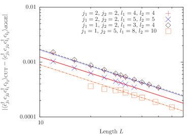
In Fig. 17 we plot the difference between the deformed GGE result obtained in this way and the stationary value of the CUT result (found by projecting on to the stationary terms of Eq. (61)) for a number of system sizes and separations. In all cases the difference between the CUT and deformed GGE results scales as and vanishes in the thermodynamic limit . This confirms that the stationary value of the CUT four-point function is reproduced by the deformed GGE (77). This is a rather non-trivial check of our proposal that prethermalization plateaus can be described in terms of a deformed GGE.
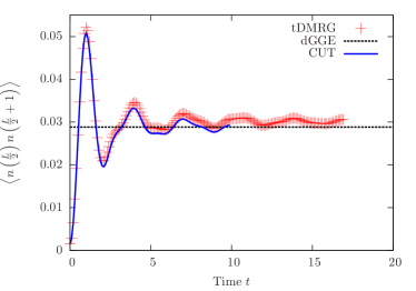
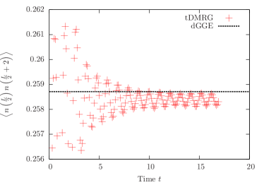
In Figs. 18 and 19 we present comparisons between t-DMRG results and predictions of the deformed GGE for nearest-neighbor and next-nearest-neighbor density-density correlation functions (84) for the quench and . Taking into account that is not particularly small, the observed agreement between the two results is quite satisfactory. This supports our assertion that the deformed GGE provides a good description of higher-order correlation functions on the prethermalization plateau. We see similarly good agreement for all separations (up to sites) that we explicitly checked. The deformed GGE predictions and the CUT result of Fig. 18 are calculated for system sizes rather than , because the computational cost of carrying out the momentum sums in the expression for the four-point function (61) increases very rapidly with system size.
VI t-DMRG results for larger values of and absence of thermalization on accessible times scale
In this section we turn to numerical results obtained for quenches to final Hamiltonians with both weak and strong interactions, i.e., when . As can be seen, in all cases the time evolution seems to reach a plateau and remains - on the accessible time scales - on this plateau. This is observed for quenches starting from a non-interacting initial state as well as when .
VI.1 Extent of prethermalization plateaus
The first issue we want to address is the time scale over which we observe prethermalization plateaus. In Figs. 10–12 and 14-16 results are shown only up to in order to avoid revivals. The prethermalization plateau for persists to much later times of at least , as can be seen in Fig. 20, where we present data for . On the accessible time scales there is no sign that the system starts to deviate from the plateau at late times.
VI.2 Time averages
A standard method for extracting stationary values of observables from finite systems is to consider time-averaged quantities, e.g.
| (86) |
For the system shown in Fig. 20 the average over long times is in good agreement with the plateau value for the and data. One question that can be asked is whether time averages may reveal signs of the system deviating from the prethermalization plateau. In order to investigate this issue, we have carried out t-DMRG simulations for a system up to very late times . The results are shown in Fig. 21.
Time averages of the t-DMRG data do not reveal any signs of deviations from the plateau value at late times.
VI.3 The role of interactions in the pre-quench and post-quench Hamiltonians
In this section we present results for a variety of interaction strengths in the post-quench Hamiltonian, as well as for quenches from the ground state at a finite value of the interactions. We provide two benchmarks for comparison:
VI.3.1 Gibbs Ensemble
One useful comparison is with the appropriate Gibbs ensemble describing a putative thermal ensemble at late times. We have computed these by quantum Monte Carlo (QMC) using the ALPS collaboration ALPS directed loop stochastic series expansion SSE code. Using the Jordan-Wigner transformation to map onto a spin model, the QMC calculations are performed in the grand canonical ensemble; the chemical potential and the effective temperature are fixed to ensure the correct energy and number densities (within the QMC error): these are given in Table 1 (see also Figs. 22–29).
| U | QMC | ||||
| Error | |||||
| 0.4 | -0.664373 | 3.0741 | 0.4 | -0.46358 | |
| 1 | -0.589142 | 2.6494 | 1 | -0.46247 | |
| 2 | -0.463757 | 2.0437 | 2 | -0.44347 | |
| 3 | -0.338371 | 1.5882 | 3 | -0.40153 | |
| 4 | -0.212986 | 1.2175 | 4 | -0.34284 | |
| 6 | 0.037784 | 0.7250 | 6 | -0.23885 | |
| 8 | 0.288550 | 0.4868 | 8 | -0.17441 | |
| 10 | 0.539324 | 0.3591 | 10 | -0.13514 |
In the QMC simulations of the chain we perform thermalization steps and perform measurements of the nearest-neighbour Green’s function after sweeps.
VI.3.2 Diagonal Ensemble
A second useful benchmark is provided by the diagonal ensemble. Given an initial state and a basis of energy eigenstates, the diagonal ensemble average of an observable is defined as
| (87) |
For finite systems this equals the long-time average (over many recurrences). We compute the diagonal ensemble for a system of sites by exact diagonalization (ED).
VI.3.3 Difference between diagonal and Gibbs averages
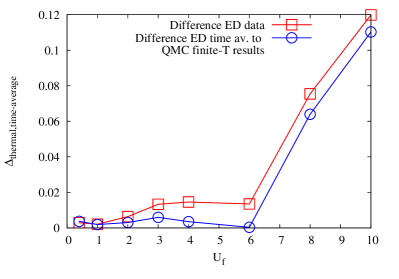
In Fig. 30 we show the difference between the expectations values of the nearest-neighbour Green’s function in the diagonal and Gibbs ensembles respectively for different values of . As the diagonal ensemble is available only for system size , we display the quantities
| (88) |
We see that for small values the two averages are close to one another, but for large they become very different.
VI.3.4 Results
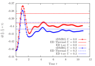
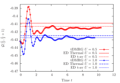
As can be seen from Figs. 22, 28 and 29, the nearest-neighbour Green’s function approaches plateaus values at late times, which are compatible with the diagonal ensemble (given that the latter was calculated for L=16 we expect there to be finite-size effects), but not the Gibbs ensemble.
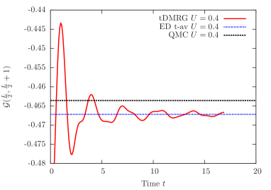
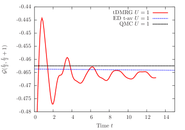
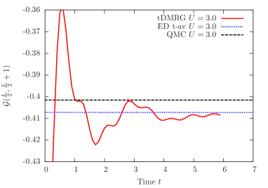
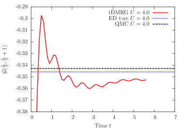
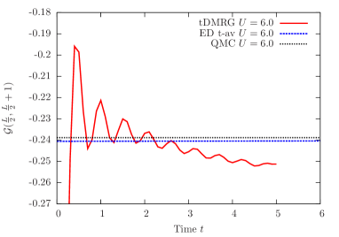
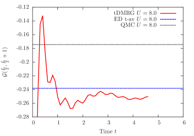
On the other hand, the plateau for intermediate values is compatible with a thermal ensemble on the accessible time scales. We propose the following explanation for these observations:
-
1.
The small- regime is described by a prethermalization plateau as discussed in section V. It can be understood in terms of a deformation of the generalized Gibbs ensemble characterizing the stationary state of the quench.
-
2.
The large- regime is also described by a prethermalization plateau, which now can be understood in terms of a deformation of the generalized Gibbs ensemble characterizing the stationary state of the quench. This corresponds to a quench to the Heisenberg XXZ chain in the massive regime. Given that our initial state has a short correlation length, GGE expectation values of local observables could be calculated by the method of Ref. FE:13b, . In order to test our interpretation, we have investigated the dependence of the plateau value on ( corresponding to an integrable quench in the XXZ chain).
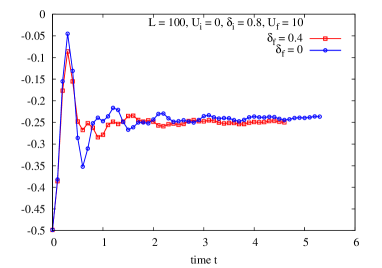
Figure 31: (Color online) Comparison of t-DMRG results for the time evolution of for systems with sites for quenches with initial to values of and or , respectively. As can be seen, the expectation value for both cases is very similar. In Fig. 31 we show a comparison between quenches to and or , respectively. The correlator clearly approaches a plateau, the value of which is only very weakly dependent on the integrability-breaking parameter , which supports our interpretation.
-
3.
In the intermediate- regime there is no prethermalization plateau, but the system relaxes slowly towards a Gibbs ensemble.
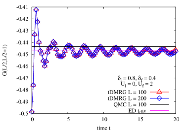
VI.3.5 Initial-state dependence
A final issue we would like to address is whether our findings are sensitive to our particular choices of initial state. In order to assess this question we have carried out t-DMRG computations for quenches starting in the ground state of strongly interacting Peierls insulators, i.e. Hamiltonians . Results for quenches of the form
| (89) |
with several values of are shown in Figs. 32 & 33. Here the expectation values of both the diagonal and Gibbs ensembles have been computed for site systems. Hence finite-size effects should be taken into account when making comparisons to the t-DMRG data.
The observed behavior is qualitatively very similar to that seen for quenches starting in non-interacting ground states. Observables relax to plateaus values that are incompatible with thermalization when is either small or large.
VII Conclusions
Using a combination of anaytical calculations based on the continuous unitary transform technique and time-dependent density matrix renormalization group computations we have established the existence of a robust prethermalization regime at intermediate times after a quantum quench to the weakly nonintegrable interacting Peierls insulator Hamiltonian (1). The combination of analytical and numerical techniques we use to analyze this plateau enables us to essentially eliminate finite-size effects. Our results thus represent true “bulk” physics, and in particular are free from revival effects. To the best of our knowledge, our work constitutes the first one dimensional example of a robust prethermalization plateau in a model with short-range interactions.
The CUT results allowed us to explicitly construct a “deformed generalized Gibbs ensemble”, which provides an approximate statistical description of the prethermalization plateau. The deformed GGE is constructed from charges cf Eq. (74), that form a mutually commuting set but do not commute with the Hamiltonian (44). As such, the deformed charges are not conserved at the operator level; only the expectation values with respect to the time-evolved state are approximately conserved. Our construction is therefore quite different from that of Ref. KollarPRB11, . We conjecture that the deformed GGE idea applies more widely to quantum quenches in one-dimensional models with weak integrability breaking. It would be interesting to test this conjecture for other examples.
We expect that at very late times the system will actually thermalize, but we are not able to access sufficiently long times scales with either the perturbative CUT approach or t-DMRG. A possible approach to describe the dynamics at very late times might be through a quantum Boltzmann equation (see, e.g., Refs. QuantumBoltz, ). This possibility is currently under investigation.
Acknowledgements
We thank A. Chandran, M. Fagotti, M. Kolodrubetz, M. Rigol and S. Sondhi for stimulating discussions. This work was supported by the EPSRC under Grants No. EP/I032487/1 (F.H.L.E and N.J.R) and No. EP/J014885/1 (F.H.L.E). S. K. and S. R. M. acknowledge support through SFB 1073 of the Deutsche Forschungsgemeinschaft (DFG).
Appendix A Local conservation laws for
To derive the local conservation laws for the non-interacting Hamiltonian we follow Appendix C of Ref. FE_PRB13, . Below we give the local conservation laws and summarize the salient points of the derivation.
The Hamiltonian can be written in the form
where are Majorana fermions defined by
and is a skew-symmetric block-circulant matrix of the form
| (94) |
where are matrices with and . We define the Fourier transform of the block matrices as
with .
For free fermions a complete set of local conservation laws can be given by fermion bilinears
where the matrices must satisfy
| (95) |
The problem of deriving local conservation laws has now become the problem of finding a set of mutually commuting matrices that also commutes with the Hamiltonian matrix . At first sight the complexity of the problem does not seem to have been reduced, but we can now utilize a useful property of the Hamiltonian matrix : the projectors onto eigenvectors of block circulant matrices are themselves block circulant matrices. This means one can consider that are block circulant:
| (100) |
Imposing Eqs. (95), we obtain the conditions (for all )
where is the Fourier transform of .
The construction of is straightforward as
where
So takes the form
where the functions , , and are chosen such that the Fourier transform satisfies .
The ambiguity in choice of functions leads to different representations of the conservation laws; following Ref. FE_PRB13, we make a particular choice that ensures there is a finite real-space range of the conservation laws: for . We consider the conservation laws associated with each of the terms in separately and Fourier transforming back to real space we find
where is a measure of the locality of the conservation laws and takes values to .
The local conservation laws are independent of the microscopic parameters of the theory; they arise from the and terms in . The remaining local conservation laws are dependent on the dimerization parameter . Energy conservation is also manifest in the set of local conservation laws with .
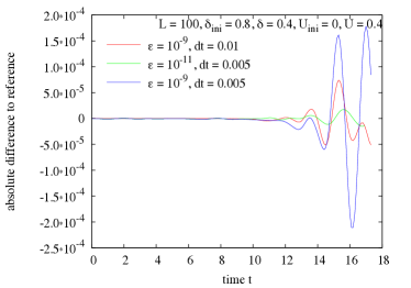
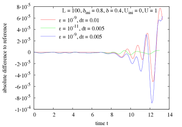
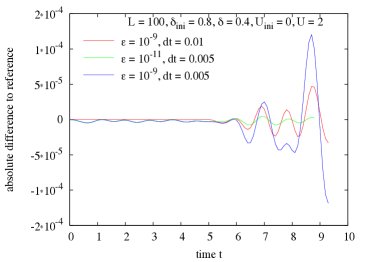
Appendix B Error estimate for the t-DMRG
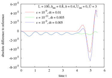
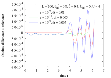
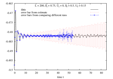
In this appendix, we estimate the error for the long time simulations. In principle, the error in a given observable can be estimated by the discarded weight , and due to the variational nature of the DMRG for ground state calculations, it is white2007 . At short times this provides a reasonable estimate for time-evolved quantities as well. On longer time scales a number of complications emerge. 1) Due to the entanglement growth, the discarded weight grows quickly in time.gobert2005 This can be addressed by adjusting the number of density matrix eigenstates, so that is smaller than a chosen threshold (in our case or for some simulations, respectively). 2) The error due to the Trotter decomposition becomes sizable. 3) Errors incurred in the sweeping procedure accumulate. In each DMRG step, the change of basis needed during the sweeps introduces an error as a result of the basis truncation. Hence, each sweep introduces an error for a system of size . This error is present at each time step. After a certain time , a simulation with a step size leads to an error . This error is in addition to the error in the observable due to the density matrix truncation discussed above. At short times the error due to the basis truncation dominates, but at later times other error sources can no longer be neglected. This can be seen by varying both the target discarded weight and the time step. In Fig. 34 we show the difference of runs with different parameters to a reference run with and . The error between the results with a target discarded weight of and is seen to be roughly two orders of magnitudes, as expected from the above estimate. The error bars shown in Figs. 21 and 35 are estimated on the basis of the above considerations. The error bars grow significantly towards the end of the time evolution, but still permit us to make qualitative statements. For the runs considered, this indicates that on the time scales treated the quasistationary state does not change, i.e., the prethermalization plateau is still present. Together with ED results obtained for small systems for times up to , this indicates that thermalization happens at much larger time scales (), if at all.
 |
 |
 |
 |
 |
References
- (1) M. Greiner, O. Mandel, T. W. Hänsch, and I. Bloch, Nature 419, 51 (2002).
- (2) T. Kinoshita, T. Wenger, D. S. Weiss, Nature 440, 900 (2006); http://jila.colorado.edu/USJAPAN /pdf/Kinoshita.pdf.
- (3) S. Hoerberth, I. Lesanovsky, B. Fischer, T. Schumm, and J. Schmiedmayer, Nature 449, 324 (2007).
- (4) S. Trotzky Y.-A. Chen, A. Flesch, I. P. McCulloch, U. Schöllwock, J. Eisert, and I. Bloch, Nature Physics 8, 325 (2012).
- (5) M. Cheneau, P. Barmettler, D. Poletti, M. Endres, P. Schauss, T. Fukuhara, C. Gross, I. Bloch, C. Kollath, and S. Kuhr, Nature 481, 484 (2012).
- (6) M. Gring, M. Kuhnert, T. Langen, T. Kitagawa, B. Rauer, M. Schreitl, I. Mazets, D. A. Smith, E. Demler, and J. Schmiedmayer, Science 337, 1318 (2012).
- (7) A. Polkovnikov, K. Sengupta, A. Silva, and M. Vengalattore, Rev. Mod. Phys. 83, 863 (2011).
- (8) J. M. Deutsch, Phys. Rev. A 43, 2046 (1991); M. Srednicki, Phys. Rev. E 50, 888 (1994); M. Rigol, V. Dunjko, and M. Olshanii, Nature 452, 854 (2008); E. Canovi, D. Rossini, R. Fazio, G. Santoro, and A. Silva, New J. Phys. 14, 095020 (2012).
- (9) T. Barthel and U. Schollwöck, Phys. Rev. Lett. 100, 100601 (2008).
- (10) M. Cramer, C.M. Dawson, J. Eisert, T.J. Osborne, Phys. Rev. Lett. 100, 030602 (2008); M. Cramer, J. Eisert, New J. Phys. 12, 055020 (2010).
- (11) P. Calabrese, F.H.L. Essler, and M. Fagotti, Phys. Rev. Lett. 106, 227203 (2011); J. Stat. Mech. P07016 (2012); J. Stat. Mech. P07022 (2012).
- (12) M. Fagotti and F.H.L. Essler, Phys. Rev. B 87, 245107 (2013).
- (13) P. Calabrese and J. Cardy, J. Stat. Mech. P06008 (2007).
- (14) A. Iucci and M. A. Cazalilla, Phys. Rev. A 80, 063619 (2009).
- (15) G. Biroli, C. Kollath, and A.M. Läuchli, Phys. Rev. Lett. 105, 250401 (2010).
- (16) D. Fioretto and G. Mussardo, New J. Phys. 12, 055015 (2010).
- (17) F.H.L. Essler, S. Evangelisti and M. Fagotti, Phys. Rev. Lett. 109, 247206 (2012);
- (18) B. Pozsgay, J. Stat. Mech. (2011) P01011.
- (19) A. C. Cassidy, C. W. Clark, and M. Rigol. Phys. Rev. Lett. 106, 140405 (2011).
- (20) M. A. Cazalilla, A. Iucci, and M.-C. Chung, Phys. Rev. E 85, 011133 (2012).
- (21) J.-S. Caux and R. M. Konik, Phys. Rev. Lett. 109, 175301 (2012).
- (22) J. Mossel and J.-S. Caux, New J. Phys. 14, 075006 (2012).
- (23) J.-S. Caux and F.H.L. Essler, Phys. Rev. Lett. 110, 257203 (2013).
- (24) M. Fagotti and F.H.L. Essler, J. Stat. Mech. Theor. Exp. (2013) P07012.
- (25) B. Pozsgay, J. Stat. Mech. Theor. Exp. P07003 (2013).
- (26) G. Mussardo, arXiv:1304.7599 (2013).
- (27) M. Collura, S. Sotiriadis and P. Calabrese, Phys. Rev. Lett. 110, 245301 (2013); J. Stat. Mech. (2013) P09025.
- (28) M. Kormos, M. Collura and P. Calabrese, Phys. Rev. A 89, 013609 (2014).
- (29) M. Kormos, A. Shashi, Y.-Z. Chou, J.-S. Caux and A. Imambekov, Phys. Rev. B 88, 205131 (2013).
- (30) M. Rigol, V. Dunjko, V. Yurovsky, and M. Olshanii, Phys. Rev. Lett. 98, 050405 (2007).
- (31) S. R. Manmana, S. Wessel, R. M. Noack, and A. Muramatsu, Phys. Rev. Lett. 98 210405 (2007); Phys. Rev. B 79, 155104 (2009); C. Kollath, A. M. Läuchli, and E. Altman; Phys. Rev. Lett. 98, 180601 (2007).
- (32) M. Moeckel and S. Kehrein, Phys. Rev. Lett. 100, 175702 (2008); Ann. Phys. 324, 2146 (2009); New J. Phys. 12, 055016 (2010).
- (33) M. Kollar, F. A. Wolf, and M. Eckstein, Phys. Rev. B 84, 054304 (2011).
- (34) M. Rigol, Phys. Rev. Lett. 103, 100403 (2009); M. Rigol, Phys. Rev. A 80, 053607 (2009); L. F. Santos and M. Rigol, Phys. Rev. E 81, 036206 (2010); L. F. Santos and M. Rigol, Phys. Rev. E 82, 031130 (2010).
- (35) M. Marcuzzi, J. Marino, A. Gambassi, and A. Silva, Phys. Rev. Lett. 111, 197203 (2013).
- (36) G. Brandino, J.-S. Caux, and R. M. Konik, arXiv:1301.0308 (2013).
- (37) T. Kitagawa, A. Imambekov, J. Schmiedmayer and E. Demler, New J. Phys. 13, 073018 (2011).
- (38) T. Langen, M. Gring, M. Kuhnert, B. Rauer, R. Geiger, D. A. Smith, I. E. Mazets, J. Schmiedmayer Eur. Phys. J. Special Topics 217, 43 (2013).
- (39) V. Y. Krivnov and A. A. Ovchinnikov, Zh. Eksp. Teor. Fiz, 90,709 (1986); Sov. Phys. JETP 63 414 (1986).
- (40) C. Schuster and U. Eckern, Eur. Phys. J. B 5, 395 (1998).
- (41) T. Nakano and H. Fukuyama, J. Phys. Soc. Jpn 50, 2489 (1981); F.H.L. Essler and R.M. Konik, in “From Fields to Strings: Circumnavigating Theoretical Physics”, ed. M. Shifman, A. Vainshtein, J. Wheater, World Scientific, Singapore (2005); cond-mat/0412421.
- (42) In practice we consider a very large system of size and take into account conserved quantities.
- (43) J. Sirker, N.P. Konstantinidis, F. Andraschko, N. Sedlmayr, arXiv:1303.3064.
- (44) F. Wegner, Ann. Physik (Leipzig) 3, 77 (1994); J. Phys. A 39 8221 (2006); S. D. Glazek and K. G. Wilson, Phys. Rev. D 48, 5863 (1993); Phys. Rev. D 49, 4214 (1994).
- (45) S. Kehrein, The Flow Equation Approach to Many-Particle Systems (Springer, 2006).
- (46) S. Kehrein, Phys. Rev. Lett. 95, 056602 (2005); A. Hackl and S. Kehrein, Phys. Rev. B 78, 092303 (2008).
- (47) B. Bauer et al. (ALPS collaboration), J. Stat. Mech. P05001 (2011).
- (48) A. W. Sandvik and J. Kurkijärvi, Phys. Rev. B 43, 5950 (1991); A. W. Sandvik, J. Phys. A 25, 3667 (1992).
- (49) L. P. Kadanoff and G. Baym, Quantum Statistical Mechanics (Benjamin, New York, 1962); J. Rammer and H. Smith, Rev. Mod. Phys. 58, 323 (1986); M.L.R. Fürst, C.B. Mendl and H. Spohn, Phys. Rev. E86, 031122 (2012); M. Tavora and A. Mitra, Phys. Rev. B, 88, 115144 (2013).
- (50) S.R. White and A.L. Chernyshev, Phys. Rev. Lett. 99, 127004 (2007).
- (51) D. Gobert, C. Kollath, U. Schollwöck, and G. Schütz, Phys. Rev. E 71, 036102 (2005).