PoS(LATTICE 2013)499
ADP-13-25/T845
DESY 13-221
Edinburgh
2013/33
LTH 994
Electromagnetic splitting of quark and pseudoscalar meson masses from dynamical
QCD QED
R. Horsleya, Y. Nakamurab, D. Pleiterc,
P.E.L. Rakowd, e, H. Stübenf,
R.D. Youngg and
J.M. Zanottig
a School of Physics and Astronomy, University of Edinburgh, Edinburgh
EH9 3JZ, United Kingdom
b RIKEN Advanced Institute for Computational Science, Kobe, Hyogo
650-0047, Japan
c JSC, Forschungszentrum Jülich, 52425 Jülich, Germany
d Theoretical Physics Division, Department of Mathematical Sciences,
University of Liverpool, Liverpool L69 3BX, United Kingdom
e Deutsches Elektronen-Synchrotron DESY, 22603 Hamburg, Germany
f RRZ, University of Hamburg, 20146 Hamburg, Germany
g CSSM, School of Chemistry and Physics, University of Adelaide,
Adelaide SA 5005, Australia
QCDSF Collaboration
Abstract:
Lattice QCD simulations are now reaching a precision where
electromagnetic corrections from QED become important. In
investigating the effects of breaking due
to quark mass differences within QCD, a group-theoretical analysis of
the mass dependence greatly helped us organize our results. We now do
the same with electromagnetic charge effects by extending the
calculations to dynamical flavor QCD + QED.
1 Introduction
One of the most profound open questions in particle physics is to
understand the pattern of flavor symmetry breaking and mixing, and the
origin of CP violation. In [1] we have outlined a
program to systematically investigate the pattern of flavor symmetry
breaking. The program has been successfully applied to meson and
baryon masses involving up (), down () and strange () quarks.
A distinctive feature of our simulations is the way we tune the light
and strange quark masses. We have our best theoretical understanding
when all three quark flavors have the same mass, because we can use
the full power of flavor . Starting from the
symmetric point, our strategy is to keep the singlet
quark mass fixed at its
physical value, while is varied. As we move from the symmetric point
(where the pion mass is )
to the physical point along the path ,
the quark becomes heavier, while the and quarks become
lighter. These two effects tend to cancel in any flavor singlet
quantity. To leading order, the cancellation is exact at the symmetric
point, and we
have found that it remains good down to the lightest points we have
simulated so far [1].
In order to compute physical observables to high precision, it is
important to include and control contributions from QED. Recent
lattice investigations of electromagnetic (EM) corrections to hadron
observables have been performed on pure QCD background
configurations [2], while a simulation with dynamical
photons, including meson-photon mixing effects, is still missing. In this
project we will extend our previous simulations of flavor QCD
with SLiNC fermions to a fully dynamical simulation of flavor
QCD + QED.
2 QCD + QED pseudoscalar meson mass formulae
In pure QCD [1] our strategy was
to start from a point with all three sea quark
masses equal, , and extrapolate towards the physical
point by keeping the average sea quark mass
constant. For this trajectory to reach the physical point we
start at a point , where with
equal to its physical value. That is
. We call this point the physical SU(3)
symmetric point. We denote the distance from by , . This forms a plane, as we have the constraint
. The bare quark masses are
defined by
(1)
where gives the quark mass at the physical SU(3) symmetric point,
and where vanishing of all quark masses along the line
determines . The quark masses
are subject to additive and multiplicative renormalization, while the
reference point gets multiplicatively renormalized
only [1].
In this presentation we shall concentrate on the pseudoscalar meson octet. The
expansion around , valid for the outer ring of the
pseudoscalar octet, was found to be [1]
(2)
for arbitrary quarks , with and being the LO and NLO expansion coefficients, respectively.
It is useful, in many respects, to vary valence and sea quark masses
independently. This is referred to as partial quenching (PQ). In this
case the sea quark masses remain constrained by ,
while the valence quark masses are
unconstrained. Defining , we obtain the
PQ mass formula
(3)
When , this result reduces to the previous
result (2). The coefficients that appear in the expansion
about the flavor symmetric point (2) and in the PQ case
(3) are the same. Hence this offers a computationally cheaper
way of obtaining them.
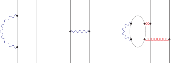
Figure 1: Examples of Feynman diagrams contributing to the
meson electromagnetic mass to order .
The symmetry of the electromagnetic current is similar to the symmetry
of the quark mass matrix. The simplifications that come from the
constraint in the mass case
are similar to the simplifications we get from the
identity . One difference between quark mass
and electromagnetic expansions is that in the mass
expansion we can have both odd and even powers of ,
whereas we are only allowed even powers of the quark charges. We can
therefore read off the leading QED corrections
from [1], dropping the linear terms and
changing masses to charges. For the outer mesons, and also for the
partially quenched mesons with all annihilation diagrams
turned off, we find
(4)
The coefficients in (4) can be matched up with
different classes of Feynman diagrams shown in Fig. 1. The
first diagram, with both ends of the photon attached to the
same valence quark, contributes to as well as . The second diagram, with the photon crossing between the
valence lines, only
contributes to and . The last
diagram, with the photon
being attached to the sea quarks, is an example of a diagram
contributing to and . It would
be missed out if the
electromagnetic field was quenched instead of dynamical.
Except for , and , all
coefficients can be determined by PQ simulations at our expansion
point. The term
can be absorbed into . The coefficients and
require simulations with unequal sea quark masses.
Many of the terms in (4) cancel in the combination
(5)
that will be important in our later discussions.
3 Lattice setup
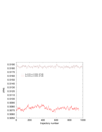
Figure 2: The average plaquette for and
on the lattice
for (bottom red line) and (top gray line) as a
function of trajectory number.
The action we are using is
(6)
Here is the tree-level Symanzik improved SU(3) gauge action,
and is the noncompact U(1) gauge action [3]
of the photon,
(7)
The fermion action for each flavor is
(8)
where is a single iterated mild stout
smeared link [1]. The clover coefficient
has been computed nonperturbatively [4]. The quark
charges are and (in units of ). We
presently neglect EM modifications to the clover term. This will leave
us with corrections of , which are presumably smaller than
the corrections from QCD.
Upon integrating out the Grassmann variables in the partition
function, and rewriting the resultant determinant using
pseudofermions, the effective action reads (generically)
(9)
where is the fermion matrix. We deal with the square root
of by rewriting it as a rational function
(10)
and employ the Rational Hybrid Monte Carlo (RHMC)
algorithm [5]. At the
symmetric point, , this reduces to
quark species. Then the Hybrid Monte Carlo (HMC) algorithm can be used
for the and
quarks, while the RHMC algorithm is used for the quark. Away from
the symmetric point we would not expect to run into a sign problem as
we will always keep .
4 Preliminary results and discussion
Our first dynamical QCD + QED simulation was done on the lattice at and . That is at the flavor symmetric point . We chose . In Fig. 2 we
compare the average plaquette with and without dynamical photons. The
difference is significant. Our strategy is to simulate
at an artificially large coupling , and
then interpolate between this point and pure QCD to the physical
coupling .
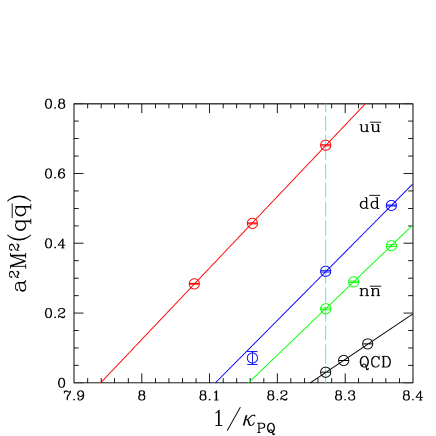
As a first application we have looked at the EM mass shifts of quark
and pseudoscalar meson masses. In Fig. 3 we show PQ masses
for , and a
fictitious electrically neutral quark , , as a
function of the PQ hopping parameter .
The first point to notice is that the mesons have become much heavier,
especially the . We attribute this mostly to a shift in
for the quarks, due to their electromagnetic self-interaction, which
amounts to an additive quark mass renormalization. We
would obviously expect this to be a bigger effect for the than for
the or quark, as observed. At the flavor symmetric point,
, we find
(11)
This is to be compared with the corresponding mass of pure QCD,
[1]. We estimate the
lattice spacing to be smaller than in pure QCD,
using the vector meson mass for determining the change in scale.
A reasonable definition of the additive quark mass renormalization for
each flavor is
(12)
where is the critical hopping parameter of QCD, and
the PQ critical hopping parameter can be read off
from Fig. 3. We find
(13)
This is to be compared with the quark mass of pure QCD at the flavor
symmetric point, . Note that , as expected.
Our present fits give
and , assuming a linear dependence on
. Both and come almost
entirely from the shifts in . From PCAC and the leading
flavor expansion we expect
that . Violations
of this relation cannot be present at leading order in the quark
mass. In our data the and terms
cancel, and the only term which contributes at the expansion point
is ,
(14)
corresponding to the middle diagram in Fig. 1. From
our fits we obtain .
In order to understand the sign of , we note that
opposite charges attract and like charges repel. As a result, we would
expect EM effects to raise the mass of, for example, the
() meson relative to the and
mesons. That is exactly what we find, which is mirrored in a positive
sign of . We should, however, be aware that this
result might be contaminated by QCD and heavy quark effects.
Figure 3: Partially quenched QCD + QED pseudoscalar meson masses
for , and against
. Also shown are the PQ masses from pure QCD, as
given in [6].
Besides the mass splittings of mesons and baryons, we are interested
in the masses of , and quarks. A point to make is that the
renormalization factors will now depend on both the QCD and the QED
coupling, and the quark will have a different renormalization
factor and anomalous dimension from the other two quarks. This means
that the ratio now depends on renormalization scheme and
scale. Likewise, isospin-violating mass splittings, such as ,
are scheme
independent, but the question of how much of the
splitting is due to the quark mass differences, and how much is due to
EM effects, becomes dependent on scheme and scale.
5 Outlook
In pure QCD we can impose perfect SU(3) symmetry by making all three
values equal. With QED present, there is no way to have
perfect SU(3) symmetry with physical charge ratios. A physically
reasonable definition is to look
for a line, where the neutral pseudoscalar masses ,
as well as the PQ flavor diagonal masses ,
, (with annihilation diagrams turned
off) and are equal. We are currently using PQ
calculations to locate this line. The line will have
.
This symmetric line will end at a point, where all neutral
pseudoscalar mesons are massless. We define this to be the chiral
point. It is the point, where all our quark masses are zero. In the
case of the and quarks this is the correct definition. Even
with QED present, we have a chiral SU(2) symmetry connecting and
quarks. So, if both quarks are massless, there will be a massless
Goldstone boson from the spontaneous symmetry breaking. Although the
neutral pseudoscalar mesons will be massless at the chiral point, the
charged mesons can have a mass from EM effects. Furthermore, the
charged axial vector currents are no longer conserved after QED is
added to the action. Hence, there is no Goldstone boson for the
charged pseudoscalar sector.
To summarize, our strategy is to compute hadron observables, both in
QCD (which we have done already) and in QCD + QED with , the
average sea quark mass, to be the same (or nearly the same) in both
simulations. This we achieve by simulating at points, where the
QCD + QED pseudoscalar mesons have (approximately) the same mass as in
the pure QCD simulation. To obtain statistically significant results,
the calculations are performed at a suitable value of . We then
may interpolate the numbers to , knowing the
results at .
Acknowledgement
This work has been supported in part by the EU under contract 227431
(HadronPhysics2) and contract 283286 (HadronPhysics3), and the
Australian Research Council by grants FT120100821 (RDY) and
FT100100005 (JMZ). The numerical simulations have been performed on
JUQUEEN at JSC (Jülich) and DIRAC 2 at EPCC (Edinbugh), as well as on
ICE at HLRN (Berlin and Hannover).
References
[1]
W. Bietenholz et al.,
Phys. Rev. D 84, 054509 (2011)
[arXiv:1102.5300 [hep-lat]].
[2]
T. Blum et al.,
Phys. Rev. D 82 (2010) 094508
[arXiv:1006.1311 [hep-lat]];
S. Aoki et al.,
Phys. Rev. D 86 (2012) 034507
[arXiv:1205.2961 [hep-lat]];
G. M. de Divitiis et al.,
Phys. Rev. D 87 (2013) 114505
[arXiv:1303.4896 [hep-lat]];
S. Borsanyi et al.,
arXiv:1306.2287 [hep-lat].
[3]
M. Göckeler et al.,
Nucl. Phys. B 334, 527 (1990);
M. Göckeler et al.,
Nucl. Phys. B 371 (1992) 713.
[4]
N. Cundy et al.,
Phys. Rev. D 79 (2009) 094507
[arXiv:0901.3302 [hep-lat]].
[5]
M. A. Clark and A. D. Kennedy,
Phys. Rev. Lett. 98 (2007) 051601
[hep-lat/0608015].
[6]
R. Horsley et al.,
Phys. Rev. D 85 (2012) 034506
[arXiv:1110.4971 [hep-lat]].