Incremental Discovery of Prominent Situational Facts

Abstract

We study the novel problem of finding new, prominent situational facts, which are emerging statements about objects that stand out within certain contexts. Many such facts are newsworthy—e.g., an athlete’s outstanding performance in a game, or a viral video’s impressive popularity. Effective and efficient identification of these facts assists journalists in reporting, one of the main goals of computational journalism. Technically, we consider an ever-growing table of objects with dimension and measure attributes. A situational fact is a “contextual” skyline tuple that stands out against historical tuples in a context, specified by a conjunctive constraint involving dimension attributes, when a set of measure attributes are compared. New tuples are constantly added to the table, reflecting events happening in the real world. Our goal is to discover constraint-measure pairs that qualify a new tuple as a contextual skyline tuple, and discover them quickly before the event becomes yesterday’s news. A brute-force approach requires exhaustive comparison with every tuple, under every constraint, and in every measure subspace. We design algorithms in response to these challenges using three corresponding ideas—tuple reduction, constraint pruning, and sharing computation across measure subspaces. We also adopt a simple prominence measure to rank the discovered facts when they are numerous. Experiments over two real datasets validate the effectiveness and efficiency of our techniques.

I Introduction

Computational journalism emerged recently as a young interdisciplinary field [6] that brings together experts in journalism, social sciences and computer science, and advances journalism by innovations in computational techniques. Database and data mining researchers have also started to push the frontiers of this field [7, 8, 11]. One of the goals in computational journalism is newsworthy fact discovery. Reporters always try hard to bring out attention-seizing factual statements backed by data, which may lead to news stories and investigation. While such statements take many different forms, we consider a common form exemplified by the following excerpts from real-world news media:

• “Paul George had 21 points, 11 rebounds and 5 assists to become the first Pacers player with a 20/10/5 (points/rebounds/assists) game against the Bulls since Detlef Schrempf in December 1992.” (http://espn.go.com/espn/elias?date=20130205)

• “The social world’s most viral photo ever generated 3.5 million likes, 170,000 comments and 460,000 shares by Wednesday afternoon.” (http://www.cnbc.com/id/49728455)

What is common in the above two statements is a prominent fact with regard to a context and several measures. In the first statement, the context includes the performance of Pacers players in games against the Bulls since December 1992 and the measures are points, rebounds, assists. By these measures, no performance in the context is better than the mentioned performance of Paul George. For the second statement, the measures are likes, comments, shares and the context includes all photos posted to Facebook. The story is that no photo in the context attracted more attention than the mentioned photo of President Barack Obama, by the three measures. In general, facts can be put in many contexts, such as photos posted in 2012, photos posted by political campaigns, and so on.

Similar facts can be stated on data from domains outside of sports and social media, including stock data, weather data, and criminal records. For example: 1) “Stock A becomes the first stock in history with price over $300 and market cap over $400 billion.” 2) “Today’s measures of wind speed and humidity are $x$ and $y$, respectively. City B has never encountered such high wind speed and humidity in March.” 3) “There were 35 DUI arrests and 20 collisions in city C yesterday, the first time in 2013.” Some of these facts are not only interesting to reporters but also useful to financial analysts, scientists, and citizens.

In technical terms, a fact considered in this paper is a contextual skyline object that stands out against other objects in a context with regard to a set of measures. Consider a table $R$ whose schema includes a set of measure attributes $\mathcal{M}$ and a set of dimension attributes $\mathcal{D}$. A context is a subset of $R$, resulting from a conjunctive constraint defined on a subset of the dimension attributes $D\subseteq\mathcal{D}$. A measure subspace is defined by a subset of the measure attributes $M\subseteq\mathcal{M}$. A tuple $t$ is a contextual skyline tuple if no other tuple in the context dominates $t$. A tuple $t^{\prime}$ dominates $t$ if $t^{\prime}$ is better than or equal to $t$ on every attribute in $M$ and better than $t$ on at least one of the attributes. Such is the standard notion of dominance relation adopted in skyline analysis [5].

We study how to find situational facts pertinent to new tuples in an ever-growing database, where the tuples capture real-world events. We propose algorithms that, whenever a new tuple $t$ enters an append-only table $R$, discover constraint-measure pairs that qualify $t$ as a contextual skyline tuple. Each such pair constitutes a situational fact pertinent to $t$’s arrival.

tuple id	player	day	month	season	team	opp_team	points	assists	rebounds
$t_{1}$	Bogues	11	Feb.	1991-92	Hornets	Hawks	4	12	5
$t_{2}$	Seikaly	13	Feb.	1991-92	Heat	Hawks	24	5	15
$t_{3}$	Sherman	7	Dec.	1993-94	Celtics	Nets	13	13	5
$t_{4}$	Wesley	4	Feb.	1994-95	Celtics	Nets	2	5	2
$t_{5}$	Wesley	5	Feb.	1994-95	Celtics	Timberwolves	3	5	3
$t_{6}$	Strickland	3	Jan.	1995-96	Blazers	Celtics	27	18	8
$t_{7}$	Wesley	25	Feb.	1995-96	Celtics	Nets	12	13	5

* Attribute opp_team is the short form of opposition team.

TABLE I: A Mini-world of Basketball Gamelogs

Example 1.

Consider the mini-world of basketball gamelogs $R$ in Table I, where $\mathcal{D}$={player, month, season, team, opp_team} and $\mathcal{M}$={points, assists, rebounds}. The existing tuples are $t_{1}$ to $t_{6}$ and the new tuple is $t_{7}$. If the context is the whole table (i.e., no constraint) and the measure subspace $M$=$\mathcal{M}$, $t_{7}$ is not a skyline tuple since it is dominated by $t_{3}$ and $t_{6}$. However, with regard to context $\sigma_{\textsf{\footnotesize month}=\textsl{\footnotesize Feb.}}(R)$ (corresponding to constraint month=Feb.) and the same measure subspace $M$, $t_{7}$ is in the skyline along with $t_{2}$. In yet another context $\sigma_{\textsf{\footnotesize team}=\textsl{\footnotesize Celtics}\wedge}$ ${}_{\textsf{\footnotesize opp\_team}=\textsl{\footnotesize Nets}}(R)$ under measure subspace $M$={assists, rebounds}, $t_{7}$ is in the skyline along with $t_{3}$. Tuple $t_{7}$ is also a contextual skyline tuple for other constraint-measure pairs, which we do not further enumerate.  

Discovering situational facts is challenging as timely discovery of such facts is expected. In finding news leads centered around situational facts, the value of a news piece diminishes rapidly after the event takes place. Consider NBA games again. Sports media need to identify and discuss sensational records quickly as they emerge; any delay makes fans less interested in the records and risks losing them to rival media. Timely identification of situational facts is also critical in areas beyond journalism. To make informed investment decisions, investors want to know facts related to stock trading as soon as possible. Facts discovered from weather data can assist scientists in identifying extreme weather conditions and help government and the public in coping with the weather.

Simple situational facts on a single measure and a complete table, e.g., the all-time NBA scoring record, can be conveniently detected by database triggers. However, general and complex facts involving multiple dimension and measure attributes are much harder to discover. Exhaustively using triggers leads to an exponential explosion of constraint-measure pairs to check for each new tuple. In reality, news media relies on instincts and experiences of domain experts on this endeavor. The experts, impressed by an event such as the outstanding performance of a player in a game, hypothesize a fact and manually craft a database query to check it. This is how Elias Sports Bureau tackles the task and provides sports records (such as the aforementioned one by Paul George) to many sports media [1]. With ever-growing data and limited human resources, such manual checking is time-consuming and error-prune. Its low efficiency not only leads to delayed and missing facts, but also ties up precious human expertise that could be otherwise devoted to more important journalistic activities.

The technical focus of this paper is thus on efficient automatic approach to discovering situational facts, i.e., finding constraint-measure pairs that qualify a new tuple $t$ as a contextual skyline tuple. A straightforward brute-force approach would compare $t$ with every historical tuple to determine if $t$ is dominated, repeatedly for every conjunctive constraint satisfied by $t$ under every possible measure subspace. The obvious low-efficiency of this approach has three culprits—exhaustive comparison with every tuple, under every constraint, and over every measure subspace. We thus design algorithms to counter these issues by three corresponding ideas, as follows:

1) Tuple reduction   Instead of comparing $t$ with every previous tuple, it is sufficient to only compare with current skyline tuples. This is based on the simple property that, if any tuple dominates $t$, then there must exist a skyline tuple that also dominates $t$. For example, in Table I, under constraint month=Feb. and the full measure space $\mathcal{M}$, the corresponding context contains $t_{1}$, $t_{2}$, $t_{4}$ and $t_{5}$, and the contextual skyline has two tuples—$t_{1}$ and $t_{2}$. When the new tuple $t_{7}$ comes, with regard to the same constraint-measure pair, it suffices to compare $t_{7}$ with $t_{1}$ and $t_{2}$, not the remaining tuples.

2) Constraint pruning  If $t$ is dominated by $t^{\prime}$ in a particular measure subspace $M$, then $t$ does not belong to the contextual skyline of constraint-measure pair $(C,M)$ for any $C$ satisfied by both $t$ and $t^{\prime}$. For example, since $t_{7}$ is dominated by $t_{3}$ in the full measure space $\mathcal{M}$, it is not in the contextual skylines for $(\textsf{\footnotesize team}$=$\textsl{\footnotesize Celtics}\wedge\textsf{\footnotesize opp\_team}$=$\textsl{\footnotesize Nets},\mathcal{M})$, $(\textsf{\footnotesize team}$=$\textsl{\footnotesize Celtics},\mathcal{M})$, $(\textsf{\footnotesize opp\_team}$=$\textsl{\footnotesize Nets},\mathcal{M})$ and $($no constraint$,\mathcal{M})$. Furthermore, since $t_{7}$ is dominated by $t_{6}$ in $\mathcal{M}$, it does not belong to the contextual skylines for $(\textsf{\footnotesize season}$=$\textsl{\footnotesize 1995-96},\mathcal{M})$ and $($no constraint$,\mathcal{M})$. Based on this, we examine the constraints satisfied by $t$ in a certain order, such that comparisons of $t$ with skyline tuples associated with already examined constraints are used to prune remaining constraints from consideration.

3) Sharing computation across measure subspaces   Since repeatedly visiting the constraints satisfied by $t$ for every measure subspace is wasteful, we pursue sharing computation across different subspaces. The challenge in such sharing lies in the anti-monotonicity of dominance relation—a skyline tuple in space $M$ may or may not be in the skyline of a superspace or subspace $M^{\prime}$ [9]. Nonetheless, we can first consider the full space $\mathcal{M}$ and prune various constraints from consideration for smaller subspaces. For instance, after comparing $t_{7}$ with $t_{2}$ in $\mathcal{M}$, the algorithms realize that $t_{7}$ has smaller values on points and rebounds. It is dominated by $t_{2}$ in three subspaces—{points, rebounds}, {points} and {rebounds}. When considering these subspaces, we can skip two contexts—corresponding to constraint month=Feb. and empty constraint, respectively—as $t_{2}$ and $t_{7}$ are in both contexts.

It is crucial to report truly prominent situational facts. A newly arrived tuple $t$ may be in the contextual skylines for many constraint-measure pairs. Reporting all of them will overwhelm users and make important facts harder to spot. We measure the prominence of a constraint-measure pair by the cardinality ratio of all tuples to skyline tuples in the corresponding context. The intuition is that, if $t$ is one of the very few skyline tuples in a context containing many tuples under a measure subspace, then the corresponding constraint-measure pair brings out a prominent fact. We thus rank all situational facts pertinent to $t$ in descending order of prominence. Reporters and experts can choose to investigate top-k facts or the facts with prominence values above a threshold.

The contributions of this paper are summarized as follows:

• We study the novel problem of finding situational facts and formalize it as discovering constraint-measure pairs that qualify a tuple as a contextual skyline tuple.

• We devise efficient algorithms based on three main ideas—tuple reduction, constraint pruning and sharing computation across measure subspaces.

• We use a simple prominence measure for ranking situational facts and discovering prominent situational facts.

• We conduct extensive experiments on two real datasets (NBA dataset and weather dataset) to investigate their prominent situational facts and to study the efficiency of various proposed algorithms and their tradeoffs.

II Related Work

Pioneers in data journalism have considerable success in using computer programs to write stories about sports games and stock earnings (e.g., StatSheet http://statsheet.com/ and Narrative Science http://www.narrativescience.com/). The stories follow writing patterns to narrate box scores and play-by-play data and a company’s earnings data. They focus on capturing what happened in the game or what the earnings numbers indicate. They do not find situational facts pertinent to a game or an earnings report in the context of historical data.

Skyline query is extensively investigated in recent years, since Börzsönyi et al. [5] brought the concept to the database field. In [5] and the studies afterwards, it is assumed both the context of tuples in comparison and the measure space are given as query conditions. A high-level perspective on what distincts our work is—while prior studies find answers (i.e., skyline points) for a given query (i.e., a context, a measure space, or their combination), we study the reverse problem of finding queries (i.e., constraint-measure pairs that qualify a tuple as a contextual skyline tuple, among all possible pairs) for a particular answer (i.e., a new tuple).

From a technical perspective, Table II summarizes the differences among the more relevant previous studies and this paper, along three aspects—whether they consider all possible contexts defined on dimension attributes, all measure subspaces, and incremental computation on dynamic data. With regard to context, Zhang et al. [13] integrate the evaluation of a constraint with finding skyline tuples in the corresponding context in a given measure space. With regard to measure, Pei et al. [9] compute on static data the skycube—skyline points in all measure subspaces. Xia et al. [12] studied how to update a compressed skycube (CSC) when data change. The CSC stores a tuple $t$ in its minimum subspaces—the measure subspaces in which $t$ is a skyline tuple and of which the subspaces do not contain $t$ in the skyline. They proposed an algorithm to update CSC when new tuples come and also an algorithm to use CSC to find all skyline tuples for a given measure subspace.

We can adapt [12] to find situational facts. While Sec. VI provides experimental comparisons with the adaptation, here we analyze its shortcomings. Since [12] does not consider different contexts, the adaptation entails maintaining a separate CSC for every possible context. Upon the arrival of a new tuple $t$, for every context, the adaptation will update the corresponding CSC. Since a CSC only stores $t$ in its minimum subspaces, the adaptation needs to run their query algorithm to find the skyline tuples for all measure subspaces, in order to determine if $t$ is one of the skyline tuples. This is clearly an overkill, caused by that CSC is designed for finding all skyline tuples. Furthermore, while our algorithms can share computation across measure subspaces, there does not appear to be an effective strategy to share the computation of CSC algorithms across different contexts.

Promotion analysis by ranking [10] finds the contexts in which an object is ranked high. It ranks objects by a single score attribute, while we define object dominance relation on multiple measure attributes. It considers one-shot computation on static data, while we focus on incremental discovery on dynamic data. Due to these distinctions, the algorithmic approaches in the two works are also fundamentally different.

Wu et al. [11] studied the one-of-the-$\tau$ object problem, which entails finding the largest $k$ value and the corresponding $k$-skyband objects (objects dominated by less than $k$ other objects) such that there are no more than $\tau$ $k$-skyband objects. They consider all measure subspaces but not different contexts formed by constraints. Similar to [10], it focuses on static data.

Alvanaki et al. [2] worked on detecting interesting events through monitoring changes in ranking, by using materialized view maintenance techniques. The work focuses on top-$k$ queries on single ranking attribute rather than skyline queries defined on multiple measure attributes. Their ranking contexts have at most three constraints. The work is similar to [4] which studied how to predict significant events based on historical data and correspondingly perform lazy maintenance of ranking views on a database.

	all possible contexts	measure subspaces	incremental
[13]	no	no	no
[9]	no	yes	no
[12]	no	yes	yes
[10]	yes	no	no
[11]	no	yes	no
[2]	no	no	yes
this work	yes	yes	yes

TABLE II: Comparing Related Work on Three Modeling Aspects

$R(\mathcal{D};\mathcal{M})$	relation $R$, dimension space $\mathcal{D}$, measure space $\mathcal{M}$
$D\subseteq\mathcal{D}$	dimension subspace
$M\subseteq\mathcal{M}$	measure subspace
$C$	constraint
($\mathcal{C}_{\mathcal{D}}$, $\trianglelefteq$)	poset of all constraints on subsumption relation $\trianglelefteq$
$C_{1}\vartriangleleft(\trianglelefteq)C_{2}$	$C_{1}$ is subsumed by (subsumed by or equal to) $C_{2}$
$t_{1}\prec(\preceq)t_{2}$	$t_{1}$ is dominated by (dominated by or equal to) $t_{2}$
$\sigma_{C}(R)$	tuples in $R$ satisfying constraint $C$
$\lambda_{M}(R)$	skyline tuples in $R$ on measure subspace $M$
$\lambda_{M}(\sigma_{C}$ $(R))$	contextual skyline of $R$ with respect to $C$ and $M$
$\mu_{C,M}$	tuples stored with respect to $C$ and $M$
$S^{t}$	contextual skylines for $t$
$\mathcal{C}_{\mathcal{D}}^{t}$ or $\mathcal{C}^{t}$	tuple-satisfied constraints of $t$
$\top$	the top element of lattice ($\mathcal{C}_{\mathcal{D}}^{t}$, $\trianglelefteq$) and poset ($\mathcal{C}_{\mathcal{D}}$, $\trianglelefteq$)
$\bot(\mathcal{C}_{\mathcal{D}}^{t})$	the bottom element of lattice ($\mathcal{C}_{\mathcal{D}}^{t}$, $\trianglelefteq$)
$\mathcal{A}_{C}$,$\mathcal{D}_{C}$,$\mathcal{P}_{C}$,$\mathcal{CH}_{C}$	$C$’s ancestors, descendants, parents, children in $\mathcal{C}_{\mathcal{D}}$
$\mathcal{A}^{t}_{C}$,$\mathcal{D}^{t}_{C}$,$\mathcal{P}^{t}_{C}$,$\mathcal{CH}^{t}_{C}$	$C$’s ancestors, descendants, parents, children in $\mathcal{C}^{t}_{\mathcal{D}}$
$\mathcal{C}^{t_{1},t_{2}}$	the intersection of $\mathcal{C}^{t_{1}}$ and $\mathcal{C}^{t_{2}}$
$\mathcal{SC}^{t}_{M}$	the skyline constraints of $t$ in $M$
$\mathcal{MSC}^{t}_{M}$	the maximal skyline constraints of $t$ in $M$

TABLE III: Notations

$id$	$d_{1}$	$d_{2}$	$d_{3}$	$m_{1}$	$m_{2}$
$t_{1}$	$a_{1}$	$b_{2}$	$c_{2}$	10	15
$t_{2}$	$a_{1}$	$b_{1}$	$c_{1}$	15	10
$t_{3}$	$a_{2}$	$b_{1}$	$c_{2}$	17	17
$t_{4}$	$a_{2}$	$b_{1}$	$c_{1}$	20	20
$t_{5}$	$a_{1}$	$b_{1}$	$c_{1}$	11	15

TABLE IV: Running Example

III Problem Statement

This section provides a formal description of our data model and problem statement. Table III lists the major notations. Consider a relational schema $R(\mathcal{D};\mathcal{M})$, where the dimension space is a set of dimension attributes $\mathcal{D}$=$\{d_{1},\ldots$ $,d_{n}\}$ on which constraints are specified, and the measure space is a set of measure attributes $\mathcal{M}$=$\{m_{1},\ldots,m_{s}\}$ on which dominance relation for skyline operation is defined. Any set of dimension attributes $D\subseteq\mathcal{D}$ defines a dimension subspace and any set of measure attributes $M\subseteq\mathcal{M}$ defines a measure subspace. In Table IV, $R(\mathcal{D};\mathcal{M})$ = $\{t_{1},t_{2},t_{3},t_{4},t_{5}\}$, $\mathcal{D}$ = $\{d_{1},d_{2},d_{3}\}$, $\mathcal{M}$=$\{m_{1},m_{2}\}$. We will use this table as a running example.

Definition 1 (Constraint).

A constraint $C$ on dimension space $\mathcal{D}$ is a conjunctive expression of the form $d_{1}$=$v_{1}$$\wedge$$d_{2}$$=$$v_{2}$$\wedge$ $\ldots\wedge$ $d_{n}$$=$$v_{n}$ (also written as $\langle v_{1},v_{2},\ldots,v_{n}\rangle$ for simplicity), where $v_{i}$$\in$$dom(d_{i})$$\cup$ $\{*\}$ and $dom(d_{i})$ is the value domain of dimension attribute $d_{i}$. We use $C.d_{i}$ to denote the value $v_{i}$ assigned to $d_{i}$ in $C$. If $C.d_{i}$$=$$*$, we say $d_{i}$ is unbound, i.e., no condition is specified on $d_{i}$. We denote the number of bound attributes in $C$ as $bound(C)$.

The set of all possible constraints over dimension space $\mathcal{D}$ is denoted $\mathcal{C}_{\mathcal{D}}$. Clearly, $|\mathcal{C}_{\mathcal{D}}|=\prod_{i}(|dom(d_{i})|+1)$.

Given a constraint $C\in\mathcal{C}_{\mathcal{D}}$, $\sigma_{C}(R)$ is the relational algebra expression that chooses all tuples in $R$ that satisfy $C$.  

Example 2.

For Table IV, an example constraint is $C=\langle a_{1},*,c_{1}\rangle$ in which $d_{2}$ is unbound. $\sigma_{C}(R)=\{t_{2},t_{5}\}$.  

Definition 2 (Skyline).

Given a measure subspace $M$ and two tuples $t,t^{\prime}\in R$, $t$ dominates $t^{\prime}$ with respect to $M$, denoted by $t$ $\succ_{M}$ $t^{\prime}$ or $t^{\prime}$ $\prec_{M}$ $t$, if $t$ is equal to or better than $t^{\prime}$ on all attributes in $M$ and $t$ is better than $t^{\prime}$ on at least one attribute in $M$. A tuple $t$ is a skyline tuple in subspace $M$ if it is not dominated by any other tuple in $R$. The set of all skyline tuples in $R$ with respect to $M$ is denoted by $\lambda_{M}(R)$, i.e., $\lambda_{M}(R)$=$\{t\in R|\nexists t^{\prime}\in R\ \text{s.t.}\ t^{\prime}\succ_{M}t\}$.  

We use the general term “better than” in Def. 2, which can mean either “larger than” or “smaller than” for numeric attributes and either “ordered before” or “ordered after” for ordinal attributes, depending on applications. Further, the preferred ordering of values on different attributes are allowed to be different. For example, in a basketball game, 10 points is better than 5 points, while 3 fouls is worse than 1 foul. Without loss of generality, we assume measure attributes are numeric and a larger value is better than a smaller value.

Definition 3 (Contextual Skyline).

Given a relation $R(\mathcal{D};\mathcal{M})$, the contextual skyline under constraint $C$$\in$$\mathcal{C}_{\mathcal{D}}$ over measure subspace $M$$\subseteq$$\mathcal{M}$, denoted $\lambda_{M}(\sigma_{C}(R))$, is the skyline of $\sigma_{C}(R)$ in $M$.  

Example 3.

For Table IV, if $M=\mathcal{M}$, $\lambda_{M}(R)$ = $\{t_{4}\}$. In fact, $t_{4}$ dominates all other tuples in space $M$. If the constraint is $C=\langle a_{1},b_{1},c_{1}\rangle$, $\sigma_{C}(R)=\{t_{2},t_{5}\}$, $\lambda_{M}(\sigma_{C}(R))$ = $\{t_{2},t_{5}\}$ for $M=\mathcal{M}$, and $\lambda_{M}(\sigma_{C}(R))$ = $\{t_{2}\}$ for $M=\{m_{1}\}$.  

Problem Statement

Given an append-only table $R(\mathcal{D};\mathcal{M})$ and the last tuple $t$ that was appended onto $R$, the situational fact discovery problem is to find each constraint-measure pair $(C,M)$ such that $t$ is in the contextual skyline. The result, denoted $S^{t}$, is $\{(C,M)|C$$\in$$\mathcal{C}_{\mathcal{D}},M$$\subseteq$$\mathcal{M},t$$\in$$\lambda_{M}(\sigma_{C}(R))\}$. For simplicity of notation, we call $S^{t}$ “the contextual skylines for $t$”, even though rigorously speaking it is the set of $(C,M)$ pairs whose corresponding contextual skylines include $t$.

IV Solution Overview

Discovering situational facts for a new tuple $t$ entails finding constraint-measure pairs that qualify $t$ as a contextual skyline tuple. We identify three sources of inefficiency in a straightforward brute-force method, and we propose corresponding ideas to tackle them. To facilitate the discussion, we define the concept of tuple-satisfied constraints, which are all constraints pertinent to $t$, corresponding to the contexts containing $t$.

Definition 4 (Tuple-Satisfied Constraint).

Given a tuple $t\in R(\mathcal{D};\mathcal{M})$ and a constraint $C\in\mathcal{C}_{\mathcal{D}}$, if $\forall d_{i}\in\mathcal{D}$, $C.d_{i}=*$ or $C.d_{i}=t.d_{i}$, we say $t$ satisfies $C$. We denote the set of all such satisfied constraints by $\mathcal{C}_{\mathcal{D}}^{t}$ or simply $\mathcal{C}^{t}$ when $\mathcal{D}$ is clear in context. It follows that given any $C\in\mathcal{C}^{t}$, $t\in\sigma_{C}(R)$.  

For $C$$\in$$\mathcal{C}^{t}$, $C.d_{i}$ can attain two possible values $\{*,t.d_{i}\}$. Hence, $\mathcal{C}^{t}$ has $2^{n}$ constraints in total for $|\mathcal{D}|$$=$$n$. Alg.1 is a simple routine used in all algorithms for finding all constraints of $\mathcal{C}^{t}$. It generates the constraints from the most general constraint $\top$$=$$\langle*,*,\ldots,*\rangle$ to the most specific constraint $\langle t.d_{1},t.d_{2},\ldots,t.d_{n}\rangle$. $\top$ has no bound attributes, i.e., $bound(\top)$$=$$0$. Alg.1 makes sure a constraint is not generated twice, for efficiency, by not continuing the while-loop in Line 7 once a specific attribute value is found in $C$.

A brute-force approach to the contextual skyline discovery problem would compare a new tuple $t$ with every tuple in $R$ to determine if $t$ is dominated, repeatedly for every constraint satisfied by $t$ in every possible measure subspace. It is shown in Alg.2. The obvious inefficiency of this approach has three culprits—the exhaustive comparison with every tuple, for every constraint and in every measure subspace. We devise three corresponding ideas to counter these causes, as follows:

(1)

Tuple reduction   For a constraint-measure pair $(C,M)$, $t$ is in the contextual skyline $\lambda_{M}(\sigma_{C}(R))$ if $t$ belongs to $\sigma_{C}(R)$ and is not dominated by any tuple in $\sigma_{C}(R)$. Instead of comparing $t$ with every tuple, it suffices to only compare with current skyline tuples. This simple optimization is based on the following proposition which ways, if any tuple dominates $t$, there must exist a skyline tuple that also dominates $t$.

Proposition 1.

Given a new tuple $t$ inserted into $R$, a constraint $C\in\mathcal{C}^{t}$ and a measure subspace $M$, $t\in\lambda_{M}(\sigma_{C}(R))$ if and only if $\nexists\ t^{\prime}\in\lambda_{M}(\sigma_{C}(R))$ such that $t^{\prime}\succ_{M}t$.  

To exploit this idea, our algorithms conceptually maintain the contextual skyline tuples for each context (i.e., measure subspace and constraint), and compare $t$ only with these tuples for constraints that $t$ satisfies.

(2)

Constraint pruning   For constraints satisfied by $t$, we need to determine whether $t$ enters the contextual skyline. To prune constraints from consideration, we note the following property: if $t$ is dominated by a skyline tuple $t^{\prime}$ under measure subspace $M$, $t$ is not in the contextual skyline of constraint-measure pair $(C,M)$ for any $C$ satisfied by both $t$ and $t^{\prime}$.

To enable constraint pruning, we organize all constraints in $\mathcal{C}^{t}$ into a lattice by their subsumption relation. The constraints satisfied by both $t$ and $t^{\prime}$, denoted $\mathcal{C}^{t,t^{\prime}}$, also form a lattice, which is the intersection of lattices $\mathcal{C}^{t}$ and $\mathcal{C}^{t^{\prime}}$. Below we formalize the concepts of lattice and lattice intersection.

Definition 5 (Constraint Subsumption).

Given $C_{1},C_{2}\in\mathcal{C}_{\mathcal{D}}$, $C_{1}$ is subsumed by or equal to $C_{2}$ (denoted $C_{1}\trianglelefteq C_{2}$ or $C_{2}\trianglerighteq C_{1}$) iff

1. $\forall d_{i}\in\mathcal{D}$, $C_{2}.d_{i}=C_{1}.d_{i}$ or $C_{2}.d_{i}=*$.

$C_{1}$ is subsumed by $C_{2}$ (denoted $C_{1}\vartriangleleft C_{2}$ or $C_{2}\vartriangleright C_{1}$) iff $C_{1}\trianglelefteq C_{2}$ but $C_{1}\neq C_{2}$. In other words, the following condition is also satisfied in addition to the above one—

1. $\exists d_{i}\in\mathcal{D}$ such that $C_{2}.d_{i}$$=$$*$ and $C_{1}.d_{i}$$\neq$$*$, i.e, $d_{i}$ is bound to a value belonging to $dom(d_{i})$ in $C_{1}$ but is unbound in $C_{2}$.

By definition, $\sigma_{C_{1}}(R)\subseteq\sigma_{C_{2}}(R)$ if $C_{1}\trianglelefteq C_{2}$.  

Example 4.

Consider $C_{1}$$=$$\langle a,b,c\rangle$ and $C_{2}$$=$$\langle a,*,c\rangle$. Here $C_{1}.d_{1}$$=$$C_{2}.d_{1}$, $C_{1}.d_{3}$$=$$C_{2}.d_{3}$, $C_{1}.d_{2}$$=$$b$ and $C_{2}.d_{2}$$=$$*$. By Definition 5, $C_{1}$ is subsumed by $C_{2}$, i.e. $C_{1}\triangleleft C_{2}$.  

Definition 6 (Partial Order on Constraints).

The subsumption relation $\trianglelefteq$ on $\mathcal{C}_{\mathcal{D}}$ forms a partial order. The partially ordered set (poset) ($\mathcal{C}_{\mathcal{D}}$, $\trianglelefteq$) has a top element $\top=\langle*,*,\ldots,*\rangle$ that subsumes every other constraint in $\mathcal{C}_{\mathcal{D}}$. $\top$ is the most general constraint, since it has no bound attributes. Note that ($\mathcal{C}_{\mathcal{D}}$, $\trianglelefteq$) is not a lattice and does not have a single bottom element. Instead, it has multiple minimal elements. Every minimal element $C$ satisfies the condition that $\forall d_{i}$, $C.d_{i}\neq*$.

If $C_{1}\vartriangleleft C_{2}$, we say $C_{1}$ is a descendant of $C_{2}$ ($C_{2}$ is an ancestor of $C_{1}$). If $C_{1}\vartriangleleft C_{2}$ and $bound(C_{1})-bound(C_{2})=1$, then $C_{1}$ is a child of $C_{2}$ ($C_{2}$ is a parent of $C_{1}$). Given $C\in\mathcal{C}_{\mathcal{D}}$, we denote $C$’s ancestors, descendants, parents and children by $\mathcal{A}_{C}$, $\mathcal{D}_{C}$, $\mathcal{P}_{C}$ and $\mathcal{CH}_{C}$, respectively.  

Definition 7 (Lattice of Tuple-Satisfied Constraints).

Given $t$$\in$$R(\mathcal{D};\mathcal{M})$, $\mathcal{C}^{t}$$\subseteq$$\mathcal{C}_{\mathcal{D}}$ by definition. In fact, ($\mathcal{C}^{t},\trianglelefteq$) is a lattice. Its top element is $\top$. Its bottom element $\langle t.d_{1},t.d_{2},\ldots,t.d_{n}\rangle$, denoted $\bot(\mathcal{C}^{t})$, is a minimal element in $\mathcal{C}_{\mathcal{D}}$.

Given $C$$\in$$\mathcal{C}^{t}$, we denote $C$’s ancestors, descendants, parents and children within $\mathcal{C}^{t}$ by $\mathcal{A}^{t}_{C}$, $\mathcal{D}^{t}_{C}$, $\mathcal{P}^{t}_{C}$ and $\mathcal{CH}^{t}_{C}$, respectively. $|\mathcal{CH}^{t}_{C}|$$=$$n$$-$$bound(C)$ where $n$$=$$|\mathcal{D}|$, i.e., each child of $C$ is a constraint by adding conjunct $d_{i}$$=$$t.d_{i}$ into $C$ for unbound attribute $d_{i}$. It is clear that $|\mathcal{P}^{t}_{C}|$$=$$bound(C)$. By definition, $\mathcal{A}^{t}_{C}$$=$$\mathcal{A}_{C}$ and $\mathcal{P}^{t}_{C}$$=$$\mathcal{P}_{C}$, while $\mathcal{D}^{t}_{C}$$\subseteq$$\mathcal{D}_{C}$ and $\mathcal{CH}^{t}_{C}$$\subseteq$$\mathcal{CH}_{C}$.  

Example 5.

Fig.2 presents lattice $\mathcal{C}^{t_{5}}$ for $t_{5}$ in Table IV. For simplicity, we omit values on unbound dimension attributes (e.g., $\langle*,*,c_{1}\rangle$ is represented as $c_{1}$). Consider $C=\langle a_{1},*,c_{1}\rangle$. $\mathcal{A}^{t_{5}}_{C}=\{\top,\langle a_{1},*,*\rangle,\langle*,*,c_{1}\rangle\}$, $\mathcal{P}^{t_{5}}_{C}=\{\langle a_{1},*,*\rangle,\langle*,*,c_{1}\rangle\}$, $\mathcal{CH}^{t_{5}}_{C}=\{\langle a_{1},b_{1},c_{1}\rangle\}$ and $\mathcal{D}^{t_{5}}_{C}=\{\langle a_{1},b_{1},c_{1}\rangle\}$.  

Definition 8 (Lattice Intersection).

Given $t,t^{\prime}\in R(\mathcal{D};\mathcal{M})$, $\mathcal{C}^{t,t^{\prime}}$$=$$\mathcal{C}^{t}\cap\mathcal{C}^{t^{\prime}}$ is the intersection of lattices $\mathcal{C}^{t}$ and $\mathcal{C}^{t^{\prime}}$. $\mathcal{C}^{t,t^{\prime}}$ is non-empty and is also a lattice. By Definition 7, the lattices for all tuples share the same top element $\top$. Hence $\top$ is also the top element of $\mathcal{C}^{t,t^{\prime}}$. Its bottom $\bot(\mathcal{C}^{t,t^{\prime}})$$=$$\langle v_{1},v_{2},\ldots,v_{n}\rangle$ where $v_{i}$$=$$t.d_{i}$ if $t.d_{i}$$=$$t^{\prime}.d_{i}$ and $v_{i}$$=$$*$ otherwise. $\bot(\mathcal{C}^{t,t^{\prime}})$ equals $\top$ when $t$ and $t^{\prime}$ do not have common attribute value.  

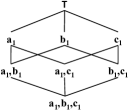
Figure 1: Lattice $\mathcal{C}^{t_{5}}$

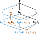
Figure 2: Intersection of $\mathcal{C}^{t_{4}}$ and $\mathcal{C}^{t_{5}}$

Example 6.

Fig.2 shows $\mathcal{C}^{t_{4}}$ and $\mathcal{C}^{t_{5}}$ for $t_{4}$ and $t_{5}$ in Table IV. The constraints connected by solid lines represent the lattice intersection $\mathcal{C}^{t_{4},t_{5}}$. Its bottom is $\bot(\mathcal{C}^{t_{4},t_{5}})$ = $\langle*,b_{1},c_{1}\rangle$. In addition to $\mathcal{C}^{t_{4},t_{5}}$, $\mathcal{C}^{t_{4}}$ and $\mathcal{C}^{t_{5}}$ further include the constraints connected by dashed and dotted lines, respectively.  

The algorithms we are going to propose consider the constraints in certain lattice order, compare $t$ with skyline tuples associated with visited constraints, and use $t$’s dominating tuples to prune unvisited constraints from consideration—thereby reducing cost. This idea of lattice-based pruning of constraints is justified by Propositions 2 and 3 below.

Proposition 2.

Given a tuple $t$, if $t\notin\lambda_{M}(\sigma_{C}(R))$, then $t\notin\lambda_{M}(\sigma_{C^{\prime}}$ $(R))$, for all $C^{\prime}\in\mathcal{A}_{C}$.  

If $t\prec_{M}t^{\prime}$, then $t\notin\lambda_{M}(\sigma_{\bot(\mathcal{C}^{t,t^{\prime}})}(R))$. Hence, according to Proposition 2, we have the following Proposition 3.

Proposition 3.

Given two tuples $t$ and $t^{\prime}$, if $t\prec_{M}t^{\prime}$, then $t\notin\lambda_{M}(\sigma_{C}$ $(R))$, for all $C\in\mathcal{C}^{t,t^{\prime}}$.  

(3)

Sharing computation across measure subspaces   Given $t$, we need to consider not only all constraints satisfied by $t$, but also all possible measure subspaces. Sharing computation across measure subspaces is challenging because of anti-monotonicity of dominance relation—a skyline tuple under space $M$ may or may not be a skyline tuple in another space $M^{\prime}$, regardless of whether $M^{\prime}$ is a superspace or subspace of $M$ [9]. We thus propose algorithms that first traverse the lattice in the full measure space, during which a frontier of constraints is formed for each measure subspace. Top-down (respectively, bottom-up) lattice traversal in a subspace commences from (respectively, stops at) the corresponding frontier instead of the root, which in effect prunes some top constraints.

Two Baseline Algorithms

We introduce two baseline algorithms BaselineSeq (Alg.3) and BaselineIdx. They are not as naive as the brute-force Alg.2. Instead, they exploit Proposition 3 straightforwardly. Upon $t$’s arrival, for each subspace $M$, they identify existing tuples $t^{\prime}$ dominating $t$. BaselineSeq sequentially compares $t$ with every existing tuple. $S$ is initialized to be $\mathcal{C}^{t}$ (Line 3). Whenever BaselineSeq encounters a $t^{\prime}$ that dominates $t$, it removes constraints in $\mathcal{C}^{t,t^{\prime}}$ from $S$ (Line 5). By Proposition 3, $t$ is not in the contextual skylines for those constraints. After $t$ is compared with all tuples, the constraints having $t$ in their skylines remain in $S$. The same is independently repeated for every $M$. The pseudo code of BaselineIdx is similar to Alg.3 and thus omitted. Instead of comparing $t$ with all tuples, BaselineIdx directly finds tuples dominating $t$ by a one-sided range query $\bigwedge_{m_{i}\in M}(m_{i}$$\geq$$t.m_{i})$ using a k-d tree [3] on full measure space $\mathcal{M}$.

V Algorithms

This section starts with algorithms BottomUp (Sec. V-A) and TopDown (Sec. V-B), which exploit the ideas of tuple reduction and constraint pruning. We then extend them to enable sharing of computation across measure subspaces (Sec. V-C).

Based on the tuple-reduction idea (Proposition 1), a new tuple $t$ should be included into a contextual skyline if and only if $t$ is not dominated by any current skyline tuple in the context. Therefore, BottomUp and TopDown store and maintain skyline tuples for each constraint-measure pair $(C,M)$ and compare $t$ with only the skyline tuples. For clarity of discussion, we differentiate between the contextual skyline ($\lambda_{M}(\sigma_{C}(R))$) and the space for storing it ($\mu_{C,M}$), since tuples stored in $\mu_{C,M}$ do not always equal $\lambda_{M}(\sigma_{C}(R))$, by our algorithm design.

The algorithms traverse, for each measure subspace $M$, the lattice of tuple-satisfied constraints $\mathcal{C}^{t}$ by certain order. When a constraint $C$ is visited, the algorithms compare $t$ with the skyline tuples stored in $\mu_{C,M}$. If $t$ is dominated by $t^{\prime}$, then $t$ does not belong to the contextual skyline of constraint-measure pair $(C,M)$. Further, based on the constraint-pruning idea (Proposition 3), $t$ does not belong to the contextual skyline of $(C^{\prime},M)$ for any $C^{\prime}$ satisfied by both $t$ and $t^{\prime}$ (i.e., $C^{\prime}\in\mathcal{C}^{t,t^{\prime}}$). This property allows the algorithms to avoid comparisons with skyline tuples associated with such constraints.

The algorithms differ by how skyline tuples are stored in $\mu_{C,M}$. BottomUp stores a tuple for every constraint that qualifies it as a contextual skyline tuple, while TopDown only stores it for the topmost such constraints. In our ensuing discussion, we use invariants to formalize what must be stored in $\mu_{C,M}$. The algorithms also differ in the traversing order of the constraints in $\mathcal{C}^{t}$. BottomUp visits the constraints bottom-up, while TopDown makes the traversal top-down. Our discussion focuses on how the invariants are kept true under the algorithms’ different traversal orders and execution logics. The algorithms present space-time tradeoffs. TopDown requires less space than BottomUp since it avoids storing duplicate skyline tuples as much as possible. The saving in space comes at the cost of execution efficiency, due to more complex operations in TopDown.

Pei et al. [9] proposed bottom-up and top-down algorithms to compute skycube. However, their algorithms are for the lattice of measure subspaces instead of constraints.

V-A Algorithm BottomUp

Input: $R(\mathcal{M},\mathcal{D})$: existing tuples; $t$: the new tuple

1

Output: $S^{t}$: the contextual skylines for $t$

2

3$S^{t}\leftarrow\varnothing$;

4foreach $M\subseteq\mathcal{M}$ do

5       foreach $C\in\mathcal{C}^{t}$ do $C.\mathit{pruned}\leftarrow\textnormal{{false}}$;

6      

7      $Q\leftarrow\varnothing$; $Q.\mathit{enqueue}(\bot(\mathcal{C}^{t}))$; 

8       while not $Q.\mathit{empty}()$ do

9             $C\leftarrow Q.\mathit{dequeue}()$;

10             $\mathit{dominated}\leftarrow\textnormal{{false}}$;

11             foreach $t^{\prime}\in\mu_{C,M}$ do

12                   if $t\prec_{M}t^{\prime}$ then

13                         $\mathit{dominated}\leftarrow\textnormal{{true}}$;

14                         foreach $C^{\prime}\in\mathcal{A}^{t}_{C}$ do

15                               $C^{\prime}.\mathit{pruned}\leftarrow\textnormal{{true}}$; break;

16                        

17                   else if $t^{\prime}\prec_{M}t$ then  $\mu_{C,M}.\mathit{delete}(t^{\prime})$ ;

18                  

19             if not $\mathit{dominated}$ then

20                   $S^{t}\leftarrow S^{t}\cup\{(C,M)\}$; 

21                   $\mu_{C,M}.\mathit{insert}(t)$; 

22                   foreach $C^{\prime}\in\mathcal{P}^{t}_{C}$ do

23                         if $($not $Q.\mathit{contains}(C^{\prime}))$ and $($not $C^{\prime}.\mathit{pruned})$ then $Q.\mathit{enqueue}(C^{\prime})$;

24                        

25                  

26            

27      

28$R\leftarrow R\cup\{t\}$;

return $S^{t}$;

Algorithm 1 BottomUp

BottomUp (Alg.1) stores a tuple for every such constraint that qualifies it as a contextual skyline tuple. Formally, Invariant 1 is guaranteed to hold before and after the arrival of any tuple.

Invariant 1.

$\forall C\in\mathcal{C}_{\mathcal{D}}$ and $\forall M\subseteq\mathcal{M}$, $\mu_{C,M}$ stores all skyline tuples $\lambda_{M}(\sigma_{C}(R))$.  

Upon the arrival of a new tuple $t$, for each measure subspace $M$, BottomUp traverses the constraints in $\mathcal{C}^{t}$ in a bottom-up, breadth-first manner. The traversal starts from Line 1 of Alg.1, where the bottom of $\mathcal{C}^{t}$ is inserted into a queue $Q$. As long as $Q$ is not empty, BottomUp visits the next constraint $C$ from the head of $Q$ and compares $t$ with current skyline tuples in $\mu_{C,M}$ (Line 1). Various actions are taken, depending on comparison outcome. 1) If $t$ is dominated by any $t^{\prime}$, the comparison with remaining tuples in $\mu_{C,M}$ is skipped (Line 1). The tuple $t$ is disqualified from not only $C$ but also all constraints in $\mathcal{C}^{t,t^{\prime}}$, by Proposition 3. Because BottomUp stores a tuple in all constraints that qualify it as a contextual skyline tuple, and because it traverses $\mathcal{C}^{t}$ bottom-up, the dominating tuple $t^{\prime}$ must be encountered at the bottom of $\mathcal{C}^{t,t^{\prime}}$. BottomUp thus skips the comparisons with all tuples stored for $C$’s ancestors (Line 1). 2) If $t$ dominates $t^{\prime}$, $t^{\prime}$ is removed from $\mu_{C,M}$ (Line 1). 3) If $t$ is not dominated by any tuple in $\mu_{C,M}$, it is inserted into $\mu_{C,M}$ (Line 1) and $(C,M)$ corresponds to a contextual skyline for $t$ (Line 1). Further, each parent constraint of $C$ that is not already pruned is inserted into $Q$, for continuation of bottom-up traversal (Line 1).

Below we prove that Invariant 1 is satisfied by BottomUp throughout its execution over all tuples.

Proof of Invariant 1

We prove by induction on the size of table $R$. Invariant 1 is trivially true when $R$ is empty. If the invariant is true before the arrival of $t$, i.e., $\mu_{C,M}$ stores all tuples in $\lambda_{M}(\sigma_{C}(R))$, we prove that it remains true after the arrival of $t$. The proof entails showing that both insertions into and deletions from $\mu_{C,M}$ are correct.

With regard to insertion, the only place where a tuple can be inserted into $\mu_{C,M}$ is Line 1 of BottomUp, which is reachable if and only if $t$ is not dominated by any tuple in $\mu_{C,M}$ and $C$ belongs to $\mathcal{C}^{t}$. This ensures that $\mu_{C,M}$ stores $t$ if and only if $t\in\lambda_{M}(\sigma_{C}(R))$. Further, it enures that no previous tuple is inserted into $\mu_{C,M}$ upon the arrival of $t$, which is correct since such a tuple was not even in the skyline before.

With regard to deletion, the only place where a previous skyline tuple $t^{\prime}$ can be deleted from $\mu_{C,M}$ is Line 1, which is reachable if and only if $t$ dominates $t^{\prime}$ and $C$ is satisfied by both tuples. This ensures that $t^{\prime}$ is removed from $\mu_{C,M}$ if and only if $t^{\prime}$ is not a skyline tuple anymore.

Hence, regardless of whether insertion/deletion takes place upon $t$’s arrival, $\mu_{C,M}$ stores all tuples in $\lambda_{M}(\sigma_{C}(R))$ afterwards. $\square$

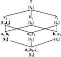
(a) Before $t_{5}$

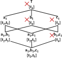
(b) After $t_{5}$

Figure 3: Execution of BottomUp in Measure Subspace $\{m_{1},m_{2}\}$

Example 7.

We use Fig.3 to explain the execution of BottomUp on Table IV, for measure subspace $M$={$m_{1}$,$m_{2}$}. Assume the tuples are inserted into the table in the order of $t_{1}$, $t_{2}$, $t_{3}$, $t_{4}$ and $t_{5}$. Fig.3(a) shows the lattice $\mathcal{C}^{t_{5}}$ before the arrival of $t_{5}$. Beside each constraint $C$, the figure shows $\mu_{C,M}$. Upon the arrival of $t_{5}$, BottomUp starts the traversal of $\mathcal{C}^{t_{5}}$ from its bottom $\bot(\mathcal{C}^{t_{5}})$=$\langle a_{1},b_{1},c_{1}\rangle$. There is one skyline tuple stored in $\mu_{\bot(\mathcal{C}^{t_{5}}),M}$—$t_{2}$. In subspace $M$, $t_{5}$ is incomparable to $t_{2}$. Hence, $t_{5}$ is inserted into it. The traversal continues with the parents of $\bot(\mathcal{C}^{t_{5}})$. Among its three parents, $\langle a_{1},b_{1},*\rangle$ and $\langle a_{1},*,c_{1}\rangle$ undergo the same insertion of $t_{5}$. However, the contextual skyline for $\langle*,b_{1},c_{1}\rangle$ does not change, since $t_{5}$ is dominated by $t_{4}$ in $M$. All constraints in $\mathcal{C}^{t_{4},t_{5}}$ (i.e., $\langle*,b_{1},c_{1}\rangle$ and all its ancestors) are pruned from consideration by Property 3. The traversal continues at $\langle a_{1},*,*\rangle$, for which $t_{1}$ is removed from the contextual skyline as it is dominated by $t_{5}$ in subspace $M$ and $t_{5}$ is inserted into it. After that, the algorithm stops since there is no more unpruned constraints. The content of $\mu_{C,M}$ for constraints in $\mathcal{C}^{t_{5}}$ after the arrival of $t_{5}$ is shown in Fig.3(b).  

V-B Algorithm TopDown

BottomUp stores $t$ for every constraint-measure pair that qualifies $t$ as a contextual skyline tuple. If $t$ is stored in $\mu_{C,M}$, then $t$ is also stored in $\mu_{C^{\prime},M}$ for all $C^{\prime}$$\in$$\mathcal{D}^{t}_{C}$, i.e., descendants of $C$ pertinent to $t$. For this reason, BottomUp repeatedly compares a new tuple with a previous tuple multiple times. Such repetitive storage of tuples and comparisons increase both space complexity and time complexity. On the contrary, TopDown (Alg.2) stores a tuple in $\mu_{C,M}$ only if $C$ is a maximal skyline constraint of the tuple, defined as follows.

Definition 9 (Skyline Constraint).

Given $t\in R(\mathcal{D};\mathcal{M})$ and $M\subseteq\mathcal{M}$, the skyline constraints of $t$ in $M$, denoted $\mathcal{SC}^{t}_{M}$, are the constraints whose contextual skylines include $t$. Formally, $\mathcal{SC}^{t}_{M}=\{C|C\in\mathcal{C}^{t},t\in\lambda_{M}(\sigma_{C}(R))\}$. Correspondingly, other constraints in $\mathcal{C}^{t}$ are non-skyline constraints.  

Definition 10 (Maximal Skyline Constraints).

With regard to $t$ and $M$, a skyline constraint is a maximal skyline constraint if it is not subsumed by any other skyline constraint of $t$. The set of $t$’s maximal skyline constraints is denoted $\mathcal{MSC}^{t}_{M}$. In other words, it includes those skyline constraints for which no parents (and hence ancestors) are skyline constraints. Formally, $\mathcal{MSC}^{t}_{M}=\{C|C\in\mathcal{SC}^{t}_{M}$, and $\nexists C^{\prime}\in\mathcal{A}_{C}\text{ s.t. }C^{\prime}\in\mathcal{SC}^{t}_{M}\}$.  

Input: $R(\mathcal{M},\mathcal{D})$: existing tuples; $t$: the new tuple

1

Output: $S^{t}$: the contextual skylines for $t$

2

3

4$S^{t}\leftarrow\varnothing$;

5foreach $M\subseteq\mathcal{M}$ do

6      foreach $C\in\mathcal{C}^{t}$ do

7           $C.\mathit{pruned}\leftarrow\textnormal{{false}}$;

8           $C.\mathit{inAnces}\leftarrow\textnormal{{false}}$;

9     

10     $Q\leftarrow\varnothing$; $Q.\mathit{enqueue}(\top)$; 

11      while not $Q.\mathit{empty}()$ do

12           $C\leftarrow Q.\mathit{dequeue}()$;

13           foreach $t^{\prime}\in\mu_{C,M}$ do

14                if $t\prec_{M}t^{\prime}$ then

15                     Dominated$(t^{\prime},C)$;

16                else if $t^{\prime}\prec_{M}t$ then

17                     Dominates$(t^{\prime},C,M)$;

18               

19           if not $C.\mathit{pruned}$ then

20                $S^{t}\leftarrow S^{t}\cup\{(C,M)\}$; 

21                if not $C.\mathit{inAnces}$ then

22                     $\mu_{C,M}.\mathit{insert}(t)$; 

23                    

24               

25          EnqueueChindren$(C)$;

26     

27$R\leftarrow R\cup\{t\}$;

28return $S^{t}$;

29

30

1

Procedure: Dominates $(t^{\prime},C,M)$

2

3$\mu_{C,M}.\mathit{delete}(t^{\prime})$;

4 foreach $C^{\prime}\in\mathcal{CH}^{t^{\prime}}_{C}-\mathcal{C}^{t}$ do

5      $\mathit{stored}\leftarrow\textnormal{{false}}$;

6      foreach $C^{\prime\prime}\in\mathcal{A}^{t^{\prime}}_{C^{\prime}}-\mathcal{C}^{t}$ do

7           if $t^{\prime}\in\mu_{C^{\prime\prime},M}$ then

8                $\mathit{stored}\leftarrow\textnormal{{true}}$;

9                break;

10               

11          

12     if not $\mathit{stored}$ then

13           $\mu_{C^{\prime},M}.\mathit{insert}(t^{\prime})$; 

14          

15     

16

1 

Procedure: Dominated $(t^{\prime},C)$

2

3$C.\mathit{pruned}\leftarrow\textnormal{{true}}$;

4foreach $C^{\prime}\in\mathcal{C}^{t,t^{\prime}}$ do

5      $C^{\prime}.\mathit{pruned}\leftarrow\textnormal{{true}}$;

6

1 

Procedure: EnqueueChildren $(C)$

2

3foreach $C^{\prime}\in\mathcal{CH}^{t}_{C}$ do

4      if not $C.\mathit{pruned}$ then

5           $C^{\prime}.\mathit{inAnces}\leftarrow\textnormal{{true}}$;

6     if not $Q.\mathit{contains}(C^{\prime})$ then

7           $Q.\mathit{enqueue}(C^{\prime})$;

8     

Algorithm 2 TopDown

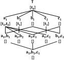
(a) Before $t_{5}$

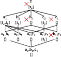
(b) After $t_{5}$

Figure 4: Execution of TopDown in Measure Subspace $\{m_{1},m_{2}\}$

Example 8.

Fig.3(b) shows, in measure subspace $\{m_{1}$,$m_{2}\}$, $t_{5}$ is in the contextual skylines of $4$ constraints, i.e., $\mathcal{SC}^{t_{5}}_{\{m_{1},m_{2}\}}$ $=$ {$\langle$$a_{1}$,$*,*$$\rangle$,$\langle$$a_{1}$,$b_{1}$,$*$$\rangle$,$\langle$$a_{1}$,$*$,$c_{1}$$\rangle$,$\langle$$a_{1}$,$b_{1}$,$c_{1}$$\rangle$}. Its maximal skyline constraints are $\{\langle$$a_{1}$,$*$,$*$$\rangle\}$, i.e., $\mathcal{MSC}^{t_{5}}_{\{m_{1},m_{2}\}}$$=$$\{$$\langle$$a_{1}$,$*$,$*$$\rangle$$\}$.  

Formally, Invariant 2 is guaranteed by TopDown before and after the arrival of any tuple.

Invariant 2.

$\forall C\in\mathcal{C}_{\mathcal{D}}$ and $\forall M\subseteq\mathcal{M}$, $\mu_{C,M}$ stores a tuple $t$ if and only if $C\in\mathcal{MSC}^{t}_{M}$.  

Different from BottomUp, TopDown stores a tuple in its maximal skyline constraints $\mathcal{MSC}^{t}_{M}$ instead of all skyline constraints $\mathcal{SC}^{t}_{M}$. Due to this difference, TopDown traverses $\mathcal{C}^{t}$ in a top-down (instead of bottom-up) breadth-first manner. The traversal starts from Line 2 of Alg.2, where the top element $\top$ is inserted into a queue $Q$. As long as $Q$ is not empty, the algorithm visits the next constraint $C$ from the head of $Q$ and compares $t$ with current skyline tuples in $\mu_{C,M}$ (Line 2). Various actions are taken, depending on the comparison result:

1) If $t$ is dominated by $t^{\prime}$, $t$ is disqualified from not only $C$ but also all constraints in $\mathcal{C}^{t,t^{\prime}}$, by Proposition 3. The pruning is done by calling Dominated in Line 2 which sets $C^{\prime}.pruned$ to true for every pruned constraint $C^{\prime}$. Since $C$ is a maximal skyline constraint for $t^{\prime}$, the pruned constraints are all descendants of $C$ in $\mathcal{C}^{t,t^{\prime}}$. Note that TopDown cannot skip the comparisons with the remaining tuples stored in $\mu_{C,M}$. The reason is that there might be $t^{\prime\prime}$ in $\mu_{C,M}$ such that i) $t^{\prime\prime}$ also dominates $t$ and ii) $t^{\prime\prime}$ and $t$ share some dimension attribute values that are not shared by $t^{\prime}$, i.e., $\mathcal{C}^{t,t^{\prime\prime}}$$-$$\mathcal{C}^{t,t^{\prime}}$$\neq$$\varnothing$. Since $t^{\prime\prime}$ is only stored in its maximal skyline constraints, skipping the comparison with $t^{\prime\prime}$ may incorrectly establish $t$ as a contextual skyline tuple for those constraints in $\mathcal{C}^{t,t^{\prime\prime}}$$-$$\mathcal{C}^{t,t^{\prime}}$.

2) If $t$ dominates a current tuple $t^{\prime}$, $t^{\prime}$ is removed from $\mu_{C,M}$ by calling Dominates (Line 2). An extra work is to update the maximal skyline constraints of $t^{\prime}$ and store $t^{\prime}$ in descendants of $C$ if necessary (Lines 2-9 of Dominates). If $C$ has a child $C^{\prime}$ satisfied by $t^{\prime}$ but not $t$, $C^{\prime}$ is a skyline constraint of $t^{\prime}$. Further, $C^{\prime}$ is a maximal skyline constraint of $t^{\prime}$, if no ancestor of $C^{\prime}$ is already a maximal skyline constraint of $t^{\prime}$.

3) If $t$ is not dominated by any tuple in $\mu_{C,M}$ and $C$ was not pruned before when its ancestors were visited, $(C,M)$ corresponds to a contextual skyline for $t$ (Line 2). If $t$ was not already stored in $C$’s ancestors (indicated by $C.\mathit{inAnces}$), then $C$ is a maximal skyline constraint and thus $t$ is inserted into $\mu_{C,M}$ (Line 2).

Furthermore, subroutine EnqueueChildren is called for continuation of top-down traversal (Line 2). It inserts each child constraint $C^{\prime}$ of $C$ into $Q$. If $t$ is stored in $\mu_{C,M}$ or any of its ancestors, $C^{\prime}.\mathit{inAnces}$ is set to true and $t$ will not be stored again in $\mu(C^{\prime},M)$ when the traversal reaches $C^{\prime}$.

Below we prove that Invariant 2 is satisfied by TopDown throughout its execution over all tuples.

Proof of Invariant 2

We prove by induction on the size of table $R$. If the invariant is true before $t$’s arrival, i.e., $\mu_{C,M}$ stores a tuple $t$ if and only if $C$$\in$$\mathcal{MSC}^{t}_{M}$, we prove that it is kept true after the arrival of $t$. The proof constitutes showing that both insertions into and deletions from $\mu_{C,M}$ are correct.

With regard to insertion, there are two places where a tuple can be inserted. 1) In Line 2 of TopDown, $t$ is inserted into $\mu_{C,M}$. This line is reachable if and only if i) $C$ is satisfied by $t$, ii) $t$ is not dominated by any tuple stored at $C$ or $C$’s ancestors, and iii) $t$ is not already stored at any of $C$’s ancestors. This ensures that $\mu_{C,M}$ stores $t$ if and only if $C$ is a maximal skyline constraint of $t$, i.e., $C\in\mathcal{MSC}^{t}_{M}$. 2) In Line 2 of Dominates, $t^{\prime}$ is inserted into $\mu_{C^{\prime},M}$. This line is reachable if and only if i) $t$ dominates $t^{\prime}$, ii) $C$, which is a parent of $C^{\prime}$, is satisfied by both tuples, iii) $C^{\prime}$ is satisfied by $t^{\prime}$ but not $t$, and iv) $t^{\prime}$ is not stored at any ancestor of $C^{\prime}$. Since $C$ was a maximal skyline constraint of $t^{\prime}$ before the arrival of $t$, $C^{\prime}$ must be a skyline constraint of $t$. Therefore these conditions ensure that $\mu_{C^{\prime},M}$ stores $t^{\prime}$ if and only if $C^{\prime}$ becomes a maximal skyline constraint of $t^{\prime}$.

With regard to deletion, the only place where a previous skyline tuple $t^{\prime}$ can be deleted from $\mu_{C,M}$ is Line 2 of Dominates, which is reachable if and only if $t$ dominates $t^{\prime}$ and $C$ is satisfied by both tuples. This ensures that $t^{\prime}$ is removed from $\mu_{C,M}$ if and only if $C$ is not a maximal skyline constraint of $t^{\prime}$ anymore.

Therefore, regardless of whether any insertion or deletion takes place upon the arrival of $t$, afterwards $\mu_{C,M}$ stores all tuples for which $C$ is a maximal skyline constraint. $\square$

Input: $R(\mathcal{M},\mathcal{D})$: existing tuples; $t$: the new tuple

1

Output: $S^{t}$: the contextual skylines for $t$

2

3

4$S^{t}\leftarrow$ STopDownRoot$()$;

5foreach $M\subset\mathcal{M}$ do

6      $S^{t}\leftarrow S^{t}\cup$ STopDownNode$(M)$;

7

8$R\leftarrow R\cup\{t\}$;

9return $S^{t}$;

10

1 

Procedure: STopDownRoot $()$

2

3$S^{t}\leftarrow\varnothing$;

4foreach $C\in\mathcal{C}^{t}$ do

5      $C.\mathit{pruned}\leftarrow\textnormal{{false}}$;

6      $C.\mathit{inAnces}\leftarrow\textnormal{{false}}$;

7      foreach $M\subset\mathcal{M}$ do

8           $\mathit{pruned}[C][M]\leftarrow\textnormal{{false}}$;

9     

10

11$Q\leftarrow\varnothing$; $Q.\mathit{enqueue}(\top)$;

12while not $Q.\mathit{empty}()$ do

13      $C\leftarrow Q.\mathit{dequeue}()$;

14      foreach $t^{\prime}\in\mu_{C,\mathcal{M}}$ do

15           if $t\prec_{\mathcal{M}}t^{\prime}$ then Dominated$(t^{\prime},C)$;

16          

17          else if $t^{\prime}\prec_{\mathcal{M}}t$ then Dominates$(t^{\prime}$,$C$,$\mathcal{M})$;

18          

19          foreach $M\subset\mathcal{M}$ do

20                if $t\prec_{M}t^{\prime}$ (Proposition 4) then

21                     foreach $C^{\prime}\in\mathcal{C}^{t,t^{\prime}}$ do

22                          $\mathit{pruned}[C^{\prime}][M]\leftarrow\textnormal{{true}}$;

23                    

24               

25          

26      if not $C.\mathit{pruned}$ then

27           $S^{t}\leftarrow S^{t}\cup\{(C,\mathcal{M})\}$;

28           if not $C.\mathit{inAnces}$ then

29                $\mu_{C,\mathcal{M}}.\mathit{insert}(t)$;

30               

31          

32     

33     EnqueueChildren$(C)$;

34return $S^{t}$;

1

Procedure: STopDownNode $(M)$

2

3$S^{t}\leftarrow\varnothing$;

4foreach $C\in\mathcal{C}^{t}$ do

5      $C.\mathit{pruned}\leftarrow\mathit{pruned}[C][M]$;

6      $C.\mathit{inAnces}\leftarrow\textnormal{{false}}$;

7

8$Q\leftarrow\varnothing$; $Q.\mathit{enqueue}(\top)$;

9while not $Q.\mathit{empty}()$ do

10      $C\leftarrow Q.\mathit{dequeue}()$;

11     if not $C.\mathit{pruned}$ then

12           $S^{t}\leftarrow S^{t}\cup\{(C,M)\}$;

13           foreach $t^{\prime}\in\mu_{C,M}$ do

14                if $t^{\prime}\prec_{M}t$ then Dominates$(t^{\prime},C,M)$;

15               

16          if not $C.\mathit{inAnces}$ then

17                $\mu_{C,M}.\mathit{insert}(t)$; 

18               

19          

20     EnqueueChildren$(C)$;

21return $S^{t}$;

Algorithm 3 STopDown

Example 9.

We use Fig.4 to explain the execution of TopDown on Table IV for $M$={$m_{1}$,$m_{2}$}. Again, assume the tuples are inserted into the table in the order of $t_{1}$, $t_{2}$, $t_{3}$, $t_{4}$ and $t_{5}$. Fig.4(a) shows $\mu_{C,M}$ beside each constraint $C$ in $\mathcal{C}^{t_{5}}$ before the arrival of $t_{5}$. A tuple is only stored in its maximal skyline constraints. The figure also shows constraints outside of $\mathcal{C}^{t_{5}}$ where various tuples are also stored. The maximal skyline constraints for $t_{2}$ and $t_{4}$ are $\langle a_{1},*,*\rangle$ and $\top$, respectively. The maximal skyline constraints for $t_{1}$ include $\langle a_{1},*,*\rangle$ and $\langle*,b_{2},*\rangle$. For $t_{3}$, the only maximal skyline constraint is $\langle*,*,c_{2}\rangle$.

Upon the arrival of $t_{5}$, TopDown starts to traverse $\mathcal{C}^{t_{5}}$ from $\top$. Only $t_{4}$ is stored in $\mu_{\top,M}$. In $M$, $t_{5}$ is dominated by $t_{4}$, thus $\mu_{\top,M}$ does not change and $t_{5}$ does not belong to the contextual skylines of the constraints in $\mathcal{C}^{t_{4},t_{5}}$—$\langle*,b_{1},c_{1}\rangle$, $\langle*,*,c_{1}\rangle$, $\langle*,b_{1},*\rangle$ and $\top$. The traversal continues with the children of $\top$. Among its three children, $\langle*,b_{1},*\rangle$ and $\langle*,*,c_{1}\rangle$ do not store any tuple, and $t_{1}$ and $t_{2}$ are stored at $\langle a_{1},*,*\rangle$. They do not dominate $t_{5}$ in $M$. Since $t_{5}$ was not stored in any of its ancestors, $\langle a_{1},*,*\rangle$ is a maximal skyline constraint of $t_{5}$. Hence, $t_{5}$ is inserted into it and will not be stored at its descendants $\langle a_{1},b_{1},*\rangle$, $\langle a_{1},*,c_{1}\rangle$ and $\langle a_{1},b_{1},c_{1}\rangle$. Since $t_{5}$ dominates $t_{1}$, $t_{1}$ is deleted from $\langle a_{1},*,*\rangle$. To update the maximal skyline constraints of $t_{1}$, TopDown considers the two children of $\langle a_{1},*,*\rangle$—$\langle a_{1},b_{2},*\rangle$ and $\langle a_{1},*,c_{2}\rangle$. $\langle a_{1},b_{2},*\rangle$ is not a new maximal skyline constraint, since $t_{1}$ is already stored at its ancestor $\langle*,b_{2},*\rangle$. $\langle a_{1},*,c_{2}\rangle$ becomes a new maximal skyline constraint since it is not subsumed by any existing maximal skyline constraint of $t_{1}$. Thus $t_{1}$ is stored at $\langle a_{1},*,c_{2}\rangle$. TopDown continues to the end and finds no tuple at any remaining constraint in $\mathcal{C}^{t_{5}}$. Fig.4(b) depicts the content of $\mu_{C,M}$ for relevant constraints after $t_{5}$’s arrival.  

V-C Sharing across Measure Subspaces

Given a new tuple, both TopDown and BottomUp compute its contextual skylines in each measure subspace separately, without sharing computation across different subspaces. As mentioned in Sec. IV, the challenge in such sharing lies in the anti-monotonicity of dominance relation—with regard to the same context of tuples, a skyline tuple in space $M$ may or may not be a skyline tuple in another space $M^{\prime}$, regardless of whether $M^{\prime}$ is a superspace or subspace of $M$ [9]. To share computation across different subspaces, we devise algorithms STopDown and SBottomUp. They discover the contextual skylines in all subspaces by leveraging initial comparisons in the full measure space $\mathcal{M}$. In this section, we first introduce STopDown and then briefly explain SBottomUp, which is based on similar principles.

With regard to two tuples $t$ and $t^{\prime}$, the measure space $\mathcal{M}$ can be partitioned into three disjoint sets $\mathcal{M}^{>}$, $\mathcal{M}^{<}$ and $\mathcal{M}^{=}$ such that 1) $\forall m$$\in$$\mathcal{M}^{>}$, $t.m$$>$$t^{\prime}.m$; 2) $\forall m$$\in$$\mathcal{M}^{<}$, $t.m$$<$$t^{\prime}.m$; and 3) $\forall m$$\in$$\mathcal{M}^{=}$, $t.m$$=$$t^{\prime}.m$. Then, $t$ is dominated by $t^{\prime}$ in a subspace $M$ if and only if $M$ contains at least one attribute in $\mathcal{M}^{<}$ and no attribute in $\mathcal{M}^{>}$, as stated by Proposition 4.

Proposition 4.

In a measure subspace $M\subseteq\mathcal{M}$, $t\prec_{M}t^{\prime}$ if and only if $M\cap\mathcal{M}^{<}\neq\varnothing$ and $M\cap\mathcal{M}^{>}=\varnothing$.  

The gist of STopDown (Alg.3) is to compare a new tuple $t$ with current tuples $t^{\prime}$ in full space $\mathcal{M}$ and, using Proposition 4, identify all subspaces $M$ in which $t^{\prime}$ dominates $t$. It starts by finding the skyline constraints in $\mathcal{M}$ using STopDownRoot, which is similar to TopDown except Lines 3-3. While traversing a constraint $C$, $t$ is compared with the tuples in $\mu_{C,\mathcal{M}}$ (Line 3 of STopDownRoot). By Proposition 4, all subspaces $M$ where $t^{\prime}$ dominates $t$ are identified. In each such $M$, constraints in $\mathcal{C}^{t,t^{\prime}}$ are pruned (Lines 3-3)—indicated by setting values in a two-dimensional matrix $\mathit{pruned}$. After finishing STopDownRoot, for each $M$, the constraints $C$ satisfying $\mathit{pruned}[C][M]=\textnormal{{false}}$ are the skyline constraints of $t$ in $M$. STopDown then continues to traverse these skyline constraints in $M$ by calling STopDownNode$(M)$, for two purposes—one is to store $t$ at its maximal skyline constraints (Line 3 of STopDownNode), the other is to remove tuples dominated by $t$ and update their maximal skyline constraints (Line 3).

Example 10.

We explain STopDown’s execution on Table IV. In full space $\mathcal{M}$=$\{m_{1},m_{2}\}$, STopDown and TopDown work the same. Hence, Fig.4 shows $\mu_{C,\mathcal{M}}$ beside each $C$ in $\mathcal{C}^{t_{5}}$ before and after $t_{5}$ arrives. Comparisons with tuples in $\mathcal{M}$ also help to prune constraints in subspaces. Consider $\top$ in Fig.4(a), where $t_{4}$ is stored. The new tuple $t_{5}$ is compared with $t_{4}$. The outcome is $\mathcal{M}^{>}$=$\varnothing$, $\mathcal{M}^{<}$=$\{m_{1},m_{2}\}$ and $\mathcal{M}^{=}$=$\varnothing$, since $t_{5}$ is smaller than $t_{4}$ on both $m_{1}$ and $m_{2}$. By Proposition 4, $t_{5}$ is dominated by $t_{4}$ in subspaces $\{m_{1}\}$ and $\{m_{2}\}$. Hence, all constraints in $\mathcal{C}^{t_{4},t_{5}}$ (including $\langle*,b_{1},c_{1}\rangle$, $\langle*,b_{1},*\rangle$, $\langle*,*,c_{1}\rangle$ and $\top$) are pruned in $\{m_{1}\}$ and $\{m_{2}\}$ simultaneously, by Lines 3-3 of STopDownRoot. As STopDownRoot proceeds, $t_{5}$ is also compared with $t_{1}$ and $t_{2}$. With regard to the comparison with $t_{1}$, since $\mathcal{M}^{<}$=$\varnothing$, $t_{5}$ is not dominated by $t_{1}$ in any space. With regard to $t_{2}$, $\mathcal{M}^{>}$=$\{m_{2}\}$, $\mathcal{M}^{<}$=$\{m_{1}\}$ and $\mathcal{M}^{=}$=$\varnothing$. Thus $t_{5}$ is dominated by $t_{2}$ in $\{m_{1}\}$. Hence, all the constraints in $\mathcal{C}^{t_{2},t_{5}}$, which is identical to $\mathcal{C}^{t_{5}}$, are pruned in $\{m_{1}\}$.

After the traversal in $\mathcal{M}$, STopDown continues with each measure subspace. In $\{m_{1}\}$, all constraints of $\mathcal{C}^{t_{5}}$ are pruned. Hence, $t_{5}$ has no skyline constraint and nothing further needs to be done. Fig.5 depicts $\mu_{C,\{m_{1}\}}$ for all $C$ in $\mathcal{C}^{t_{5}}$ before and after the arrival of $t_{5}$. For $\{m_{2}\}$, Fig.6(a) depicts $\mu_{C,\{m_{2}\}}$ for all $C$ in $\mathcal{C}^{t_{5}}$ before the arrival of $t_{5}$. Based on the analysis above, the skyline constraints of $t_{5}$ in $\{m_{2}\}$ include $\langle a_{1},*,*\rangle$, $\langle a_{1},b_{1},*\rangle$, $\langle a_{1},*,c_{1}\rangle$ and $\langle a_{1},b_{1},c_{1}\rangle$. Since non-skyline constraints are pruned, $t_{5}$ is not compared with the tuples stored at those constraints. Instead, $t_{5}$ is compared with $t_{1}$ stored at $\langle a_{1},*,*\rangle$. Since they do not dominate each other in $\{m_{2}\}$, $\langle a_{1},*,*\rangle$ is a maximal skyline constraint of $t_{5}$ and $t_{5}$ is stored at it together with $t_{1}$. The content of $\mu_{C,\{m_{2}\}}$ in $\mathcal{C}^{t_{5}}$ after encountering $t_{5}$ is in Fig.6(b). Note that TopDown would have compared $t_{5}$ with other tuples seven times, including comparisons with $t_{1}$, $t_{2}$ and $t_{5}$ in $\{m_{1},m_{2}\}$, with $t_{2}$ and $t_{4}$ in $\{m_{1}\}$, and with $t_{1}$ and $t_{4}$ in $\{m_{2}\}$. In contrast, STopDown needs four comparisons, including the same three comparisons in $\{m_{1},m_{2}\}$ and another comparison with $t_{1}$ in $\{m_{2}\}$.  

Invariant 2 is also guaranteed by STopDown all the time. We omit the proof which is largely the same as the proof for TopDown. We note the essential difference between STopDown and TopDown is the skipping of non-skyline constraints in measure subspaces. Since the new tuple is dominated under these constraints, it does not and should not make any change to $\mu_{C,M}$ for any such constraint-measure pair.

BottomUp is extended to SBottomUp, similar to how STopDown extends TopDown. While in STopDown lattice traversal in a measure subspace commences from the topmost skyline constraints instead of the root of a lattice, lattice traversal in SBottomUp stops at them. Invariant 1 is also warranted by SBottomUp. Its proof is similar to that for BottomUp. Due to space limitations, we do not further discuss SBottomUp.

(a) Before Visiting $\mathcal{C}^{t_{5}}$ in $\{m_{1}\}$

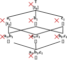
(b) After Visiting $\mathcal{C}^{t_{5}}$ in $\{m_{1}\}$

Figure 5: Execution of STopDown in Measure Subspace $\{m_{1}\}$ (No Comparison Required and No Change Made)

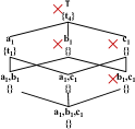
(a) Before Visiting $\mathcal{C}^{t_{5}}$ in $\{m_{2}\}$

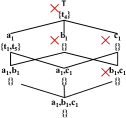
(b) After Visiting $\mathcal{C}^{t_{5}}$ in $\{m_{2}\}$

Figure 6: Execution of STopDown in Measure Subspace $\{m_{2}\}$

VI Experiments

The algorithms were implemented in Java. The experiments were conducted on a computer with $2.0$ GHz Quad Core 2 Duo Xeon CPU running Ubontu 8.10. The limit on the heap size of Java Virtual Machine (JVM) was set to $16$ GB.

VI-A Experiment Setup

Datasets   We used two real datasets, which exhibit similar trends. We mainly discuss the results on the NBA dataset.

NBA Dataset   We collected $317{,}371$ tuples of NBA box scores from 1991-2004 regular seasons. We considered $8$ dimension attributes: player, position, college, state, season, month, team and opp_team. College denotes from where a player graduated, if applicable. State records the player’s state of birth. For measure attributes, $7$ performance statistics were considered: points, rebounds, assists, blocks, steals, fouls and turnovers. Smaller values are preferred on turnovers and fouls, while larger values are preferred on all other attributes.

Weather Dataset (http://data.gov.uk/metoffice-data-archive)   It has more than $7.8$ million daily weather forecast records collected from $5{,}365$ locations in six countries and regions of UK from Dec. 2011 to Nov. 2012. Each record has $7$ dimension attributes: location, country, month, time step, wind direction [day], wind direction [night] and visibility range and $7$ measure attributes: wind speed [day], wind speed [night], temperature [day], temperature [night], humidity [day], humidity [night] and wind gust. We assumed larger values dominate smaller values on all attributes.

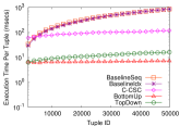
(a) Varying $n$, $d$=$5$, $m$=$7$

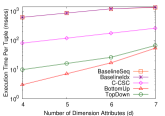
(b) Varying $d$, $n$=$50{,}000$, $m$=$7$

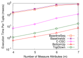
(c) Varying $m$, $n$=$50{,}000$, $d$=$5$

Figure 7: Execution Time of BaselineSeq, BaselineIdx, C-CSC, BottomUp and TopDown on the NBA Dataset

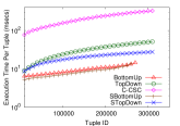
(a) Varying $n$, $d$=$5$, $m$=$7$

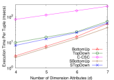
(b) Varying $d$, $n$=$50{,}000$, $m$=$7$

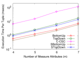
(c) Varying $m$, $n$=$50{,}000$, $d$=$5$

Figure 8: Execution Time of C-CSC, BottomUp, TopDown, SBottomUp, STopDown on NBA dataset

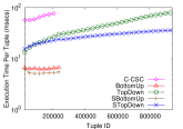
Figure 9: Execution Time on the Weather Dataset, Varying $n$, $d$=$5$, $m$=$7$

Methods Compared   We investigated the performance of $7$ algorithms—the baseline algorithms BaselineSeq and BaselineIdx from Sec. IV, C-CSC which is the CSC adaptation described in Sec. II, and the algorithms BottomUp, TopDown, SBottomUp and STopDown from Sec. V. We compared these algorithms on both execution time and memory consumption.

Parameters   We ran our experiments under combinations of five parameters, which are number of dimension attributes ($d$), number of measure attributes ($m$), number of tuples ($n$), maximum number of bound dimension attributes ($\hat{d}$) and maximum number of measure attributes allowed in measure subspaces ($\hat{m}$). In Table V (VI), we list the dimension (measure) spaces considered for different values of $d$ ($m$), which are subsets of the aforementioned dimension (measure) attributes in the datasets.

$d$	dimension space $\mathcal{D}$
$4$	$\textsf{\footnotesize player},\ \textsf{\footnotesize season},\ \textsf{\footnotesize team},\ \textsf{\footnotesize opp\_team}$
$5$	$\textsf{\footnotesize player},\ \textsf{\footnotesize season},\ \textsf{\footnotesize month},\ \textsf{\footnotesize team},\ \textsf{\footnotesize opp\_team}$
$6$	$\textsf{\footnotesize position},\ \textsf{\footnotesize college},\ \textsf{\footnotesize state},\ \textsf{\footnotesize season},\ \textsf{\footnotesize team},\ \textsf{\footnotesize opp\_team}$
$7$	$\textsf{\footnotesize position},\ \textsf{\footnotesize college},\ \textsf{\footnotesize state},\ \textsf{\footnotesize season},\ \textsf{\footnotesize month},\ \textsf{\footnotesize team},\ \textsf{\footnotesize opp\_team}$

TABLE V: Dimension Spaces for Different Values of $d$

$m$	measure space $\mathcal{M}$
$4$	$\textsf{\footnotesize points},\ \textsf{\footnotesize rebounds},\ \textsf{\footnotesize assists},\ \textsf{\footnotesize blocks}$
$5$	$\textsf{\footnotesize points},\ \textsf{\footnotesize rebounds},\ \textsf{\footnotesize assists},\ \textsf{\footnotesize blocks},\ \textsf{\footnotesize steals}$
$6$	$\textsf{\footnotesize points},\ \textsf{\footnotesize rebounds},\ \textsf{\footnotesize assists},\ \textsf{\footnotesize blocks},\ \textsf{\footnotesize steals},\ \textsf{\footnotesize fouls}$
$7$	$\textsf{\footnotesize points},\ \textsf{\footnotesize rebounds},\ \textsf{\footnotesize assists},\ \textsf{\footnotesize blocks},\ \textsf{\footnotesize steals},\ \textsf{\footnotesize fouls}$, turnovers

TABLE VI: Measure Spaces for Different Values of $m$

In particular dimension/measure spaces (corresponding to $d$/$m$ values), experiments were done for varying $\hat{d}$ and $\hat{m}$ values. A constraint with more bound dimension attributes represents a more specific context. Similarly, a measure subspace with more measure attributes is more specific. Considering all possible constraint-measure pairs may thus produce many over-specific and uninteresting facts. The parameters $\hat{d}$ and $\hat{m}$ are for avoiding trivial facts. For instance, if $d$=$5$, $m$=$4$, $\hat{d}$=$2$ and $\hat{m}$=$3$, we consider all constraints with at most $2$ (out of $5$) bound dimension attributes and all measure subspaces with at most $3$ (out of $4$) measure attributes. In all experiments in this section, we set $\hat{d}=4$ and $\hat{m}=m$. That means a constraint is allowed to have up to $4$ bound attributes and a measure subspace can be any subspace of the whole space $\mathcal{M}$ including $\mathcal{M}$ itself. In Sec. VII, we further study how prominence of facts varies by $\hat{d}$ and $\hat{m}$ values.

VI-B Results of Memory-Based Implementation

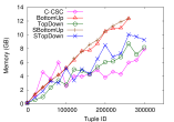
(a) Size of Consumed Memory

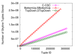
(b) Num of Skyline Tuples Stored

Figure 10: Memory Consumption by C-CSC, BottomUp, TopDown, SBottomUp, STopDown on the NBA Dataset, Varying $n$, $d$=$5$, $m$=$7$

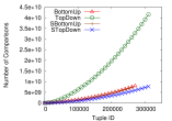
(c) Number of Comparisons

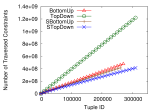
(d) Num of Traversed Constraints

Figure 11: Work Done by BottomUp, TopDown, SBottomUp and STopDown on the NBA Dataset, Varying $n$, $d$=$5$, $m$=$7$

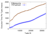
(a) Varying $n$, $d$=$5$, $m$=$7$

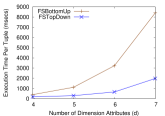
(b) Varying $d$, $n$=$5{,}000$, $m$=$7$

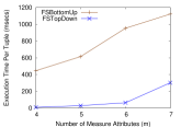
(c) Varying $m$, $n$=$5{,}000$, $d$=$5$

Figure 12: Execution Time of FSBottomUp and FSTopDown on the NBA Dataset

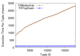
Figure 13: Execution Time of FSBottomUp and FSTopDown on the Weather Dataset, Varying $n$, $d$=$5$, $m$=$7$

Fig.7 compares the per-tuple execution times (by milliseconds, in logarithmic scale) of BaselineSeq, BaselineIdx, C-CSC, BottomUp and TopDown on the NBA dataset. Fig.7(a) shows how the per-tuple execution times increase as the algorithms process tuples sequentially by their timestamps. The values of $d$ and $m$ are $d$=$5$ and $m$=$7$. Fig.7(b) shows the times under varying $d$, given $n$=$50{,}000$ and $m$=$7$. Fig.7(c) is for varying $m$, $n$=$50{,}000$ and $d$=$5$. The figures demonstrate that BottomUp and TopDown outperformed the baselines by orders of magnitude and C-CSC by one order of magnitude. Furthermore, Fig.7(b) and Fig.7(c) show that the execution time of all these algorithms increased exponentially by both $d$ and $m$, which is not surprising since the space of possible constraint-measure pairs grows exponentially by dimensionality.

Fig.9 uses the same configurations in Fig.7 to compare C-CSC, BottomUp, TopDown, SBottomUp and STopDown. We make the following observations on the results. First, C-CSC was outperformed by one order of magnitude. The per-tuple execution times of all algorithms exhibited moderate growth with respect to $n$ and superlinear growth with respect to $d$ and $m$, matching the observations from Fig.7.

Second, in Fig.8(a), the bottom-up algorithms exhausted available JVM heap and were terminated due to memory overflow before all tuples were consumed. On the contrary, the top-down algorithms finished all tuples. This difference was more clear on the larger weather dataset (Fig.9), on which the bottom-up algorithms caused memory overflow shortly after $0.2$ million tuples were encountered, while the top-down algorithms were still running normally after $0.9$ million tuples. As the difference was already clear after $0.9$ million tuples, we terminated the executions of top-down algorithms at that point. The difference in the sizes of consumed memory by these two categories of algorithms is shown in Fig.10(a). The difference in memory consumption is due to that TopDown/STopDown only store a skyline tuple at its maximal skyline constraints, while BottomUp/SBottomUp store it at all skyline constraints. This observation is verified by Fig.10(b), which shows how the number of stored skyline tuples increases by $n$. We see that BottomUp/SBottomUp stored several times more tuples than TopDown/STopDown. Note that TopDown and STopDown use the same skyline tuple materialization scheme. Correspondingly BottomUp and SBottomUp store tuples in the same way.

Fig.9 also shows that, for the weather dataset, C-CSC could not proceed shorty after 0.2 million tuples were processed. This was also due to memory overflow caused by C-CSC, since it needs to store skyline tuples in their “minimum subspaces”. C-CSC did not exhaust memory when it processed the NBA dataset (Fig.8(a)), since there were less skyline tuples in the smaller dataset.

Third, in terms of execution time, TopDown/STopDown were outperformed by BottomUp/SBottomUp. The reason is, if a new tuple $t$ dominates a previous tuple $t^{\prime}$ in constraint $C$ and measure subspace $M$, TopDown/STopDown must update $\mathcal{MSC}^{t^{\prime}}_{M}$. On the contrary, BottomUp/SBottomUp do not carry this overhead; they only need to delete $t^{\prime}$ from $\mu_{C,M}$. Thus, there is a space-time tradeoff between the top-down and bottom-up strategies.

Finally, SBottomUp/STopDown are faster than BottomUp / TopDown, which is the benefit of sharing computation across measure subspaces. Figs.8(b) and 8(c) show that this benefit became more prominent with the increase of both $d$ and $m$. Fig.11 further presents the amount of work done by these algorithms, in terms of compared tuples (Fig.10(c)) and traversed constraints (Fig.10(d)). There are substantial differences between TopDown and STopDown, but the differences between BottomUp and SBottomUp are insignificant. The reason is as follows. STopDown avoids visiting pruned non-skyline constraints, which TopDown cannot avoid. Although SBottomUp avoids such non-skyline constraints too, BottomUp also avoids most of them. The difference between BottomUp and SBottomUp is that BottomUp still visits the boundary non-skyline constraints that are parents of skyline constraints and then skips their ancestors, while SBottomUp skips all non-skyline constraints. Such a difference on boundary non-skyline constraints is not significant.

VI-C Results of File-Based Implementation

The memory-based implementations of all algorithms store skyline tuples for all combinations of constraints and measure subspaces. As a dataset grows, sooner or later, all algorithms will lead to memory overflow. To address this, we investigated file-based implementations of STopDown and SBottomUp, denoted FSTopDown and FSBottomUp, respectively. We did not include C-CSC in this experiment since Figs.7-11 clearly show TopDown/STopDown is one order of magnitude faster than C-CSC and consumes about the same amount of memory.

In the file-based implementations, each non-empty $\mu_{C,M}$ is stored as a binary file. Since the size of $\mu_{C,M}$ for any particular constraint-measure pair $(C,M)$ is small, all tuples in the corresponding file are read into a memory buffer when the pair is visited. Insertion and deletion on $\mu_{C,M}$ are then performed on the buffer. When an algorithm finishes process the pair, the file is overwritten by the buffer’s content.

Fig.13 uses the same configurations in Figs.7 and 9 to compare the per-tuple execution times of FSBottomUp and FSTopDown on the NBA dataset. Fig.13 further compares them on the weather dataset. The figures show that FSTopDown outperformed FSBottomUp by multiple times. Even for only $n$=$5{,}000$, their performance gap was already clear in Figs.12(b) and 12(c). The reason is as follows. In file-based implementation, while traversing a pair $(C,M)$, a file-read operation occurs if $\mu_{C,M}$ is non-empty. Since FSTopDown stores significantly fewer tuples than FSBottomUp (cf. Fig.11), FSTopDown is more likely to encounter empty $\mu_{C,M}$ and thus triggers fewer file-read operations. Further, a file-write operation occurs if the algorithms must update $\mu_{C,M}$. Again, since FSTopDown stores fewer tuples, it requires fewer file-write operations. Hence, although SBottomUp outperformed STopDown on in-memory execution time, FSTopDown triumphed FSBottomUp because I/O-cost dominates in-memory computation.

VII Case Study

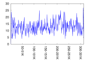
Figure 14: Number of Prominent Facts for Each $1$K Tuples, $\tau$=$10^{3}$

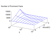
(a) By Number of Bound Dimension Attributes

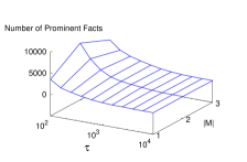
(b) By Dimensionality of Measure Subspaces

Figure 15: Distribution of Prominent Facts, Varying $\tau$

A tuple may be in the contextual skylines of many constraint-measure pairs. For instance, $t_{7}$ in Example 1 belongs to $196$ contextual skylines (of course partly because the table is tiny and most contexts contain only $t_{7}$). Reporting all such facts overwhelms users and makes important facts harder to spot. It is crucial to report truly prominent facts, which should be rare. We measure the prominence of a fact (i.e., a constraint-measure pair $(C,M)$) by $\smash{|\sigma_{C}(R)|\over|\lambda_{M}(\sigma_{C}(R))|}$, the cardinality ratio of all tuples to skyline tuples in the context. Consider two pairs in Example 1:($C_{1}$:month=Feb,$M_{1}$:{points,assists,rebounds}) and ($C_{2}$:team=Celtics$\wedge$opp_team=Nets,$M_{2}$:{assists,rebounds}). The context of $C_{1}$ contains $5$ tuples, among which $t_{2}$ and $t_{7}$ are in the skyline in $M_{1}$. Hence, the prominence of ($C_{1},M_{1}$) is $5/2$. Similarly the prominence of ($C_{2},M_{2}$) is $3/2$. Hence ($C_{1},M_{1}$) is more prominent, because larger ratios indicate rarer events.

For a newly arrived tuple $t$, we rank all situational facts $S^{t}$ pertinent to $t$ in descending order of their prominence. A fact is prominent if its prominence value is the highest among $S^{t}$ and is not below a given threshold $\tau$. (There can be multiple prominent facts pertinent to the arrival of $t$, due to ties in their prominence values.) Consider $t_{7}$ in Example 1. From the $196$ facts in $S^{t_{7}}$, the highest prominence value is $3$. If $\tau$$\leq$$3$, those facts in $S^{t_{7}}$ attaining value $3$ are the prominent facts pertinent to $t_{7}$. Among many such facts, examples are (player=Wesley, {rebounds}) and (month=Feb.$\wedge$team=Celtics,{points}). Note that, based on the definition of the prominence measure and the threshold $\tau$, a context must have at least $\tau$ tuples in order to contribute a prominent fact.

We studied the prominence of situational facts from the NBA dataset, under the parameter setting $d$=$5$, $m$=$7$, $\hat{d}$=$3$, $\hat{m}$=$3$ and $\tau$=$500$. In other words, each prominent fact on a new tuple $t$ is about a contextual skyline that contains $t$ and at most $0.2\%$ of the tuples in the context. Below we show some of the discovered prominent facts. They do not necessarily stand in the real world, since our dataset does not include the complete NBA records from all seasons.

• Lamar Odom had 30 points, 19 rebounds and 11 assists on March 6, 2004. No one before had a better or equal performance in NBA history.

• Allen Iverson had 38 points and 16 assists on April 14, 2004 to become the first player with a 38/16 (points/assists) game in the 2004-2005 season.

• Damon Stoudamire scored 54 points on January 14, 2005. It is the highest score in history made by any Trail Blazers.

Figs.15 and 15 help us further understand the prominent facts from this experiment at the macro-level. Fig.15 shows the number of prominent facts for each 1000 tuples, given threshold $\tau$=$10^{3}$. For instance, there are $11$ prominent facts in total from the $100{,}000^{\text{th}}$ tuple to the $101{,}000^{\text{th}}$ tuple. We observed that the values in Fig.15 mostly oscillate between $5$ and $25$. Consider the number of tuples and the huge number of constraint-measure pairs, these prominent facts are truly selective. One might expect a downward trend in Fig.15. It did not occur due to the constant formulation of new contexts. Each year, a new NBA regular season commences and some new players start to play. Such new values of dimension attributes season and player, coupled with combinations of other dimension attributes, form new contexts. Once a context is populated with enough tuples (at least $\tau$), a newly arrived tuple belonging to the context may trigger a prominent fact.

Fig.15(a) shows the distribution of prominent facts by the number of bound dimension attributes in constraint for varying $\tau$ in $[10^{2},10^{4}]$. Fig.15(b) shows the distribution by the dimensionality of measure subspace. We observed fewer prominent facts with $0$ and $3$ bound attributes (out of $d$=$5$ dimension attributes) than those with $1$ and $2$ bound attributes, and fewer prominent facts in measure subspaces with $1$ and $3$ attributes than those with $2$ attributes. The reasons are: 1) With regard to dimension attributes, if there are no bound attributes in the constraint, the context includes the whole table. Naturally it is more challenging to establish a prominent fact for the whole table. If the constraint has more bound attributes, the corresponding context becomes more specific and contains fewer tuples, which may not be enough to contribute a prominent fact (recall that having one prominent fact entails a context size of no less than $\tau$). Therefore, there are fewer prominent streaks with $3$ bound attributes. 2) With regard to measure attributes, on a single measure, a tuple must have the highest value in order to top other tuples, which does not often happen. There are thus fewer prominent facts in single-attribute subspaces. In a subspace with $3$ attributes, there are also fewer prominent facts, because the contextual skyline contains more tuples, leading to a smaller prominence value that may not beat the threshold $\tau$.

VIII Conclusion

We studied the novel problem of discovering prominent situational facts, which is formalized as finding the constraint-measure pairs that qualify a new tuple as a contextual skyline tuple. We presented algorithms for efficient discovery of prominent facts. We used a simple prominence measure to rank discovered facts. Extensive experiments over two real datasets validated the effectiveness and efficiency of the techniques. This is our first step towards general fact finding for computational journalism. Going forward, we plan to explore several directions, including generalizing the solution for allowing deletion and update of data, narrating facts in natural-language text and reporting facts of other forms (e.g., facts about multiple tuples in a dataset and aggregates over tuples).

IX Acknowledgement

The work of Li is partially supported by NSF Grant IIS-1018865, CCF-1117369, 2011 and 2012 HP Labs Innovation Research Award, and the National Natural Science Foundation of China Grant 61370019. The work of Yang is supported by IIS-0916027 and IIS-1320357. Any opinions, findings, and conclusions or recommendations expressed in this publication are those of the author(s) and do not necessarily reflect the views of the funding agencies.

References

- [1] http://www.newsday.com/sports/columnists/neil-best/hirdt-enjoying-long-run-as-stats-guru-1.3174737. Accessed: Jul. 2013.
- [2] F. Alvanaki, E. Ilieva, S. Michel, and A. Stupar. Interesting event detection through hall of fame rankings. In DBSocial, pages 7–12, 2013.
- [3] J. L. Bentley. Multidimensional binary search trees in database applications. Software Engineering, IEEE Transactions on, (4):333–340, 1979.
- [4] A. Bharadwaj. Automatic Discovery of Significant Events From Databases. Master’s thesis, Universioty of Tesax at Arlington, Dec. 2011.
- [5] S. Börzsönyi, D. Kossmann, and K. Stocker. The skyline operator. In ICDE, pages 421–430, 2001.
- [6] S. Cohen, J. T. Hamilton, and F. Turner. Computational journalism. Commun. ACM, 54(10):66–71, Oct. 2011.
- [7] S. Cohen, C. Li, J. Yang, and C. Yu. Computational journalism: A call to arms to database researchers. In CIDR, pages 148–151, 2011.
- [8] X. Jiang, C. Li, P. Luo, M. Wang, and Y. Yu. Prominent streak discovery in sequence data. In KDD, pages 1280–1288, 2011.
- [9] J. Pei, Y. Yuan, X. Lin, W. Jin, M. Ester, Q. Liu, W. Wang, Y. Tao, J. X. Yu, and Q. Zhang. Towards multidimensional subspace skyline analysis. ACM Trans. Database Syst., 31(4):1335–1381, 2006.
- [10] T. Wu, D. Xin, Q. Mei, and J. Han. Promotion analysis in multi-dimensional space. Proc. VLDB Endow., 2(1):109–120, 2009.
- [11] Y. Wu, P. K. Agarwal, C. Li, J. Yang, and C. Yu. On “one of the few” objects. In KDD, pages 1487–1495, 2012.
- [12] T. Xia and D. Zhang. Refreshing the sky: the compressed skycube with efficient support for frequent updates. In SIGMOD, 2006.
- [13] M. Zhang and R. Alhajj. Skyline queries with constraints: Integrating skyline and traditional query operators. DKE, 69(1):153 – 168, 2010.