A numerical algorithm for fully nonlinear HJB equations:
an approach by control randomization

Abstract

We propose a probabilistic numerical algorithm to solve Backward Stochastic Differential Equations (BSDEs) with nonnegative jumps, a class of BSDEs introduced in [9] for representing fully nonlinear HJB equations. In particular, this allows us to numerically solve stochastic control problems with controlled volatility, possibly degenerate. Our backward scheme, based on least-squares regressions, takes advantage of high-dimensional properties of Monte-Carlo methods, and also provides a parametric estimate in feedback form for the optimal control. A partial analysis of the error of the scheme is provided, as well as numerical tests on the problem of superreplication of option with uncertain volatilities and/or correlations, including a detailed comparison with the numerical results from the alternative scheme proposed in [7].

Key words: Backward stochastic differential equations, control randomization, HJB equation, uncertain volatility, empirical regressions, Monte-Carlo.

MSC Classification: 60H10, 65Cxx, 93E20.

1 Introduction

Consider the following general Hamilton-Jacobi-Bellman (HJB) equation:

$$\frac{\partial v}{\partial t}+\sup_{a\in A}\left\{b\left(x,a\right).D_{x}v+\frac{1}{2}\mathrm{tr}\left(\sigma\sigma^{\top}\left(x,a)\right)D_{x}^{2}v\right)+f\left(x,a,v,\sigma^{\top}\left(x,a\right).D_{x}v\right)\right\} =0\,\,,\,\left(t,x\right)\in\left[0,T\right)\times\mathbb{R}^{d}$$ (1.1)

$$v\left(T,x\right) =g\left(x\right)\,,\,x\in\mathbb{R}^{d}$$

where $A$ is a bounded subset of $\mathbb{R}^{q}$. It is well known that the HJB equation (1.1) is the dynamic programming equation for the following stochastic control problem:

$$v\left(t,x\right) =\sup_{\alpha\in\mathcal{A}}\mathbb{E}^{t,x}\left[\int_{t}^{T}f\left(X_{s}^{\alpha},\alpha_{s}\right)ds+g\left(X_{T}^{\alpha}\right)\right]$$ (1.2)

$$dX_{s}^{\alpha} =b\left(X_{s}^{\alpha},\alpha_{s}\right)ds+\sigma\left(X_{s}^{\alpha},\alpha_{s}\right)dW_{s}$$

Moreover, it is proved in [9] that this HJB equation admits a probabilistic representation by means of a BSDE with nonpositive jumps. We recall below this construction.

Introduce a Poisson random measure $\mu_{A}\left(dt,da\right)$ on $\mathbb{R}_{+}\times A$ with finite intensity measure $\lambda_{A}\left(da\right)dt$ associated to the marked point process $\left(\tau_{i},\zeta_{i}\right)_{i}$, independent of $W$, and consider the pure jump process $\left(I_{t}\right)_{t}$, valued in $A$, defined as follows:

$$I_{t}=\zeta_{i}\,,\,\,\tau_{i}\leq t<\tau_{i+1}\,,$$

and interpreted as a randomization of the control process $\alpha$.

Next, consider the uncontrolled forward regime switching diffusion process

$$dX_{s}=b\left(X_{s},I_{s}\right)ds+\sigma\left(X_{s},I_{s}\right)dW_{s}\,.$$

Observe that the pair process $\left(X,I\right)$ is Markov. Now, consider the following BSDE with jumps w.r.t. the Brownian-Poisson filtration $\mathbb{F}=\mathbb{F}^{W,\mu_{A}}=\left(\mathcal{F}_{t}\right)_{0\leq t\leq T}$.

$$Y_{t}=g\left(X_{T}\right)+\int_{t}^{T}f\left(X_{s},I_{s},Y_{s},Z_{s}\right)ds-\int_{t}^{T}Z_{s}dW_{s}-\int_{t}^{T}\int_{A}U_{s}\left(a\right)\tilde{\mu}_{A}\left(ds,da\right)$$ (1.3)

where $\tilde{\mu}_{A}$ is the compensated measure of $\mu_{A}$.

Finally, we constrain the jump component of the BSDE (1.3) to be nonpositive, i.e.

$$U_{t}\left(a\right)\leq 0,\,\,d\mathbb{P}\otimes dt\otimes\lambda\left(da\right)\,a.e.$$

We denote by $\bar{A}$ $>$ $0$ an upper bound for the compact set $A$ of $\mathbb{R}^{q}$, i.e. $|a|$ $\leq$ $\bar{A}$ for all $a$ $\in$ $A$, and we make the standing assumptions:

1. The functions $b$ and $\sigma$ are Lipschitz: there exists $L_{b,\sigma}$ $>$ $0$ s.t.

   $$|b(x_{1},a_{1})-b(x_{2},a_{2})|+|\sigma(x_{1},a_{1})-\sigma(x_{2},a_{2})| \leq L_{b,\sigma}\big{(}|x_{1}-x_{2}|+|a_{1}-a_{2}|\big{)},$$

   for all $x_{1},x_{2}$ $\in$ $\mathbb{R}^{d}$, $a_{1},a_{2}$ $\in$ $A$.

2. The functions $f$ and $g$ are Lipschitz continuous: there exists $L_{g},L_{f}>0$ s.t.

   $$\left|g\left(x_{1}\right)-g\left(x_{2}\right)\right| \leq L_{g}\left|x_{1}-x_{2}\right|$$

   $$\left|f\left(x_{1},a_{1},y_{1},z_{1}\right)-f\left(x_{2},a_{2},y_{2},z_{2}\right)\right| \leq L_{f}\left(\left|x_{1}-x_{2}\right|+\left|a_{1}-a_{2}\right|+\left|y_{1}-y_{2}\right|+\left|z_{1}-z_{2}\right|\right),$$

   for all $x_{1},x_{2}$ $\in$ $\mathbb{R}^{d}$, $a_{1},a_{2}$ $\in$ $A$.

Under these conditions, we consider the minimal solution $\left(Y,Z,U,K\right)$ of the following constrained BSDE:

$$Y_{t} = g\left(X_{T}\right)+\int_{t}^{T}f\left(X_{s},I_{s},Y_{s},Z_{s}\right)ds-\int_{t}^{T}Z_{s}dW_{s}$$

$$+K_{T}-K_{t}-\int_{t}^{T}\int_{A}U_{s}\left(a\right)\tilde{\mu}_{A}\left(ds,da\right)\,,\,\,0\leq t\leq T\,,\,a.s.$$

subject to the constraint

$$U_{t}\left(a\right)\leq 0\,,\,\,d\mathbb{P}\otimes dt\otimes\lambda\left(da\right)\,a.e.\,\mathrm{on}\,\Omega\times\left[0,T\right]\times A$$ (1.5)

By the Markov property of $\left(X_{t},I_{t}\right)$, there exists a deterministic function $y=y\left(t,x,a\right)$ such that the minimal solution to (1)-(1.5) satisfies $Y_{t}=y\left(t,X_{t},I_{t}\right)$, $0\leq t\leq T$.

Theorem 1.1.

[9] $y=y\left(t,x,a\right)$ does not depend on $a$: $y=y\left(t,x\right)$, and is a viscosity solution of the HJB equation (1.1):

$$\frac{\partial y}{\partial t}+\sup_{a\in A}\left\{b\left(x,a\right).D_{x}y\left(t,x\right)+\frac{1}{2}\mathrm{tr}\left(\sigma\sigma^{\top}\!\!\left(x,a\right)D_{x}^{2}v\left(t,x\right)\right)+f\left(x,a,y,\sigma^{\top}\!\!\left(x,a\right)D_{x}y\right)\right\} =0$$

$$\left(t,x\right)\in\left[0,T\right)\times\mathbb{R}^{d}\hskip 256.0748ptv\left(T,x\right) =g\left(x\right),x\!\in\!\mathbb{R}^{d}$$

Now, the aim of this paper is to provide a numerical scheme for computing an approximation of the solution of the constrained BSDE (1)-(1.5). In light of Theorem 1.1, this will provide an approximation of the solution of the general HJB equation (1.1), which encompasses stochastic control problems such as the one described in equation (1.2), ie. problems where both the drift and the volatility of the underlying diffusion can be controlled, including degenerate diffusion coefficient.

The outline of the subsequent sections is the following.

First, Section 2 describes our scheme. We start from a time-discretization of the problem, proposed in [8], which gives rise to a backward scheme involving the simulation of the forward regime switching process $(X,I)$, hence taking advantage of high-dimensional properties of Monte-Carlo methods. The final step towards an implementable scheme is to approximate the conditional expectations that arise from this scheme. Here we use empirical least-squares regression, as this method provides a parametric estimate in feedback form of the optimal control. A partial analysis of the impact of this approximation is provided, and the remaining obstacles towards a full analysis are highlighted.

Then, Section 3 is devoted to numerical tests of the scheme on various examples. The major application that takes advantage of the possibilities of our scheme is the problem of pricing and hedging contingent claims under uncertain volatility and (for multi-dimensional claims) correlation. Therefore most of this section is devoted to this specific application. To our knowledge, the only other Monte Carlo scheme for HJB equations that can handle continuous controls as well as controlled volatility is described in [7], where they make use of another generalization of BSDEs, namely second-order BSDEs. Therefore we compare the performance of our scheme to the results provided in their paper.

Finally, Section 4 concludes the paper.

2 Regression scheme

Define a deterministic time grid $\pi$:=$\left\{0=t_{0}<\ldots<t_{N}=T\right\}$ for the interval $[0,T]$, with mesh $\left|\pi\right|:=\max_{0\leq i<N}\Delta_{i}$ where $\Delta_{i}:=t_{i+1}-t_{i}$. Denote by $\mathbb{E}_{i}\left[.\right]:=\mathbb{E}\left[.\left|\mathcal{F}_{t_{i}}\right.\right]=\mathbb{E}\left[.\left|X_{i},I_{i}\right.\right]$. The discretization of the constrained BSDE (1)-(1.5) can be written as follows:

$$\begin{cases}Y_{N}&=g\left(X_{N}\right)\\ \Delta_{i}\mathcal{Z}_{i}&=\mathbb{E}_{i}\left[Y_{i+1}\Delta W_{i}^{\top}\right]\\ \mathcal{Y}_{i}&=\mathbb{E}_{i}\left[Y_{i+1}+f\left(X_{i},I_{i},Y_{i+1},\mathcal{Z}_{i}\right)\Delta_{i}\right]\\ Y_{i}&=\underset{a\in A}{\mathrm{ess\,sup\,}}\mathbb{E}_{i,a}\left[\mathcal{Y}_{i}\right]\end{cases}$$ (2.1)

where $\mathbb{E}_{i,a}\left[.\right]:=\mathbb{E}\left[.\left|X_{i},I_{i},I_{i}=a\right.\right]=\mathbb{E}\left[.\left|X_{i},I_{i}=a\right.\right]$.

First, remark that, from the Markov property of $\left(X_{i},I_{i}\right)_{1\leq i\leq N}$, there exist deterministic functions $\tilde{y}_{i}$ and $\tilde{z}_{i}$ such that $\left(\mathcal{Y}_{i},\mathcal{Z}_{i}\right)=\left(\tilde{y}_{i}\left(X_{i},I_{i}\right),\tilde{z}_{i}\left(X_{i},I_{i}\right)\right)$. Hence $\mathcal{Y}_{i}$ and $\mathcal{Z}_{i}$ can be seen as intermediate quantities towards the discrete-time approximation of the BSDE (1)-(1.5) $\left(Y_{i},Z_{i}\right)=\left(y_{i}\left(X_{i}\right),z_{i}\left(X_{i}\right)\right)$ , which do not depend on $I_{i}$.

Formally, the jump constraint (1.5) states that $\tilde{y}_{i}\left(X_{i},a\right)-y_{i}\left(X_{i}\right)=U_{t}\left(a\right)\leq 0$ a.s., meaning that the minimal solution satisfies $Y_{i}=y_{i}\left(X_{i}\right)=\underset{a\in A}{\mathrm{ess\,sup\,}}\tilde{y}_{i}\left(X_{i},a\right)=\underset{a\in A}{\mathrm{ess\,sup\,}}\mathbb{E}_{i,a}\left[\mathcal{Y}_{i}\right]$.

Moreover, one can extract $Z_{i}$ from the scheme if needed. Indeed, denoting $a^{*}=\arg\underset{a\in A}{\mathrm{ess\,sup\,}}\mathbb{E}_{i,a}\left[\mathcal{Y}_{i}\right]$, i.e. $Y_{i}=\mathbb{E}_{i,a^{*}}\left[\mathcal{Y}_{i}\right]$, then $Z_{i}=z_{i}\left(X_{i}\right)=\tilde{z}_{i}\left(X_{i},a^{*}\right)$.

Finally remark that the numerical scheme (2.1) is explicit, as we choose to define $\mathcal{Y}_{i}$ as a function of $Y_{i+1}$ and not of $Y_{i}$.

The convergence of the solution of the discretized scheme (2.1) towards the solution of the constrained BSDE (1)-(1.5) is thoroughly examined in [8]. In this paper, we start from the discrete version (2.1) and derive an implementable scheme from it.

Indeed, the discrete scheme (2.1) is in general not readily implementable because it involves conditional expectations that cannot be computed explicitly. It is thus necessary in practice to approximate these conditional expectations. Here we follow the empirical regression approach ([10, 3, 6, 18, 1]). In our context, apart from being easy to implement, the strong advantage of this choice is that, unlike other standard methods, it provides as a by-product a parametric feedback estimate $\hat{\alpha}\left(t,X_{t}\right)$ for the optimal control.

The idea is to replace the conditional expectations from (2.1) by empirical regressions. This section is devoted to the analysis of the error generated by this replacement.

2.1 Localizations

The first step is to localize the discrete BSDE (2.1), i.e. to truncate it so that it admits a.s. deterministic bounds. Introduce $R_{X}\in\mathbb{R}_{+}^{d}$ and $R_{w}\in\mathbb{R}_{+}$ and define the following truncations of $X_{i}$ and $\Delta W_{i}$:

$$\left[X_{i}\right]_{X} :=-R_{X}\vee X_{i}\wedge R_{X}=\left\{-R_{1,X}\vee X_{1,i}\wedge R_{1,X},\ldots,-R_{d,X}\vee X_{d,i}\wedge R_{d,X}\right\}^{\top}$$ (2.2)

$$\left[\Delta W_{i}\right]_{w} :=-R_{w}\sqrt{\Delta_{i}}\vee\Delta W_{i}\wedge R_{w}\sqrt{\Delta_{i}}=\left\{-R_{w}\sqrt{\Delta_{i}}\vee\Delta W_{1,i}\wedge R_{w}\sqrt{\Delta_{i}},\ldots,-R_{w}\sqrt{\Delta_{i}}\vee\Delta W_{q,i}\wedge R_{w}\sqrt{\Delta_{i}}\right\}^{\top}$$ (2.3)

Define $R=\left\{R_{X},R_{w}\right\}$ and define the localized version of the discrete BSDE (2.1), using the truncations (2.2) and (2.3).

$$\begin{cases}Y_{N}^{R}&=g\left(\left[X_{N}\right]_{X}\right)\\ \Delta_{i}\mathcal{Z}_{i}^{R}&=\mathbb{E}_{i}\left[Y_{i+1}^{R}\left[\Delta W_{i}^{\top}\right]_{w}\right]\\ \mathcal{Y}_{i}^{R}&=\mathbb{E}_{i}\left[Y_{i+1}^{R}+f\left(\left[X_{i}\right]_{X},I_{i},Y_{i+1}^{R},\mathcal{Z}_{i}^{R}\right)\Delta_{i}\right]\\ Y_{i}^{R}&=\underset{a\in A}{\mathrm{ess\,sup\,}}\mathbb{E}_{i,a}\left[\mathcal{Y}_{i}^{R}\right]\end{cases}$$ (2.4)

First, we check that this localized BSDE does admit a.s. bounds.

Lemma 2.1.

[almost sure bounds] For every $R=\left\{R_{X},R_{w}\right\}\in\left[0,\infty\right)^{d}\times\left[0,\infty\right]$ and every $1\leq i\leq N$, the following uniform bounds hold a.s.:

$$\left|\mathcal{Y}_{i}^{R}\right|,\left|Y_{i}^{R}\right| \leq C_{y}=C_{y}\left(R_{X}\right):=e^{\frac{C}{2}T}\sqrt{C_{g}^{2}\left(R_{X}\right)+\frac{e^{C\left|\pi\right|}}{L_{f}^{2}}C_{f}^{2}\left(R_{X}\right)}$$

$$\left|\mathcal{Z}_{i}^{R}\right|,\left|Z_{i}^{R}\right| \leq C_{z}=C_{y}\left(R_{X}\right):=\frac{\sqrt{q}}{\sqrt{\Delta_{i}}}C_{y}$$

where $C:=3L_{f}^{2}\left(q+\left|\pi\right|\right)+\frac{1}{q}$, $C_{g}\left(R_{X}\right):=\max_{-R_{X}\leq x\leq R_{X}}\left|g\left(x\right)\right|$ and $C_{f}\left(R_{X}\right):=L_{f}\left(\left|R_{X}\right|+\left|\bar{A}\right|\right)+f\left(0,0,0,0\right)$

Proof.

First, as $g$ is continuous, there exists $C_{g}=C_{g}\left(R_{X}\right)>0$ such that for all $-R_{X}\leq x\leq R_{X}$, $\left|g\left(x\right)\right|\leq C_{g}\left(R_{X}\right)$. Hence

$$\left(Y_{N}^{R}\right)^{2}=g^{2}\left(\left[X_{N}\right]_{X}\right)\leq C_{g}^{2}\left(R_{X}\right)$$ (2.5)

Next,

$$\Delta_{i}\mathcal{Z}_{i}^{R}=\mathbb{E}_{i}\left[Y_{i+1}^{R}\left[\Delta W_{i}\right]_{w}\right]=\mathbb{E}_{i}\left[\left(Y_{i+1}^{R}-\mathbb{E}_{i}\left[Y_{i+1}^{R}\right]\right)\left[\Delta W_{i}\right]_{w}\right]$$

Thus, using the Cauchy-Schwarz inequality and dividing by $\Delta_{i}$:

$$\Delta_{i}\left(\mathcal{Z}_{i}^{R}\right)^{2}\leq q\left(\mathbb{E}_{i}\left[\left(Y_{i+1}^{R}\right)^{2}\right]-\mathbb{E}_{i}\left[Y_{i+1}^{R}\right]^{2}\right)$$

Now, using Young’s inequality $\left(a+b\right)^{2}\leq\left(1+\gamma\Delta_{i}\right)a^{2}+\left(1+\frac{1}{\gamma\Delta_{i}}\right)b^{2}$ with $\gamma>0$:

$$\left(\mathcal{Y}_{i}^{R}\right)^{2}\leq\left(1+\gamma\Delta_{i}\right)\mathbb{E}_{i}\left[Y_{i+1}^{R}\right]^{2}+\left(1+\frac{1}{\gamma\Delta_{i}}\right)\Delta_{i}^{2}\mathbb{E}_{i}\left[f^{2}\left(\left[X_{i}\right]_{X},I_{i},Y_{i+1}^{R},\mathcal{Z}_{i}^{R}\right)\right]$$

Remark that

$$\left|f\left(\left[X_{i}\right]_{X},I_{i},Y_{i+1}^{R},\mathcal{Z}_{i}^{R}\right)\right| \leq \left|f\left(\left[X_{i}\right]_{X},I_{i},Y_{i+1}^{R},\mathcal{Z}_{i}^{R}\right)-f\left(0,0,0,0\right)\right|+\left|f\left(0,0,0,0\right)\right|$$

$$\leq L_{f}\left(\left|\left[X_{i}\right]_{X}\right|+\left|I_{i}\right|+\left|Y_{i+1}^{R}\right|+\left|\mathcal{Z}_{i}^{R}\right|\right)+\left|f\left(0,0,0,0\right)\right|$$

$$\leq C_{f}\left(R_{X}\right)+L_{f}\left(\left|Y_{i+1}^{R}\right|+\left|\mathcal{Z}_{i}^{R}\right|\right)$$

where $C_{f}\left(R_{X}\right):=L_{f}\left(\left|R_{X}\right|+\left|\bar{A}\right|\right)+\left|f\left(0,0,0,0\right)\right|$. Hence

$$\left(\mathcal{Y}_{i}^{R}\right)^{2} \leq \left(1+\gamma\Delta_{i}\right)\mathbb{E}_{i}\left[Y_{i+1}^{R}\right]^{2}+3\left(\Delta_{i}+\frac{1}{\gamma}\right)\Delta_{i}\left(C_{f}^{2}\left(R_{X}\right)+L_{f}^{2}\mathbb{E}_{i}\left[\left(Y_{i+1}^{R}\right)^{2}\right]+L_{f}^{2}\mathbb{E}_{i}\left[\left|\mathcal{Z}_{i}^{R}\right|\right]\right)$$

$$\leq \left(\Delta_{i}+\frac{1}{\gamma}\right)\left(\mathbb{E}_{i}\left[Y_{i+1}^{R}\right]^{2}\left(\gamma-3qL_{f}^{2}\right)+\mathbb{E}_{i}\left[\left(Y_{i+1}^{R}\right)^{2}\right]3L_{f}^{2}\left(\Delta_{i}-q\right)+3C_{f}^{2}\left(R_{X}\right)\Delta_{i}\right)$$

Thus, for every $\gamma\geq 3qL_{f}^{2}$, one can group together the terms involving $\mathbb{E}_{i}\left[Y_{i+1}^{R}\right]^{2}$ and $\mathbb{E}_{i}\left[\left(Y_{i+1}^{R}\right)^{2}\right]$ using Jensen’s inequality:

$$\left(\mathcal{Y}_{i}^{R}\right)^{2} \leq \left(1+\theta\left(3,\gamma\right)\Delta_{i}\right)\mathbb{E}_{i}\left[\left(Y_{i+1}^{R}\right)^{2}\right]+3\left(\left|\pi\right|+\frac{1}{\gamma}\right)C_{f}^{2}\left(R_{X}\right)\Delta_{i}$$

where $\theta\left(c,\gamma\right):=\gamma+cL_{f}^{2}\left(\left|\pi\right|+\frac{1}{\gamma}\right)$. Finally:

$$\left(Y_{i}^{R}\right)^{2}\leq\underset{a\in A}{\mathrm{ess\,sup\,}}\mathbb{E}_{i,a}\left[\left(Y_{i+1}^{R}\right)^{2}\right]\left(1+\theta\left(3,\gamma\right)\Delta_{i}\right)+3\left(\left|\pi\right|+\frac{1}{\gamma}\right)C_{f}^{2}\left(R_{X}\right)\Delta_{i}$$ (2.6)

Using equations (2.5) and (2.6), one obtains by induction that:

$$\left(Y_{i}^{R}\right)^{2}\leq\Gamma_{i}^{N-1}\left(3,\gamma\right)C_{g}^{2}\left(R_{X}\right)+3\left(\left|\pi\right|+\frac{1}{\gamma}\right)C_{f}^{2}\left(R_{X}\right)\sum_{k=i}^{N-1}\Gamma_{i}^{k}\left(3,\gamma\right)\Delta_{k}$$ (2.7)

where $\Gamma_{i}^{j}\left(c,\gamma\right):=\Pi_{k=i}^{j}\left(1+\theta\left(c,\gamma\right)\Delta_{k}\right)$. Finally remark that $\forall c,\gamma>0$

$$\ln\left(\Gamma_{i}^{j}\left(c,\gamma\right)\right)=\sum_{k=i}^{j}\ln\left(1+\theta\left(c,\gamma\right)\Delta_{k}\right)\leq\sum_{k=i}^{j}\theta\left(c,\gamma\right)\Delta_{k}=\theta\left(c,\gamma\right)\left(t_{j+1}-t_{i}\right)$$

Thus

$$\Gamma_{i}^{j}\left(c,\gamma\right)\leq\exp\left(\theta\left(c,\gamma\right)\left(t_{j+1}-t_{i}\right)\right)$$ (2.8)

And

$$\sum_{k=i}^{N-1}\Gamma_{i}^{k}\left(c,\gamma\right)\Delta_{k} \leq \sum_{k=i}^{N-1}e^{\theta\left(c,\gamma\right)\left(t_{j+1}-t_{i}\right)}\Delta_{k}\leq e^{\theta\left(c,\gamma\right)\left|\pi\right|}\sum_{k=i}^{N-1}e^{\theta\left(c,\gamma\right)\left(t_{j}-t_{i}\right)}\Delta_{k}$$ (2.9)

$$\leq e^{\theta\left(c,\gamma\right)\left|\pi\right|}\int_{t_{i}}^{t_{N}}e^{\theta\left(c,\gamma\right)\left(t-t_{i}\right)}dt=\frac{e^{\theta\left(c,\gamma\right)\left|\pi\right|}}{\theta\left(c,\gamma\right)}\left(e^{\theta\left(c,\gamma\right)\left(t_{N}-t_{i}\right)}-1\right)$$

Finally, combine equations (2.7), (2.8) and (2.9) with $c=3$ and $\gamma\geq 3qL_{f}^{2}$ to obtain the following a.s. bound for $Y_{i}^{R}$ :

$$\left(Y_{i}^{R}\right)^{2} \leq e^{\theta\left(3,\gamma\right)\left(t_{N}-t_{i}\right)}C_{g}^{2}\left(R_{X}\right)+3\left(\left|\pi\right|+\frac{1}{\gamma}\right)C_{f}^{2}\left(R_{X}\right)\frac{e^{\theta\left(3,\gamma\right)\left|\pi\right|}}{\theta\left(3,\gamma\right)}\left(e^{\theta\left(3,\gamma\right)\left(t_{N}-t_{i}\right)}-1\right)$$

$$\leq e^{\theta\left(3,\gamma\right)T}\left\{C_{g}^{2}\left(R_{X}\right)+3\frac{e^{\theta\left(3,\gamma\right)\left|\pi\right|}}{\theta\left(3,\gamma\right)}\left(\left|\pi\right|+\frac{1}{\gamma}\right)C_{f}^{2}\left(R_{X}\right)\right\}$$

In particular, for $c=3$ and $\gamma=3qL_{f}^{2}$:

$$\left(Y_{i}^{R}\right)^{2} \leq e^{CT}\left\{C_{g}^{2}\left(R_{X}\right)+\frac{e^{C\left|\pi\right|}}{L_{f}^{2}}C_{f}^{2}\left(R_{X}\right)\right\}=:C_{y}^{2}$$

where $C:=3L_{f}^{2}\left(q+\left|\pi\right|\right)+\frac{1}{q}$. The same inequality holds for $\left(\mathcal{Y}_{i}^{R}\right)^{2}$. For $\mathcal{Z}_{i}^{R}$, use the Cauchy-Schwarz inequality to obtain:

$$\left(\mathcal{Z}_{i}^{R}\right)^{2}\leq\frac{q}{\Delta_{i}}\mathbb{E}_{i}\left[\left(Y_{i+1}^{R}\right)^{2}\right]\leq\frac{q}{\Delta_{i}}C_{y}^{2}=:C_{z}^{2}$$

and the same inequality holds for $\left(Z_{i}^{R}\right)^{2}$.∎

Lemma 2.2.

For $R>0$, define $\mathcal{T}_{R}=\mathbb{E}\left[\left(\mathcal{N}-\left(-R\right)\vee\mathcal{N}\wedge R\right)^{2}\right]$ where $\mathcal{N}$ is a Gaussian random variable with mean $0$ and variance $1$. Then:

$$\mathcal{T}_{R}\leq\sqrt{\frac{2}{\pi}}\frac{1}{R}e^{-\frac{R^{2}}{2}}$$

Proof.

Developing the square yields

$$\mathcal{T}_{R}=2R^{2}\mathbb{P}\left(\mathcal{N}>R\right)-4R\mathbb{E}\left[\mathcal{N}\mathbf{1}\left\{\mathcal{N}>R\right\}\right]+2\mathbb{E}\left[\mathcal{N}^{2}\mathbf{1}\left\{\mathcal{N}>R\right\}\right]$$

Then the two expectations can be explicited as follows

$$\mathbb{E}\left[\mathcal{N}\mathbf{1}\left\{\mathcal{N}>R\right\}\right] = \frac{e^{-\frac{R^{2}}{2}}}{\sqrt{2\pi}}$$

$$\mathbb{E}\left[\mathcal{N}^{2}\mathbf{1}\left\{\mathcal{N}>R\right\}\right] = \frac{R}{\sqrt{2\pi}}e^{-\frac{R^{2}}{2}}+\mathbb{P}\left(\mathcal{N}>R\right)$$

Finally, the use of Mill’s ratio inequality $\mathbb{P}\left(\mathcal{N}>R\right)<\frac{1}{R}\frac{e^{-\frac{R^{2}}{2}}}{\sqrt{2\pi}}$ concludes the proof. ∎

Then, we can estimate bounds between the BSDEs (2.1) and (2.4).

Proposition 2.1.

The following bounds hold:

$$\left(Y_{i}-Y_{i}^{R}\right)^{2} \leq e^{CT}\left\{L_{g}\left(\left|\Delta X_{N}\right|^{2}\right)^{*}+C\sum_{k=i}^{N-1}\Delta_{k}\left(\left|\Delta X_{k}\right|^{2}\right)^{*}+2qCTC_{y}^{2}\mathcal{T}_{R_{w}}\right\}$$

where $C:=3L_{f}^{2}\left(2q+\left|\pi\right|\right)+\frac{1}{2q}$, and $\left(\left|\Delta X_{k}\right|^{2}\right)^{*}$, $k\geq i$, is the solution of the following linear constrained BSDE:

$$\begin{cases}Y_{k}&=\left(X_{k}-\left[X_{k}\right]_{X}\right)^{2}\\ Y_{j}&=\underset{a\in A}{\mathrm{ess\,sup\,}}\mathbb{E}_{j,a}\left[Y_{j+1}\right]\,,\,\,j=k-1,\ldots,i\end{cases}$$

Proof.

Define $\Delta X_{i}=X_{i}-\left[X_{i}\right]_{X}$, $\Delta Y_{i}=Y_{i}-Y_{i}^{R}$, $\Delta\mathcal{Y}_{i}=\mathcal{Y}_{i}-\mathcal{Y}_{i}^{R}$, $\Delta Z_{i}=Z_{i}-Z_{i}^{R}$ and $\Delta\mathcal{Z}_{i}=\mathcal{Z}_{i}-\mathcal{Z}_{i}^{R}$. First

$$\left|\Delta Y_{N}\right|=\left|g\left(X_{N}\right)-g\left(\left[X_{N}\right]_{X}\right)\right|\leq L_{g}\left|\Delta X_{N}^{p}\right|$$

Then

$$\Delta_{i}\Delta\mathcal{Z}_{i} = \mathbb{E}_{i}\left[Y_{i+1}\Delta W_{i}^{\top}-Y_{i+1}^{R}\left[\Delta W_{i}^{\top}\right]_{w}\right]$$

$$= \mathbb{E}_{i}\left[\Delta Y_{i+1}\Delta W_{i}^{\top}+Y_{i+1}^{R}\left\{\Delta W_{i}-\left[\Delta W_{i}\right]_{w}\right\}^{\top}\right]$$

$$\mathbb{E}_{i}\left[\left(\Delta Y_{i+1}-\mathbb{E}_{i}\left[\Delta Y_{i+1}\right]\right)\Delta W_{i}^{\top}\right]+\mathbb{E}_{i}\left[Y_{i+1}^{R}\left\{\Delta W_{i}-\left[\Delta W_{i}\right]_{w}\right\}^{\top}\right]$$

Hence

$$\Delta_{i}\left(\Delta\mathcal{Z}_{i}\right)^{2}\leq 2q\left(\mathbb{E}_{i}\left[\left(\Delta Y_{i+1}\right)^{2}\right]-\mathbb{E}_{i}\left[\Delta Y_{i+1}\right]^{2}\right)+2qC_{y}^{2}\mathcal{T}_{R_{w}}$$

Then

$$\Delta\mathcal{Y}_{i}=\mathbb{E}_{i}\left[\Delta Y_{i+1}+\left\{f\left(X_{i},I_{i},Y_{i+1},\mathcal{Z}_{i}\right)-f\left(\left[X_{i}\right]_{X},I_{i},Y_{i+1}^{R},\mathcal{Z}_{i}^{R}\right)\right\}\Delta_{i}\right]$$

Using Jensen’s inequality and Young’s inequality with parameter $\gamma\Delta_{i}$, $\gamma>0$:

$$\left(\Delta\mathcal{Y}_{i}\right)^{2} \leq \left(1+\gamma\Delta_{i}\right)\mathbb{E}_{i}\left[\Delta Y_{i+1}\right]^{2}+\left(1+\frac{1}{\gamma\Delta_{i}}\right)\Delta_{i}^{2}3L_{f}^{2}\mathbb{E}_{i}\left[\left(\Delta X_{i}\right)^{2}+\left(\Delta Y_{i+1}\right)^{2}+\left(\Delta\mathcal{Z}_{i}\right)^{2}\right]$$

$$\leq \mathbb{E}_{i}\left[\Delta Y_{i+1}\right]^{2}\left(\Delta_{i}+\frac{1}{\gamma}\right)\left(\gamma-6qL_{f}^{2}\right)+\mathbb{E}_{i}\left[\left(\Delta Y_{i+1}\right)^{2}\right]\left(\Delta_{i}+\frac{1}{\gamma}\right)3L_{f}^{2}\left(\Delta_{i}+2q\right)$$

$$+\left(\Delta_{i}+\frac{1}{\gamma}\right)\Delta_{i}3L_{f}^{2}\left\{\left(\Delta X_{i}\right)^{2}+2qC_{y}^{2}\mathcal{T}_{R_{w}}\right\}$$

Now, for any $\gamma\geq 6qL_{f}^{2}$, one can group together the terms in $\mathbb{E}_{i}\left[\Delta Y_{i+1}\right]^{2}$ and $\mathbb{E}_{i}\left[\left(\Delta Y_{i+1}\right)^{2}\right]$ using Jensen’s inequality:

$$\left(\Delta\mathcal{Y}_{i}\right)^{2}\leq\mathbb{E}_{i}\left[\left(\Delta Y_{i+1}\right)^{2}\right]\left\{1+\theta\left(3,\gamma\right)\Delta_{i}\right\}+3L_{f}^{2}\left(\left|\pi\right|+\frac{1}{\gamma}\right)\Delta_{i}\left\{\left(\Delta X_{i}\right)^{2}+2qC_{y}^{2}\mathcal{T}_{R_{w}}\right\}$$

where, as in Lemma 2.1, $\theta\left(c,\gamma\right):=\gamma+cL_{f}^{2}\left(\left|\pi\right|+\frac{1}{\gamma}\right)$. Hence, using that for any random variables $\Theta$ and $\Theta^{\prime}$,

$$\left(\underset{a\in A}{\mathrm{ess\,sup\,}}\mathbb{E}_{i,a}\left[\Theta\right]-\underset{a\in A}{\mathrm{ess\,sup\,}}\mathbb{E}_{i,a}\left[\Theta^{\prime}\right]\right)^{2}\leq\underset{a\in A}{\mathrm{ess\,sup\,}}\mathbb{E}_{i,a}\left[\left(\Theta-\Theta^{\prime}\right)^{2}\right]\,,$$

the following holds:

$$\left(\Delta Y_{i}\right)^{2}\leq\left\{1+\theta\left(3,\gamma\right)\Delta_{i}\right\}\underset{a\in A}{\mathrm{ess\,sup\,}}\mathbb{E}_{i,a}\left[\left(\Delta Y_{i+1}\right)^{2}\right]+3L_{f}^{2}\left(\left|\pi\right|+\frac{1}{\gamma}\right)\Delta_{i}\left\{\left(\Delta X_{i}\right)^{2}+2qC_{y}^{2}\mathcal{T}_{R_{w}}\right\}$$

By induction

$$\left(\Delta Y_{i}\right)^{2} \leq L_{g}\Gamma_{i}^{N-1}\left(3,\gamma\right)\left(\left|\Delta X_{N}\right|^{2}\right)^{*}$$

$$+3L_{f}^{2}\left(\left|\pi\right|+\frac{1}{\gamma}\right)\sum_{k=i}^{N-1}\Delta_{k}\Gamma_{i}^{k}\left(3,\gamma\right)\left\{\left(\left|\Delta X_{k}\right|^{2}\right)^{*}+2qC_{y}^{2}\mathcal{T}_{R_{w}}\right\}$$

where, as in Lemma 2.1, $\Gamma_{i}^{j}\left(c,\gamma\right):=\Pi_{k=i}^{j}\left(1+\theta\left(c,\gamma\right)\Delta_{k}\right)\leq\exp\left(\theta\left(c,\gamma\right)\left(t_{j+1}-t_{i}\right)\right)$ . Finally, take $\gamma=6qL_{f}^{2}$ to obtain the desired bound. ∎

2.2 Projections

In its current form, the scheme (2.4) is not readily implementable, because its conditional expectations cannot be computed in general. Therefore, there is a need to approximate these conditional expectations. For handiness and efficiency, we choose, in the spirit of [10] and [6], to approximate them by empirical least-squares regression.

First, we will study the impact of the replacement of the conditional expectations by theoretical least-squares regressions. We will see that the resulting scheme is not easy to analyze. Therefore, we will study a stronger version of it, and discuss their practical differences. As it is already a daunting task for standard BSDEs (cf. [10]), and in view of the difficulties already raised at theoretical regression level, we leave the study of the final replacement of these regressions by their empirical counterparts for further research.

Hence, for each $i\in\left\{0,\ldots,N-1\right\}$, consider $\mathcal{S}_{i}^{Y}$ and $\mathcal{S}_{i}^{Z}=\left\{\mathcal{S}_{i}^{Z,1},\ldots,\mathcal{S}_{i}^{Z,q}\right\}$ that are non-empty closed convex subsets of $\mathbf{L}_{2}\left(\mathcal{F}_{t_{i}},\mathbb{P}\right)$, as well as the corresponding projection operators $\mathcal{P}_{i}^{Y}$ and $\mathcal{P}_{i}^{Z}=\left\{\mathcal{P}_{i}^{Z,1},\ldots,\mathcal{P}_{i}^{Z,q}\right\}$. Using the above projection operators in lieu of the conditional expectations in (2.4), we obtain the following approximation scheme:

$$\begin{cases}\tilde{Y}_{N}^{R}&=g\left(\left[X_{N}\right]_{X}\right)\\ \Delta_{i}\tilde{\mathcal{Z}}_{i}^{R}&=\left[\mathcal{P}_{i}^{Z}\left(\tilde{Y}_{i+1}^{R}\left[\Delta W_{i}^{\top}\right]_{w}\right)\right]_{i,z}\\ \tilde{\mathcal{Y}}_{i}^{R}&=\left[\mathcal{P}_{i}^{Y}\left(\tilde{Y}_{i+1}^{R}+f\left(\left[X_{i}\right]_{X},I_{i},\tilde{Y}_{i+1}^{R},\tilde{\mathcal{Z}}_{i}^{R}\right)\Delta_{i}\right)\right]_{y}\\ \tilde{Y}_{i}^{R}&=\underset{a\in A}{\mathrm{ess\,sup\,}}\mathbb{E}_{i,a}\left[\tilde{\mathcal{Y}}_{i}^{R}\right]\end{cases}$$ (2.10)

where $\left[.\right]_{i,z}:=-\Delta_{i}C_{z}\wedge.\vee\Delta_{i}C_{z}$ and $\left[.\right]_{y}:=-C_{y}\wedge.\vee C_{y}$ are truncation operators that ensure that the a.s. upper bounds for $\left(Y^{R},Z^{R}\right)$ from Lemma 2.1 will also hold for $\left(\tilde{Y}^{R},\tilde{Z}^{R}\right)$.

To be more specific, choose the subsets $\mathcal{S}_{i}^{Y}$ and $\mathcal{S}_{i}^{Z}$ as follows:

$$\mathcal{S}_{i}^{Y} =\left\{\lambda.p_{i}^{Y}\left(X_{i},I_{i}\right)\,;\,\lambda\in\mathbb{R}^{B_{i}^{Y}}\right\}$$

$$\mathcal{S}_{i}^{Z,k} =\left\{\lambda.p_{i}^{Z,k}\left(X_{i},I_{i}\right)\,;\,\lambda\in\mathbb{R}^{B_{i}^{Z,k}}\right\}\,,\,k=1,\ldots,q$$

where $p_{i}^{Y}=\left(p_{i,1}^{Y},\ldots,p_{i,B_{i}^{Y}}^{Y}\right)^{\top}$, $B_{i}^{Y}\geq 1$, and $p_{i}^{Z,k}=\left(p_{i,1}^{Z,k},\ldots,p_{i,B_{i}^{Z,k}}^{,Z,k}\right)^{\top}$, $B_{i}^{Z,k}\geq 1$, are predefined sets of deterministic functions from $\mathbb{R}^{d}\times\mathbb{R}^{q}$ into $\mathbb{R}$. Hence, for any random variable $U$ in $\mathbf{L}_{2}\left(\mathcal{F}_{T},\mathbb{P}\right)$, $\mathcal{P}_{i}^{Y}\left(U\right)$ is defined as follows:

$$\hat{\lambda}_{i}^{Y}\left(U\right) :=\arg\inf_{\lambda\in\mathbb{R}^{B_{i}^{Y}}}\mathbb{E}\left[\left(\lambda.p_{i}^{Y}\left(X_{i},I_{i}\right)-U\right)^{2}\right]$$ (2.11)

$$\mathcal{P}_{i}^{Y}\left(U\right) :=\hat{\lambda}_{i}^{Y}\left(U\right).p_{i}^{Y}\left(X_{i},I_{i}\right)$$

and $\mathcal{P}_{i}^{Z}\left(U\right)$ is defined in a similar manner. With these notations, the scheme (2.10) can be explicited further as follows:

$$\begin{cases}\tilde{Y}_{N}^{R}&=g\left(\left[X_{N}\right]_{X}\right)\\ \Delta_{i}\tilde{\mathcal{Z}}_{i}^{R}&=\left[\hat{\lambda}_{i}^{Z}\left(\tilde{Y}_{i+1}^{R}\left[\Delta W_{i}^{\top}\right]_{w}\right).p_{i}^{Z}\left(X_{i},I_{i}\right)\right]_{i,z}\\ \tilde{Y}_{i}^{R}&=\underset{a\in\mathcal{A}_{i}}{\mathrm{ess\,sup\,}}\left[\hat{\lambda}_{i}^{Y}\left(\tilde{Y}_{i+1}^{R}+f\left(\left[X_{i}\right]_{X},I_{i},\tilde{Y}_{i+1}^{R},\tilde{\mathcal{Z}}_{i}^{R}\right)\Delta_{i}\right).p_{i}^{Y}\left(X_{i},a\right)\right]_{y}\,,\end{cases}$$ (2.12)

where $\mathcal{A}_{i}$ is the set of $\sigma\left(X_{i}\right)$-measurable random variables taking values in $A$. Now, we would like to analyze the error between $\left(Y^{R},Z^{R}\right)$ and $\left(\tilde{Y}^{R},\tilde{Z}^{R}\right)$. Unfortunately, in spite of the simplicity of the scheme (2.12), this analysis is made strenuous by the fact that $\tilde{Y}_{i}^{R}$ is not itself a projection, as it combines regression coefficients computed using the random variable $I_{i}$ and regression functions valued at another random variable $a$. This prevents the analysis from taking advantage of standard tools to deal with least-squares regressions. For comparison, consider the following alternative scheme:

$$\begin{cases}\hat{Y}_{N}^{R}&=g\left(\left[X_{N}\right]_{X}\right)\\ \Delta_{i}\hat{\mathcal{Z}}_{i,a}^{R}&=\left[\hat{\lambda}_{i,a}^{Z}\left(\hat{Y}_{i+1}^{R}\left[\Delta W_{i}^{\top}\right]_{w}\right).p_{i}^{Z}\left(X_{i},I_{i}\right)\right]_{i,z}\,,\,a\in\mathcal{A}_{i}\\ \hat{Y}_{i}^{R}&=\underset{a\in\mathcal{A}_{i}}{\mathrm{ess\,sup\,}}\left[\hat{\lambda}_{i,a}^{Y}\left(\hat{Y}_{i+1}^{R}+f\left(\left[X_{i}\right]_{X},I_{i},\hat{Y}_{i+1}^{R},\hat{\mathcal{Z}}_{i,a}^{R}\right)\Delta_{i}\right).p_{i}^{Y}\left(X_{i},a\right)\right]_{y}\end{cases}$$ (2.13)

where, unlike equation (2.11), the regression coefficients $\hat{\lambda}_{i,a}^{Y}$ are computed as follows:

$$\hat{\lambda}_{i,a}^{Y}\left(U\right) :=\arg\inf_{\lambda\in\mathbb{R}^{B_{i}^{Y}}}\mathbb{E}\left[\left(\lambda.p_{i}^{Y}\left(X_{i},a\right)-U_{a}\right)^{2}\right]$$ (2.14)

$$\mathcal{P}_{i,a}^{Y}\left(U\right) :=\hat{\lambda}_{i,a}^{Y}\left(U\right).p_{i}^{Y}\left(X_{i},a\right)$$

for every $U\in\mathbf{L}_{2}\left(\mathcal{F}_{T},\mathbb{P}\right)$ and $a\in\mathcal{A}_{i}$, where $U_{a}$ corresponds to the conditional random variable $U\left|\left\{I_{i}=a\right\}\right.$. $\mathcal{P}_{i,a}^{Z}\left(U\right)$ is defined in a similar manner. Remark that $\mathcal{P}_{i,I_{i}}^{.}\left(U\right)=\mathcal{P}_{i}^{.}\left(U\right)$, and that $\mathcal{P}_{i,a}^{.}\left(U_{a}\right)=\mathcal{P}_{i,a}^{.}\left(U\right)$. With this new scheme, the estimated regression coefficients are changed along with the strategy $a$ when computing the optimal strategy. Therefore, compared with the scheme (2.12), the implementation of an empirical version of the scheme (2.13) is much more involved, as it may require, for the same time step, many regressions involving several random variables $a$ different from $I_{i}$ (which is used to simulate the forward process). However, these modifications ease considerably the analysis of the impact of the projections compared with $\left(Y^{R},Z^{R}\right)$ as shown below in the remaining of this subsection.

First, the scheme (2.13) can be written as follows:

$$\begin{cases}\hat{Y}_{N}^{R}&=g\left(\left[X_{N}\right]_{X}\right)\\ \Delta_{i}\hat{\mathcal{Z}}_{i,a}^{R}&=\left[\mathcal{P}_{i,a}^{Z}\left(\hat{Y}_{i+1}^{R}\left[\Delta W_{i}^{\top}\right]_{w}\right)\right]_{i,z}\\ \hat{\mathcal{Y}}_{i,a}^{R}&=\left[\mathcal{P}_{i,a}^{Y}\left(\hat{Y}_{i+1}^{R}+f\left(\left[X_{i}\right]_{X},I_{i},\hat{Y}_{i+1}^{R},\hat{\mathcal{Z}}_{i,a}^{R}\right)\Delta_{i}\right)\right]_{y}\\ \hat{Y}_{i}^{R}&=\underset{a\in A}{\mathrm{ess\,sup\,}}\hat{\mathcal{Y}}_{i,a}^{R}\end{cases}$$ (2.15)

Then, we recall below some useful properties of the projection operators $\mathcal{P}_{i,a}^{.}$.

Lemma 2.3.

For any fixed $a\in\mathcal{A}_{i}$:

$$\mathcal{P}_{i,a}^{.}\left(U\right) = \mathcal{P}_{i,a}^{.}\left(\mathbb{E}_{i,a}\left[U\right]\right)\,\,,\,\forall U\in\mathbf{L}_{2}\left(\mathcal{F}_{t_{i}},\mathbb{P}\right)$$ (2.16)

$$\mathbb{E}\left[\left(\mathcal{P}_{i,a}^{.}\left(U\right)-\mathcal{P}_{i,a}^{.}\left(V\right)\right)^{2}\right] \leq \mathbb{E}\left[\left(U_{a}-V_{a}\right)^{2}\right]\,\,,\,\forall U,V\,\mathrm{in}\,\mathbf{L}_{2}\left(\mathcal{F}_{T},\mathbb{P}\right).$$ (2.17)

Proof.

The proof can be found in [6]. ∎

We now assess the error between $\left(Y^{R},Z^{R}\right)$ and $\left(\hat{Y}^{R},\hat{Z}^{R}\right)$.

Proposition 2.2.

[projection error] The following bound holds:

$$\mathbb{E}\left[\left|Y_{i}^{R}-\hat{Y}{}_{i}^{R}\right|^{2}\right]\,,\,\Delta_{i}\mathbb{E}\left[\left|Z_{i}^{R}-\hat{Z}{}_{i}^{R}\right|^{2}\right]\leq e^{C\left(T-t_{i}\right)}\sum_{k=i}^{N-1}\left\{\mathbb{E}\left[\left(\left|\Delta\mathcal{P}\mathcal{Y}_{k}\right|^{2}\right)^{*}\right]+C\Delta_{k}\mathbb{E}\left[\left(\left|\Delta\mathcal{P}\mathcal{Z}_{k}\right|^{2}\right)^{*}\right]\right\}$$

where $C:=2L_{f}^{2}\left(\left|\pi\right|+q\right)+\frac{1}{q}$, and $\left(\left|\Delta\mathcal{P}\mathcal{Y}_{k}\right|^{2}\right)^{*}$ (resp. $\left(\left|\Delta\mathcal{P}\mathcal{Z}_{k}\right|^{2}\right)^{*}$), $k\geq i$, is solution of the linear constrained BSDE:

$$\begin{cases}Y_{k}&=\underset{a\in A}{\mathrm{ess\,sup\,}}\mathbb{E}_{k,a}\left[\left|\mathcal{Y}_{k}^{R}-\mathcal{P}_{k}^{Y}\left(\mathcal{Y}_{k}^{R}\right)\right|^{2}\right]\,,\,\,(\mathrm{resp}.\,\underset{a\in A}{\mathrm{ess\,sup\,}}\mathbb{E}_{k,a}\left[\left|\mathcal{Z}_{k}^{R}-\mathcal{P}_{k}^{Z}\left(\mathcal{Z}_{k}^{R}\right)\right|^{2}\right])\\ Y_{j}&=\underset{a\in A}{\mathrm{ess\,sup\,}}\mathbb{E}_{j,a}\left[Y_{j+1}\right]\,,\,\,j=k-1,\ldots,i\end{cases}$$

Moreover, the same upper bound holds for $\mathbb{E}\left[\underset{a\in A}{\mathrm{ess\,sup\,}}\left|\mathcal{Y}_{i,a}^{R}-\hat{\mathcal{Y}}{}_{i,a}^{R}\right|^{2}\right]$ and $\Delta_{i}\mathbb{E}\left[\underset{a\in A}{\mathrm{ess\,sup\,}}\left|\mathcal{Z}_{i,a}^{R}-\hat{\mathcal{Z}}{}_{i,a}^{R}\right|^{2}\right]$.

Proof.

Fix $a\in\mathcal{A}_{i}$. Define $\Delta Y_{i}^{R}=Y_{i}^{R}-\hat{Y}_{i}^{R}$, $\Delta\mathcal{Y}_{i,a}^{R}=\mathcal{Y}_{i,a}^{R}-\hat{\mathcal{Y}}_{i,a}^{R}$, $\Delta Z_{i}^{R}=Z_{i}^{R}-\hat{Z}_{i}^{R}$ and $\Delta\mathcal{Z}_{i,a}^{R}=\mathcal{Z}_{i,a}^{R}-\hat{\mathcal{Z}}_{i,a}^{R}$, where, as in equation (2.14), $\mathcal{Y}_{i,a}^{R}$ (resp. $\mathcal{Z}_{i,a}^{R}$) stands for the conditional variable $\mathcal{Y}_{i}^{R}\left|\left\{I_{i}=a\right\}\right.$ (resp. $\mathcal{Z}_{i}^{R}\left|\left\{I_{i}=a\right\}\right.$).

First, using that $\Delta_{i}\mathcal{Z}_{i,a}^{R}=\left[\Delta_{i}\mathcal{Z}_{i,a}^{R}\right]_{i,z}$ and the $1$-Lipschitz property of $\left[.\right]_{i,z}$:

$$\left|\Delta_{i}\Delta\mathcal{Z}_{i,a}^{R}\right|^{2}\leq\left|\Delta_{i}\mathcal{Z}_{i,a}^{R}-\mathcal{P}_{i,a}^{Z}\left(\hat{Y}_{i+1}^{R}\left[\Delta W_{i}^{\top}\right]_{w}\right)\right|^{2}$$

Using Pythagoras’ theorem:

$$\mathbb{E}\left[\left|\Delta_{i}\Delta\mathcal{Z}_{i,a}^{R}\right|^{2}\right]=\mathbb{E}\left[\left|\Delta_{i}\mathcal{Z}_{i,a}^{R}-\mathcal{P}_{i,a}^{Z}\left(\Delta_{i}\mathcal{Z}_{i,a}^{R}\right)\right|^{2}\right]+\mathbb{E}\left[\left|\mathcal{P}_{i,a}^{Z}\left(\Delta_{i}\mathcal{Z}_{i,a}^{R}\right)-\mathcal{P}_{i,a}^{Z}\left(\hat{Y}_{i+1}^{R}\left[\Delta W_{i}^{\top}\right]_{w}\right)\right|^{2}\right]$$

where, using equation (2.16):

$$\mathcal{P}_{i,a}^{Z}\left(\hat{Y}_{i+1}^{R}\left[\Delta W_{i}^{\top}\right]_{w}\right)=\mathcal{P}_{i,a}^{Z}\left(\mathbb{E}_{i,a}\left[\hat{Y}_{i+1}^{R}\left[\Delta W_{i}^{\top}\right]_{w}\right]\right)$$

$$= \mathcal{P}_{i,a}^{Z}\left(\mathbb{E}_{i,a}\left[\left(\hat{Y}_{i+1}^{R}-\mathbb{E}_{i,a}\left[\hat{Y}_{i+1}^{R}\right]\right)\left[\Delta W_{i}^{\top}\right]_{w}\right]\right)$$

Then, using equation (2.17):

$$\mathbb{E}\left[\left|\mathcal{P}_{i,a}^{Z}\left(\Delta_{i}\mathcal{Z}_{i,a}^{R}\right)-\mathcal{P}_{i,a}^{Z}\left(\hat{Y}_{i+1}^{R}\left[\Delta W_{i}^{\top}\right]_{w}\right)\right|^{2}\right] \leq\mathbb{E}\left[\left|\mathbb{E}_{i,a}\left[\Delta_{i}\mathcal{Z}_{i,a}^{R}\right]-\mathbb{E}_{i,a}\left[\left(\hat{Y}_{i+1}^{R}-\mathbb{E}_{i,a}\left[\hat{Y}_{i+1}^{R}\right]\right)\left[\Delta W_{i}^{\top}\right]_{w}\right]\right|^{2}\right]$$

$$=\mathbb{E}\left[\left|\mathbb{E}_{i,a}\left[\left(\Delta Y_{i+1}^{R}-\mathbb{E}_{i,a}\left[\Delta Y_{i+1}^{R}\right]\right)\left[\Delta W_{i}^{\top}\right]_{w}\right]\right|^{2}\right]$$

$$\leq q\Delta_{i}\mathbb{E}\left[\mathbb{E}_{i,a}\left[\left(\Delta Y_{i+1}^{R}\right)^{2}\right]-\mathbb{E}_{i,a}\left[\Delta Y_{i+1}^{R}\right]^{2}\right]$$

To sum up for the $Z$ component:

$$\Delta_{i}\mathbb{E}\left[\left|\Delta\mathcal{Z}_{i,a}^{R}\right|^{2}\right]\leq\Delta_{i}\mathbb{E}\left[\left|\mathcal{Z}_{i,a}^{R}-\mathcal{P}_{i,a}^{Z}\left(\mathcal{Z}_{i,a}^{R}\right)\right|^{2}\right]+q\mathbb{E}\left[\mathbb{E}_{i,a}\left[\left(\Delta Y_{i+1}^{R}\right)^{2}\right]-\mathbb{E}_{i,a}\left[\Delta Y_{i+1}^{R}\right]^{2}\right]$$

For the $Y$ component, start similarly by using the $1$-Lipschitz property of $\left[.\right]_{y}$ and Pythagoras’ theorem:

$$\mathbb{E}\left[\left|\Delta\mathcal{Y}_{i,a}^{R}\right|^{2}\right]=\mathbb{E}\left[\left(\mathcal{Y}_{i,a}^{R}-\mathcal{P}_{i,a}^{Y}\left(\mathcal{Y}_{i,a}^{R}\right)\right)^{2}\right]+\mathbb{E}\left[\left(\mathcal{P}_{i,a}^{Y}\left(\mathcal{Y}_{i,a}^{R}\right)-\mathcal{P}_{i,a}^{Y}\left(\hat{Y}_{i+1}^{R}+f\left(\left[X_{i}\right]_{X},I_{i},\hat{Y}_{i+1}^{R},\hat{\mathcal{Z}}_{i,a}^{R}\right)\Delta_{i}\right)\right)^{2}\right]$$

And then, using again equations (2.16), (2.17), Jensen’s inequality and Young’s inequality with parameter $\gamma\Delta_{i}$, $\gamma>0$:

$$\mathbb{E}\left[\left(\mathcal{P}_{i,a}^{Y}\left(\mathcal{Y}_{i,a}^{R}\right)-\mathcal{P}_{i,a}^{Y}\left(\hat{Y}_{i+1}^{R}+f\left(\left[X_{i}\right]_{X},I_{i},\hat{Y}_{i+1}^{R},\hat{\mathcal{Z}}_{i,a}^{R}\right)\Delta_{i}\right)\right)^{2}\right]$$

$$\leq\mathbb{E}\left[\left(\mathbb{E}_{i,a}\left[\Delta Y_{i+1}^{R}+L_{f}\left(\left|\Delta Y_{i+1}^{R}\right|+\left|\Delta\mathcal{Z}_{i,a}^{R}\right|\right)\Delta_{i}\right]\right)^{2}\right]$$

$$\leq\mathbb{E}\left[\left(1+\gamma\Delta_{i}\right)\mathbb{E}_{i,a}\left[\Delta Y_{i+1}^{R}\right]^{2}+\left(1+\frac{1}{\gamma\Delta_{i}}\right)\Delta_{i}^{2}L_{f}^{2}2\left\{\mathbb{E}_{i,a}\left[\left(\Delta Y_{i+1}^{R}\right)^{2}\right]+\mathbb{E}_{i,a}\left[\left|\Delta\mathcal{Z}_{i,a}^{R}\right|^{2}\right]\right\}\right]$$

$$\leq\left(\Delta_{i}+\frac{1}{\gamma}\right)\mathbb{E}\left[\left(\gamma-2qL_{f}^{2}\right)\mathbb{E}_{i,a}\left[\Delta Y_{i+1}^{R}\right]^{2}+2L_{f}^{2}\left(\Delta_{i}+q\right)\mathbb{E}_{i,a}\left[\left(\Delta Y_{i+1}^{R}\right)^{2}\right]+2L_{f}^{2}\Delta_{i}\left|\mathcal{Z}_{i,a}^{R}-\mathcal{P}_{i,a}^{Z}\left(\mathcal{Z}_{i,a}^{R}\right)\right|^{2}\right]$$

For all $\gamma\geq 2qL_{f}^{2}$, one can group together the terms involving $\mathbb{E}_{i,a}\left[Y_{i+1}^{R}\right]^{2}$ and $\mathbb{E}_{i,a}\left[\left(Y_{i+1}^{R}\right)^{2}\right]$ using Jensen’s inequality:

$$\mathbb{E}\left[\left|\Delta\mathcal{Y}_{i,a}^{R}\right|^{2}\right]\leq \mathbb{E}\left[\left(\mathcal{Y}_{i,a}^{R}-\mathcal{P}_{i,a}^{Y}\left(\mathcal{Y}_{i,a}^{R}\right)\right)^{2}\right]+\left(1+\theta\left(2,\gamma\right)\Delta_{i}\right)\mathbb{E}\left[\mathbb{E}_{i,a}\left[\left(\Delta Y_{i+1}^{R}\right)^{2}\right]\right]$$

$$+2L_{f}^{2}\left(\left|\pi\right|+\frac{1}{\gamma}\right)\Delta_{i}\mathbb{E}\left[\left|\mathcal{Z}_{i,a}^{R}-\mathcal{P}_{i,a}^{Z}\left(\mathcal{Z}_{i,a}^{R}\right)\right|^{2}\right]$$

$$\leq \mathbb{E}\left[\underset{a\in A}{\mathrm{ess\,sup\,}}\left(\mathcal{Y}_{i,a}^{R}-\mathcal{P}_{i,a}^{Y}\left(\mathcal{Y}_{i,a}^{R}\right)\right)^{2}\right]+\left(1+\theta\left(2,\gamma\right)\Delta_{i}\right)\mathbb{E}\left[\underset{a\in A}{\mathrm{ess\,sup\,}}\mathbb{E}_{i,a}\left[\left(\Delta Y_{i+1}^{R}\right)^{2}\right]\right]$$ (2.18)

$$+2L_{f}^{2}\left(\left|\pi\right|+\frac{1}{\gamma}\right)\Delta_{i}\mathbb{E}\left[\underset{a\in A}{\mathrm{ess\,sup\,}}\left|\mathcal{Z}_{i,a}^{R}-\mathcal{P}_{i,a}^{Z}\left(\mathcal{Z}_{i,a}^{R}\right)\right|^{2}\right]$$

where $\theta\left(c,\gamma\right)=\gamma+cL_{f}^{2}\left(\left|\pi\right|+\frac{1}{\gamma}\right)$.

Therefore, as equation (2.18) is true for every $a\in\mathcal{A}_{i}$ on its left-hand side, and as $\left|\Delta Y_{i+1}^{R}\right|^{2}\leq\underset{a\in A}{\mathrm{ess\,sup\,}}\left|\Delta\mathcal{Y}_{i+1,a}^{R}\right|^{2}$, the following holds by induction:

$$\mathbb{E}\left[\underset{a\in A}{\mathrm{ess\,sup\,}}\left|\Delta\mathcal{Y}_{i,a}^{R}\right|^{2}\right]\leq \sum_{k=i}^{N-1}\Gamma_{i}^{k}\left(2,\gamma\right)\left\{\mathbb{E}\left[\left(\left|\Delta\mathcal{P}\mathcal{Y}_{k}\right|^{2}\right)^{*}\right]+2L_{f}^{2}\left(\left|\pi\right|+\frac{1}{\gamma}\right)\Delta_{k}\mathbb{E}\left[\left(\left|\Delta\mathcal{P}\mathcal{Z}_{k}\right|^{2}\right)^{*}\right]\right\}$$

where $\Gamma_{i}^{j}\left(c,\gamma\right)=\Pi_{k=i}^{j}\left(1+\theta\left(c,\gamma\right)\Delta_{k}\right)\leq\exp\left(\theta\left(c,\gamma\right)\left(t_{j+1}-t_{i}\right)\right)$. Finally, take $\gamma=2qL_{f}^{2}$ to obtain the desired bound for $\left|\Delta\mathcal{Y}_{i,a}^{R}\right|^{2}$. Moreover, as $\left|\Delta Y_{i}^{R}\right|^{2}\leq\underset{a\in A}{\mathrm{ess\,sup\,}}\left|\Delta\mathcal{Y}_{i,a}^{R}\right|^{2}$, the same bound holds for $\left|\Delta Y_{i}^{R}\right|^{2}$. For the bound on $\left|\Delta Z_{i}^{R}\right|^{2}$, use that:

$$\Delta_{i}\mathbb{E}\left[\left|\Delta Z_{i}^{R}\right|^{2}\right]\leq\Delta_{i}\mathbb{E}\left[\underset{a\in A}{\mathrm{ess\,sup\,}}\left|\Delta\mathcal{Z}_{i,a}^{R}\right|^{2}\right]\leq\Delta_{i}\mathbb{E}\left[\underset{a\in A}{\mathrm{ess\,sup\,}}\left|\mathcal{Z}_{i,a}^{R}-\mathcal{P}_{i,a}^{Z}\left(\mathcal{Z}_{i,a}^{R}\right)\right|^{2}\right]+\mathbb{E}\left[\underset{a\in A}{\mathrm{ess\,sup\,}}\left|\Delta\mathcal{Y}_{i+1,a}^{R}\right|^{2}\right]$$

∎

3 Applications

In this section, we test our numerical scheme on various examples.

3.1 Linear Quadratic stochastic control problem

The first application is an example of a linear-quadratic stochastic control problem. We consider the following problem:

$$v\left(t,x\right) =\sup_{\alpha\in\mathcal{A}}\mathbb{E}\left[-\lambda_{0}\int_{t}^{T}\left(\alpha_{s}\right)^{2}ds-\lambda_{1}\left(X_{T}^{\alpha}\right)^{2}\right]$$ (3.1)

$$dX_{s}^{\alpha} =\left(-\mu_{0}X_{s}^{\alpha}+\mu_{1}\alpha_{s}\right)dt+\left(\sigma_{0}+\sigma_{1}\alpha_{s}\right)dW_{s}\,,\,X_{0}^{\alpha}=0$$ (3.2)

where $\lambda_{i},\mu_{i},\sigma_{i}>0$, $i=1,2$. It is called linear-quadratic because the drift and the volatility of $X^{\alpha}$ are linear in $\alpha$ and $X^{\alpha}$, while the terms in the objective function $v$ are quadratic in $\alpha$ and $X^{\alpha}$. We choose this example as a first, simple application for our numerical scheme because there exists analytical solutions to this class of stochastic control problem (cf. [17]) to which our results can be compared in order to assess the accuracy of our method.

Now, let us look closer to this specific example. As can be seen from equation (3.1), the objective function $v$ penalizes the terminal value $X_{T}^{\alpha}$ of the controlled diffusion if it is away from zero (with the $-\lambda_{1}\left(X_{T}^{\alpha}\right)^{2}$ term). Hence, $X^{\alpha}$, which starts from zero, has to be controlled carefully over time so as not divert too much from this initial value. This can be achieved through the control $\alpha$ in the drift term ($-\mu_{0}X_{s}^{\alpha}+\mu_{1}\alpha_{s}$), which can reinforce the default mean-reversion speed $\mu_{0}$. However, this control also impacts the volatility ($\sigma_{0}+\sigma_{1}\alpha_{s}$), which makes it easier to decrease $X^{\alpha}$ than to increase it. Moreover, the controls are penalized over time ($-\lambda_{0}\int_{t}^{T}\left(\alpha_{s}\right)^{2}ds$), meaning that they must be exerted parsimoniously.

We test our numerical scheme on this specific problem. We set the parameters to the following values:

$\lambda_{0}$	$\lambda_{1}$	$\mu_{0}$	$\mu_{1}$	$\sigma_{0}$	$\sigma_{1}$	$T$
$20$	$200$	$0.02$	$0.5$	$0.2$	$0.1$	$2$

For the numerical parameters, we use $n=52$ time-discretization steps, and a sample of $M=10^{6}$ Monte Carlo simulations. For the regressions, we use a basis function of global polynomial of degree two:

$$\phi\left(t,x,\alpha\right)=\beta_{0}+\beta_{1}x+\beta_{2}\alpha+\beta_{3}x\alpha+\beta_{4}x^{2}+\beta_{5}\alpha^{2}\,.$$

In particular, assuming $\beta_{5}<0$, the optimal control will be linear w.r.t. $x$:

$$\alpha^{*} =\alpha^{*}\left(t,x\right):=\arg\max_{\alpha}\phi\left(t,x,\alpha\right)=A\left(t\right)x+B\left(t\right)$$

$$A\left(t\right) :=-\frac{\beta_{3}}{2\beta_{5}}\,\,\,,\,\,\,B\left(t\right):=-\frac{\beta_{2}}{2\beta_{5}}$$

This behaviour is illustrated on Figure 3.1 below.

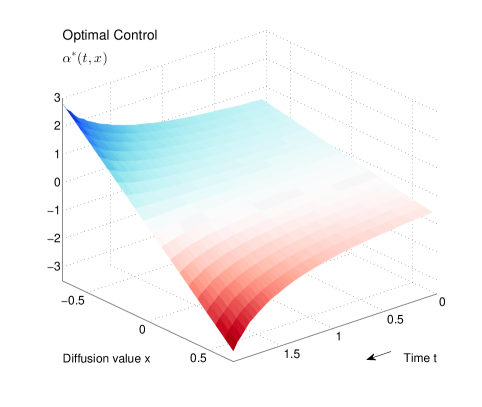
(a) Shape

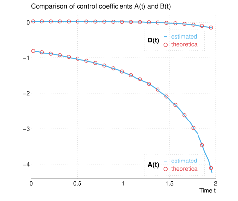
(b) Optimal coefficients vs. theoretical values

Figure 3.1: Optimal control

Figure 3.1a displays the shape of the optimal control $\alpha^{*}\left(t,x\right)$.

First, as expected from the drift term in the dynamics of $X^{\alpha}$ (equation (3.2)), $\alpha^{*}$ is a decreasing function of $x$ ($A\left(t\right)\leq 0$):

- If $X_{t}^{\alpha}$ takes a large positive value, then $\alpha^{*}\left(t,X_{t}\right)$ will take a large negative value so as to push it back more quickly to zero (recall the drift term $-\mu_{0}X_{s}^{\alpha}+\mu_{1}\alpha_{s}$).

- Conversely, if $X_{t}^{\alpha}$ takes a large negative value, then $\alpha^{*}\left(t,X_{t}\right)$ will take a large positive value for the same reason.

Second, the strength of the control increases as time reaches maturity (i.e. $A\left(t\right)$ decreases with $t$). Indeed, the penalization of the control becomes relatively cheaper compared with the penalization of the final value when time is close to maturity.

The strengthening of the control can also be assessed on Figure 3.1b, which displays the time evolution of the estimated coefficients $A$ and $B$ ($\alpha^{*}\left(t,x\right)=A\left(t\right)x+B\left(t\right)$). Moreover, one can see that the coefficient $B$ is slightly negative close to maturity. This creates an asymmetry in the control (as $\alpha^{*}\left(t,0\right)=B\left(t\right)\neq 0$), which comes from the asymmetric effect of the control on the volatility of $X^{\alpha}$.

The effect of the optimal control $\alpha^{*}$ is clearly visible on Figure 3.2 below, which compares the distribution of $X^{\alpha}$ without control (Figure 3.2a) and when the optimal control is used (Figure3.2b). The strengthening of the control at the end of the time period, as well as the slightly asymmetric shape of the distribution are prominent.

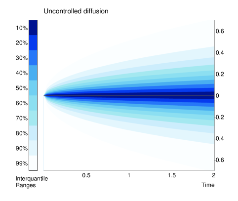
(a) Without control

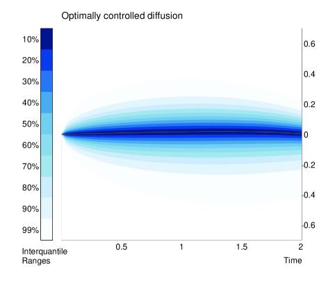
(b) With control

Figure 3.2: Time-evolution of the distribution of the diffusion

Finally, regarding the accuracy of the method, the comparison between the estimated coefficients and their theoretical values is reported on Figure 3.1b. Indeed an analytical characterization of the solution of linear quadratic stochastic control problems is available using ordinary differential equations (cf. [17]). On our one-dimensional example (3.1), it is given by:

$$\alpha^{*}\left(t,X_{t}\right) = A\left(t\right)X_{t}+B\left(t\right)$$

$$A\left(t\right) = -\frac{\mu_{1}P\left(t\right)}{2\lambda_{0}+\sigma_{1}^{2}P\left(t\right)}$$

$$B\left(t\right) = -\frac{\mu_{1}}{2\lambda_{0}}Q\left(t\right)+A\left(t\right)\left(\frac{\sigma_{0}\sigma_{1}}{\mu_{1}}-\frac{\sigma_{1}^{2}}{2\lambda_{0}}Q\left(t\right)\right)$$

where $P\left(t\right)$ and $Q\left(t\right)$ are the solutions of the following ordinary differential equations:

$$P^{\prime}\left(t\right) = 2\mu_{0}P\left(t\right)+\frac{\mu_{1}^{2}P^{2}\left(t\right)}{2\lambda_{0}+\sigma_{1}^{2}P\left(t\right)}$$

$$P\left(T\right) = 2\lambda_{1}$$

$$Q^{\prime}\left(t\right) = \left(\mu_{0}+\frac{\mu_{1}^{2}P\left(t\right)}{2\lambda_{0}+\sigma_{1}^{2}P\left(t\right)}\right)Q\left(t\right)+\frac{\sigma_{0}\sigma_{1}\mu_{1}P^{2}\left(t\right)}{2\lambda_{0}+\sigma_{1}^{2}P\left(t\right)}$$

$$Q\left(T\right) = 0$$

As can be seen from the comparison on Figure 3.1b, our estimates of the control coefficients are very accurate. Regarding the value function, our method provides the estimate $\hat{v}\left(0,0\right)=-5.761$. The theoretical value being equal to $-5.705$, this means a relative error of $1\%$.

3.2 Uncertain volatility/correlation model

The second application is the problem of pricing and hedging an option under uncertain volatility.

Instead of specifying the parameters of the dynamics of an underlying process, one can, for robustness, consider them uncertain. To some extent, this parameter uncertainty provides hedging strategies that are more robust to model risk (cf. [15]). To handle these uncertain parameters, the usual approach is to resort to superhedging strategies, that is, to find the smallest amount of money from which it is possible to superreplicate the option, i.e. to build a strategy that will almost surely provide an amount greater than (or equal to) the payoff at the maturity of the option.

To compute these prices in practice, the most common approach is to resort to numerical methods for partial differential equations. For instance, [12] computes the superhedging price under uncertain correlation of a digital outperformance option using a finite differences sheme. Unfortunately, these PDE methods suffer from the curse of dimensionality, which means that they cannot handle many state variables (no more than three in practice).

This is why a few authors tried recently to resort to Monte Carlo techniques to solve this problem of pricing and hedging options under uncertain volatility and/or correlation.

To our knowledge, the first attempt to do so was made in [13]. In this thesis, along the usual backward induction, the conditional expectation are computed using the Malliavin calculus approach. This approach uses the representation of conditional expectations in terms of a suitable ratio of unconditional expectations. Then, to find the optimal covariance matrix at each time step, an exhaustive comparison is performed. Of course, this methodology works only if the set of possible matrices is finite, which is the case when the optimal control is of bang-bang type. For instance, it includes the case of unknown correlations with known volatilies, but not the case when both volatilities and correlations are unknown, a shortcoming that is acknowledged in [13]. This means that this methodology can only deal with optimal switching problems, for which the control set is finite.

To overcome this limitation, [7] propose to restrict the maximization domain to a parameterized set of relevant functions, indexed by a low-dimensional parameter. They then perform this much simpler optimization inductively at each time step, by the downhill simplex method (when the optimum is not of bang-bang type). Once it is done, say, at time $t_{i}$, they immediately use these estimated volatilities and correlations (along with those from $t_{j}>t_{i}$) to resample the whole Monte Carlo set from $t_{i}$ to $T$ (and idea also used in the Multiple Step Forward scheme from [6]). Remark that this parameterization avoids the computation of conditional expectations for each point and time step.

In [7], a second Monte Carlo scheme is proposed. It is a Monte Carlo scheme for 2-BSDEs, very similar to the schemes [4] and [5], but fine-tuned for the uncertain volatility problem under log-normal processes. The conditional expectations are computed by parametric regression (non-parametric regression in dimension 1). Then for each point and each time step, a deterministic optimization procedure has to be performed to find the optimal covariance matrix. However, unlike in their previous algorithm, there is no resampling of the underlying diffusion using the newly computed covariances, which means that ensuring a proper simulation of the forward process becomes an issue.

Finally, we would like to draw attention to the work [14], which is not devoted to the uncertain volatility problem (it deals with the partial hedging of power futures with others futures with larger delivery period), but the numerical scheme they propose can deal with a control in the volatility. Their specific application allows to retrieve the optimal control by a fixed point argument, within a backward scheme. However, as in the previous algorithm, an a priori control has to be used to simulate the forward process.

In the present paper, our numerical scheme provides an alternative numerical sheme for dealing with the problem of pricing and hedging an option under uncertain volatility. To illustrate this, we implement it below on a simple example.

Consider two underlyings driven by the following dynamics:

$$dS_{i}\left(t\right) = \sigma_{i}S_{i}\left(t\right)dW_{i}\left(t\right)\,\,,\,\,i=1,2$$ (3.3)

$$\left\langle dW_{1}\left(t\right),dW_{2}\left(t\right)\right\rangle = \rho\left(t,S_{1}\left(t\right),S_{2}\left(t\right)\right)dt$$ (3.4)

where $\sigma_{1},\sigma_{2}>0$, $W_{1}$ and $W_{2}$ are two correlated brownian motions. We consider no drift and no interest rate for simplicity. We instead focus our attention on the following crucial feature: we consider the correlation $\rho$ to be uncertain. We only assume that $\rho$ always lies between two known bounds $-1\leq\rho_{\min}\leq\rho_{\max}\leq 1$:

$$\rho_{\min}\leq\rho\leq\rho_{\max}$$ (3.5)

Notice that when $\rho_{\min}$ $=$ $-1$ or $\rho_{\max}$ $=$ $1$, the diffusion matrix of $(S_{1},S_{2})$ can be degenerate.

We could also consider the two volatilities to be uncertain as well, but for illustration purposes, we focus on the uncertainty of the correlation parameter.

Finally, consider a payoff function $\Phi=\Phi\left(T,S_{1}\left(T\right),S_{2}\left(T\right)\right)$ at a time horizon $T>0$.

Now, the problem is to estimate the price of an option that delivers the payoff $\Phi$ at time $T$, and, if possible, to build a hedging strategy for this option.

Given that $\rho$ is uncertain, the model is incomplete, i.e. it is not possible to construct a hedging strategy that replicates perfectly the payoff $\Phi$ from any given amount of money. We thus look for superhedging strategies instead.

Hence, consider the class $\mathbf{Q}$ of all probability measures $\mathbb{Q}$ on the sets of paths $\left\{S_{i}\left(t\right)\right\}_{0\leq t\leq T}^{i=1,2}$ such that equations (3.4) and (3.5) hold for a particular $\rho^{\mathbb{Q}}$. The superhedging price is thus given by:

$$P_{0}^{+}:=\sup_{\mathbb{Q}\in\mathbf{Q}}\mathbb{E}^{\mathbb{Q}}\left[\Phi\left(T,S_{1}\left(T\right),S_{2}\left(T\right)\right)\right]$$ (3.6)

and the superhedging strategy is simply given by the usual delta-hedging strategy with $\rho$ equal to the correlation that attains the supremum in equation (3.6). In particular it provides an upper arbitrage bound to the price of the option. Symmetrically, a lower bound is provided by the subreplication price:

$$P_{0}^{-}:=\inf_{\mathbb{Q}\in\mathbf{Q}}\mathbb{E}^{\mathbb{Q}}\left[\Phi\left(T,S_{1}\left(T\right),S_{2}\left(T\right)\right)\right]$$ (3.7)

The practical computation of $P_{0}^{+}$ and $P_{0}^{-}$ falls within the scope of our numerical scheme.

We thus test our numerical scheme on this specific problem. We consider the example of a call spread on the spread $S_{1}\left(T\right)-S_{2}\left(T\right)$, i.e.:

$$\Phi=\left(S_{1}\left(T\right)-S_{2}\left(T\right)-K_{1}\right)^{+}-\left(S_{1}\left(T\right)-S_{2}\left(T\right)-K_{2}\right)^{+}$$

where $K_{1}<K_{2}$. Unless stated otherwise, the parameters of the model are fixed to the following values:

$S_{1}\left(0\right)$	$S_{2}\left(0\right)$	$\sigma_{1}$	$\sigma_{2}$	$\rho_{\min}$	$\rho_{\max}$	$K_{1}$	$K_{2}$	$T$
$50$	$50$	$0.4$	$0.3$	$-0.8$	$0.8$	$-5$	$5$	$0.25$

For the numerical parameters, we use $n=26$ time-discretization steps, and a sample of $M=10^{6}$ Monte Carlo simulations. For the regressions, we use a basis function of sigmoid transforms of polynomial of degree two:

$$\phi\left(t,s_{1},s_{2},\rho\right) := \left(K_{2}-K_{1}\right)\times\mathcal{S}\left(\beta_{0}+\beta_{1}s_{1}+\beta_{2}s_{2}+\beta_{3}\rho+\beta_{4}\rho s_{1}+\beta_{5}\rho s_{2}\right)$$

$$\mathcal{S}\left(u\right) := \frac{1}{1+e^{-u}}$$

We chose the sigmoid function for its resemblance to the call spread payoff, and the terms inside the sigmoid according to their statistical significance. With this choice of basis, the optimal control will be bang-bang:

$$\rho^{*} =\rho^{*}\left(t,s_{1},s_{2}\right):=\arg\max_{\rho}\phi\left(t,s_{1},s_{2},\rho\right)=\rho_{\max}\mathbf{1}\left\{\beta_{3}+\beta_{4}s_{1}+\beta_{5}s_{2}\geq 0\right\}+\rho_{\min}\mathbf{1}\left\{\beta_{3}+\beta_{4}s_{1}+\beta_{5}s_{2}<0\right\}$$

Figure 3.3 below reports our results.

Figure 3.3a reports the superhedging and subhedging prices of the option, for different values of the moneyness ($S_{2}\left(0\right)=50$ is kept fixed and different values of $S_{1}\left(0\right)=50+{\rm Moneyness}$ are tested). One can clearly see the range of non-arbitrage prices that they define. For comparison, the prices obtained when $\rho$ is constant are reported on the same graph for different values ($\rho_{\min}$, $0$ and $\rho_{\max}$). One can see that, even though these prices belong to the non-arbitrage range, they do not cover the whole range, especially close to the money. This clearly indicates that, as already observed in [12] for instance, the practice of pricing under the hypothesis of constant parameters, and then testing different values for the parameters can be a very deceptive assessment of risk (as “uncertain” is not the same as “uncertain but constant”).

Figure 3.3b illustrates the impact of the size of the correlation range $\left[\rho_{\min},\rho_{\max}\right]$. Naturally, the wider the correlation range, the wider the price range. On average, an increase of 0.1 of the correlation range increases the price range by $0.135$.

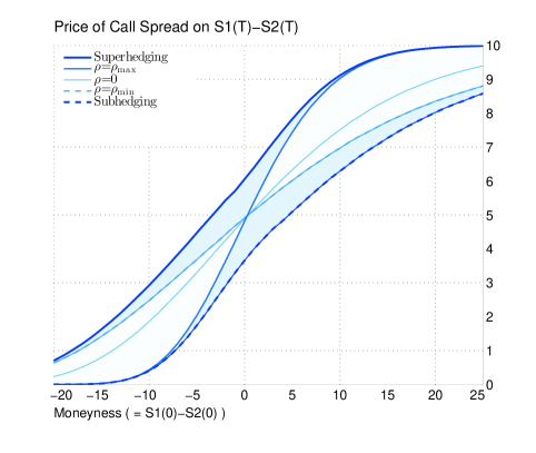
(a) Price of Call Spread

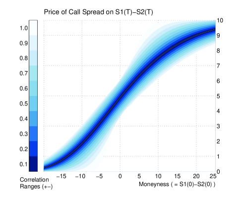
(b) Influence of the correlation range

Figure 3.3: Prices under uncertain correlation

3.3 Comparisons with [7]

Finally, we test our algorithm on several payoffs proposed in [7], and compare the behaviour of our method to their results. To be more specific, we will not focus our comparison of algorithms to their parametric approach, but to their second-order BSDE approach, as both algorithms are similar in nature (forward-backward schemes involving simulations and regressions).

Actually, we are going to implement and compare two different versions of our scheme. The first one correspond to the empirical version of the scheme studied in Section 2:

$$\hat{Y}_{N} =g\left(X_{N}\right)$$

$$\hat{\mathcal{Y}}_{i} =\hat{\mathbb{E}}_{i}\left[\hat{Y}_{i+1}+f\left({\color[rgb]{0,0,0}X_{i}},I_{i}\right)\Delta_{i}\right]$$

$$\hat{Y}_{i} =\underset{a\in A}{\mathrm{ess\,sup\,}}\mathbb{E}_{i,a}\left[\hat{\mathcal{Y}}_{i}\right]$$ (3.8)

where $\hat{\mathbb{E}}_{i}$ corresponds to an empirical least-squares regression which approximates the true conditional expectation $\mathbb{E}_{i}$. In the simpler context of American option pricing, this scheme would correspond to the Tsitsiklis-van Roy algorithm ([16]).

The second one makes use of the estimated optimal policies computed by the first algorithm, which are then directly plugged into the stochastic control problem under consideration:

$$\hat{\alpha}_{i} =\arg\underset{a\in A}{\mathrm{ess\,sup\,}}\mathbb{E}_{i,a}\left[\hat{\mathcal{Y}}_{i}\right]$$

$$\hat{X}_{i+1} =b(\hat{X}_{i},\hat{\alpha}_{i})\Delta_{i}+\sigma(\hat{X}_{i},\hat{\alpha}_{i})\Delta W_{i}$$

$$\hat{v}\left(t_{0},x_{0}\right) =\frac{1}{M}\sum_{m=1}^{M}\left[\sum_{i=1}^{N}f(\hat{X}_{i+1},\hat{\alpha}_{i})\Delta_{i}+g(\hat{X}_{N})\right]$$ (3.9)

In the context of American option pricing, this scheme would correspond to the Longstaff-Schwarz algorithm ([11]).

We compute both prices as they are somehow complementary. Indeed, as noticed in [3] and detailed in [1], the first algorithm tend to be upward biased (up to the Monte Carlo error and the regression bias) compared with the discretized price, while the second one tend to be downward biased (up to the Monte Carlo error). Therefore, computing both prices provides a kind of empirical confidence interval, with the length of the interval being due to the choice of regression basis, thus providing an empirical assessment of the quality of the chosen regression basis.

Call Spread

Let $S$ be a geometric brownian motion with $S\left(0\right)=100$ and with uncertain volatility $\sigma$ taking values in $\left[0.1,0.2\right]$.

Consider a call spread option, with payoff $\left(S\left(T\right)-K_{1}\right)^{+}-\left(S\left(T\right)-K_{2}\right)^{+}$ and time horizon $T=1$, with $K1=90$ and $K2=110$. The true price of the option (as estimated by PDE methods in [7]) is $\mathcal{C}_{PDE}=11.20$, and the Black-Scholes price with constant volatility $\sigma_{\mathrm{mid}}=0.15$ is $\mathcal{C}_{BS}=9.52$. We implement our scheme using the following set of basis functions:

$$\phi\left(t,s,\sigma\right)=\left(K_{2}-K_{1}\right)\times\mathcal{S}\left(\beta_{0}+\beta_{1}s+\beta_{2}s^{2}+\beta_{3}\sigma+\beta_{4}\sigma s+\beta_{5}\sigma s^{2}\right)$$

where, as in Subsection 3.2, $\mathcal{S}$ denotes the sigmoid function.

Figure 3.4 describes the estimates obtained with both algorithms (3.8) and (3.9), for various values of the number $M$ of Monte Carlo simulations, and of the length of the constant discretization time step. For comparison, the red line corresponds to the price $\mathcal{C}_{PDE}$ of the option.

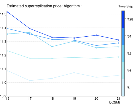
(a) First Algorithm

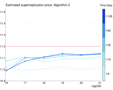
(b) Second Algorithm

Figure 3.4: Price of Call Spread

The following general observations can be made.

First, for a small enough time step, the prices computed using the first algorithm (3.8) (Figure 3.4a) tend as expected to be above the true price, while the second algorithm (3.9) (Figure 3.4b) tend to be below it.

Our best estimate here ($M=2^{21}$ , $\Delta_{t}=1/128$) is $11.31$ with the first algorithm ($+1\%$ compared with the true price) and $11.14$ with the second one ($-0.6\%$). The true price lies indeed between those two bounds, and their average ($11.22$) is even closer to the true price than any of the two estimates ($+0.2\%$).

The prices computed with the first algorithm always lie above the prices computed with the second algorithm. As these prices are expected to surround the true discretized price (as would be computed by the scheme (3.8) with $\mathbb{E}_{i}$ instead of $\hat{\mathbb{E}}_{i}$), the fact that for large discretization steps ($\Delta_{t}=1/8$ or $1/16$) the prices computed using the first algorithm are below the true price $11.20$ simply means that, for such discretization steps, the true discretized price lies below the true price (in other words the time discretization generates here a negative bias).

Finally, increasing the number of Monte Carlo simulations tends as expected to improve the price estimates. However, the Monte Carlo error can be negligible compared with the discretization error for small time steps, which is why both a large number of Monte Carlo simulations and a small discretization time step are required to obtain accurate estimates.

In [7], the algorithm based on second-order BSDEs produces the estimates $11.04$ for $\left(1/\Delta_{t},\log_{2}\left(M\right)\right)=\left(8,16\right)$ and $11.11$ for $\left(1/\Delta_{t},\log_{2}\left(M\right)\right)=\left(8,17\right)$. This is close to our estimates for similar parameters. However, a more accurate comparison would require to test their algorithm with smaller time steps and more Monte Carlo simulations (they only consider parameters $\left(1/\Delta_{t},\log_{2}\left(M\right)\right)$ within $\left[2,8\right]\times\left[12,17\right]$, whereas we consider here the range $\left[8,128\right]\times\left[16,21\right]$, as it provides much greater accuracy of the estimates, providing a sound basis for the analysis of the results).

Digital option:

Consider a digital option, with payoff $100\times\mathbf{1}\left\{S\left(T\right)\geq K\right\}$ and $T=1$ on the samee asset, with $K=100$. The true (PDE) price is $\mathcal{C}_{PDE}=63.33$, and the Black-Scholes price with mid-volatility is $\mathcal{C}_{BS}=46.54$. We use the following set of basis functions:

$$\phi\left(t,s,\sigma\right)=100\times\mathcal{S}\left(\beta_{0}+\beta_{1}s+\beta_{2}s^{2}+\beta_{3}\sigma+\beta_{4}\sigma s+\beta_{5}\sigma s^{2}\right)$$

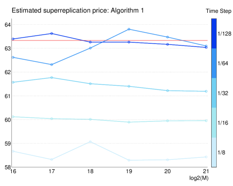
(a) First Algorithm

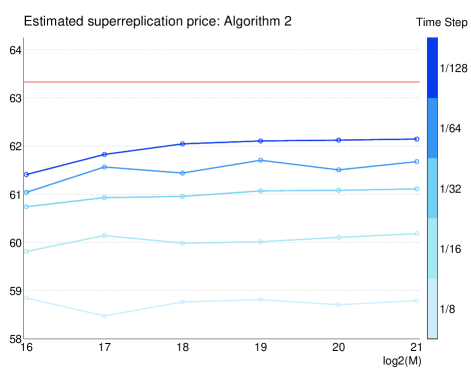
(b) Second Algorithm

Figure 3.5: Price of Digital Option

As can be seen on Figure 3.5, the time discretization error is much more pronounced with this discontinuous payoff, compared with the previous call spread example. We manage to reach estimates of $63.04$ ($-0.5\%$) and $62.15$ ($-1.9\%$), even though smaller time steps would be required for better accuracy.

For small parameters ($\left(1/\Delta_{t},\log_{2}\left(M\right)\right)=\left(8,16\right)$), the accuracy is better in [7] ($60.53$), even though shortening the time step tends to degrade the results in their case.

Outperformer Option:

Consider now two geometric Brownian motions $S_{1}$ and $S_{2}$, starting from $100$ at time $0$, with uncertain volatilities $\sigma_{1}$ and $\sigma_{2}$ taking values in $\left[0.1,0.2\right]$. For the moment, suppose that the correlation $\rho$ between the two underlying Brownian motions is zero.

Consider an outperformer option, with payoff $\left(S_{1}\left(T\right)-S_{2}\left(T\right)\right)^{+}$ and time horizon $T=1$. The true price is $\mathcal{C}=11.25$. We use the following set of basis functions:

$$\phi\left(t,s_{1},s_{2},\sigma_{1},\sigma_{2}\right)= 100\times\left(\beta_{0}+\beta_{1}s_{1}+\beta_{2}s_{1}^{2}+\beta_{3}s_{2}+\beta_{4}s_{2}^{2}+\beta_{5}s_{1}s_{2}+\beta_{6}\sigma_{1}+\beta_{7}\sigma_{1}s_{1}+\beta_{8}\sigma_{1}s_{1}^{2}\right.$$

$$\left.+\beta_{9}\sigma_{1}s_{2}+\beta_{10}\sigma_{1}s_{2}^{2}+\beta_{11}\sigma_{2}+\beta_{12}\sigma_{2}s_{1}+\beta_{13}\sigma_{2}s_{1}^{2}++\beta_{14}\sigma_{2}s_{2}+\beta_{15}\sigma_{2}s_{2}^{2}\right)$$

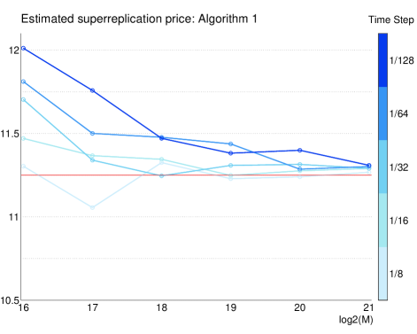
(a) First Algorithm

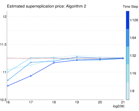
(b) Second Algorithm

Figure 3.6: Price of Outperformer Option ($\rho=0$)

Here, in contrast with the previous examples, the bulk of the error comes from the Monte Carlo simulations, and not from the time discretization. Moreover, both algorithms provide very accurate estimates. Indeed, this convex option is easy to price under the uncertain volatility model, as it is given by the price obtained with the maximum volatilities. With our choice of regression basis, the algorithm correctly detects that the maximum volatilities are to be used, leading to these very accurate estimates $11.31$ ($+0.5\%$) and $11.25$ ($-0\%$). For the same reason, the estimates from [7] are accurate too.

Figure 3.7 below depicts the estimated price of the same option but now with a negative constant correlation $\rho=-0.5$. Its true price is $\mathcal{C}=13.75$.

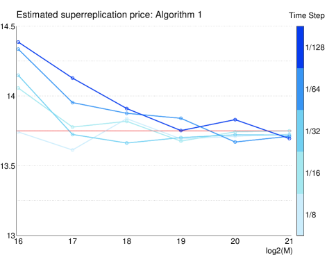
(a) First Algorithm

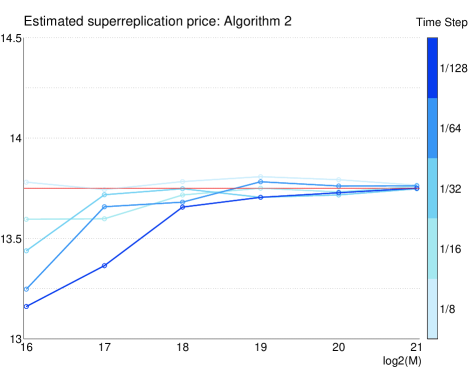
(b) Second Algorithm

Figure 3.7: Price of Outperformer Option ($\rho=-0.5$)

The same behaviour can be observed. Both algorithms are accurate here ($13.69$ ($-0.4\%$) and $13.75$ ($-0\%$)).

As the estimate from the first algorithm happens to lie below the true price, we take advantage of this result to recall from the introduction of this subsection that the bias of the first algorithm bears one more source of error (the regression bias) than the bias of the second algorithm. This means that in general the sign of the bias wrt. the true discretized price is more reliable with the second algorithm. With this observation in mind, we propose, from the two estimates $P_{1}$ and $P_{2}$ computed by the two algorithms, to consider the following general estimate $P$:

$$P:=\max\left(P_{2},\frac{P_{1}+P_{2}}{2}\right)$$

Indeed, if $P_{1}\geq P_{2}$ (which is the expected behaviour), then $P:=\frac{P_{1}+P_{2}}{2}$ may provide a better estimate than both $P_{1}$ and $P_{2}$ separately (as is the case for the call spread example from Figure 3.4). However, when $P_{1}<P_{2}$ (which is not expected), then, recalling that $P_{2}$ may be more accurate than $P_{1}$, it is better to consider $P:=P_{2}$ (as is the case here of this outperformer option with $\rho=-0.5$). In the following, we will call $P$ the mid-estimate (with a slight abuse of terminology, as $P$ is usually but not always the average between $P_{1}$ and $P_{2}$).

Outperformer spread option:

We now analyze a more complex payoff. Consider an outperformer spread option, with payoff $\left(S_{2}\left(T\right)-K_{1}S_{1}\left(T\right)\right)^{+}-\left(S_{2}\left(T\right)-K_{2}S_{1}\left(T\right)\right)^{+}$, time horizon $T=1$ and constant correlation $\rho=-0.5$. The true (PDE) price is $\mathcal{C}_{PDE}=11.41$, and the Black-Scholes price with mid-volatility is $\mathcal{C}_{BS}=9.04$. We use the following set of basis functions:

$$\phi\left(t,s_{1},s_{2},\sigma_{1},\sigma_{2}\right)=s_{1}\times\left(K_{2}-K_{1}\right)\times \mathcal{S}\left(\beta_{0}+\beta_{1}\frac{s_{2}}{s_{1}}+\beta_{2}\left(\frac{s_{2}}{s_{1}}\right)^{2}+\beta_{3}\sigma_{1}+\beta_{4}\sigma_{1}\frac{s_{2}}{s_{1}}+\beta_{5}\sigma_{1}\left(\frac{s_{2}}{s_{1}}\right)^{2}\right.$$

$$\left.+\beta_{6}\sigma_{2}+\beta_{7}\sigma_{2}\frac{s_{2}}{s_{1}}+\beta_{8}\sigma_{2}\left(\frac{s_{2}}{s_{1}}\right)^{2}\right)$$

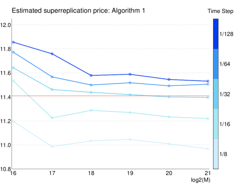
(a) First Algorithm

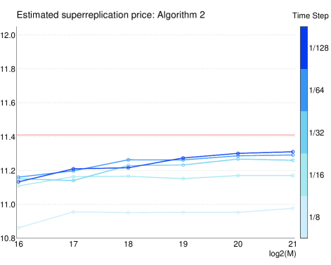
(b) Second Algorithm

Figure 3.8: Price of Outperformer Spread Option ($\rho=-0.5$)

In this example, one can see that the time discretization produces a large downward bias (as in the call spread and digital option examples), but both algorithms behave as expected (the first algorithm produces high estimates, the second produces low estimates, and both are close to the true price ($11.53$ ($+1\%$) and $11.31$ ($-0.9\%$))). Moreover, the mid-estimate $11.42$ is very accurate.

In [7] is reported the estimate $10.83$ for $\left(1/\Delta_{t},\log_{2}\left(M\right)\right)=\left(8,20\right)$, which is slightly worse than our estimates for the same choice of $M$ and $\Delta_{t}$ ($11.01$ and $10.95$), but the difference can be due to the different choice of basis. However, the three estimates are well below the true price, and our numerical results indicate that the reason is that $\Delta_{t}=1/8$ is too large a time step.

This suggests that the estimates from [7] could be improved by considering smaller time steps. However, as acknowledged in their paper, the second-order BSDE method does not work properly when $\Delta_{t}$ is too small. Indeed, their BSDE scheme makes use of the first order component $Z$ and the second order component $\Gamma$. The problem here is that, for fixed $M$, the variance of the estimators of $Z$ and $\Gamma$ tends to infinity when $\Delta_{t}$ tends to zero. However, as detailed in [2], this problem can be completely solved by amending the estimators using appropriate variance reduction terms. Therefore, in our opinion, a fair comparison of the jump-constrained BSDE approach and the second-order BSDE approach would require the use of the variance reduction method from [2] to allow for smaller time steps for the second-order BSDE approach.

As a final numerical example, we consider again the same outperformer spread option, with the exception that the correlation $\rho$ is now considered uncertain, within $\left[-0.5,0.5\right]$. The true (PDE) price is $\mathcal{C}_{\mathrm{PDE}}=12.83$, and the Black-Scholes price with mid-volatility is $\mathcal{C}_{BS}=9.24$. We use the following basis functions:

$$\phi\left(t,s_{1},s_{2},\sigma_{1},\sigma_{2},\rho\right)=s_{1}\times\left(K_{2}-K_{1}\right)\times \mathcal{S}\left(\beta_{0}+\beta_{1}\frac{s_{2}}{s_{1}}+\beta_{2}\left(\frac{s_{2}}{s_{1}}\right)^{2}+\beta_{3}\sigma_{1}+\beta_{4}\sigma_{1}\frac{s_{2}}{s_{1}}+\beta_{5}\sigma_{1}\left(\frac{s_{2}}{s_{1}}\right)^{2}\right.$$

$$\left.+\beta_{6}\sigma_{2}+\beta_{7}\sigma_{2}\frac{s_{2}}{s_{1}}+\beta_{8}\sigma_{2}\left(\frac{s_{2}}{s_{1}}\right)^{2}+\beta_{6}\rho+\beta_{7}\rho\frac{s_{2}}{s_{1}}+\beta_{8}\rho\left(\frac{s_{2}}{s_{1}}\right)^{2}\right)$$

Remark that at each time step we perform here a five-dimensional regression.

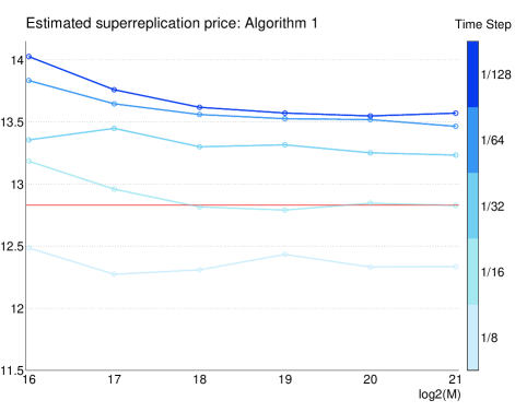
(a) First Algorithm

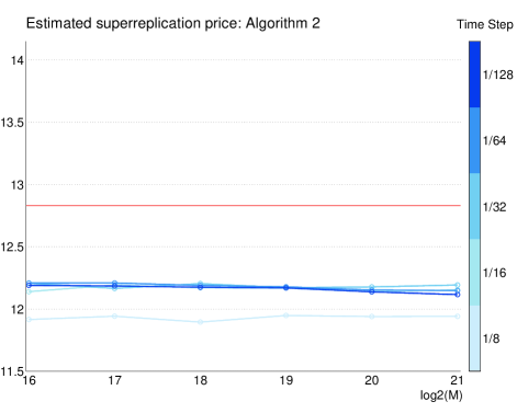
(b) Second Algorithm

Figure 3.9: Price of Outperformer Spread Option ($\rho$ uncertain $\in\left[-0.5,0.5\right]$)

On this example, we observe a wide gap between the two estimates $13.57$ ($+5.8\%$) and $12.12$ ($-5.6\%$) ($\left(1/\Delta_{t},\log_{2}\left(M\right)\right)=\left(128,21\right)$). As neither the number of Monte Carlo simulation nor the discretization time step seem able to narrow the gap, it means that it is due to the chosen regression basis. Indeed, our basis is such that the optimal volatilities and correlation are of bang-bang type, as in the previous examples. However, unlike the previous examples, here both the volatilities and the correlation are uncertain, and in this case it is known (cf. [13] for instance) that the optimum is not of a bang-bang type. Therefore, one should look for a richer regression basis in order to narrow the estimation gap on this specific example. Remark however that the mid-estimated $12.84$ remains very accurate. On the same example and with another regression basis, [7] manage to reach a price of $12.54$ for $\left(1/\Delta_{t},\log_{2}\left(M\right)\right)=\left(8,20\right)$.

To conclude these subsection, here are the differences we could notice between the jump-constrained BSDE approach and the second-order BSDE approach applied to the problem of pricing by simulation under uncertain volatility model:

• Both are forward-backward schemes. Thus, the first step is to simulate the forward process. At this stage the jump-constrained BSDE approach is advantaged, because its forward process is a simple Markov process, therefore easy to simulate. Its randomization of the control is fully justified mathematically. On the contrary, the second-order BSDE requires to resort to heuristics in order to simulate the forward process despite the fact that the control is involved in its dynamics. [7] propose to use an arbitrary constant volatility (the mid-volatility) to simulate the forward process, and they notice that the specific choice of prior-volatility does impact substantially the resulting estimates.

• Then comes the estimation of the backward process. If both schemes require to perform regressions, this step is more difficult in the jump-constrained BSDE approach, because the dimensionality of the regressions is higher as the state process contains the randomized controls. In particular the choice of regression basis is more difficult.

• On the set of options considered here and within the same range of numerical parameters $M$ and $\Delta_{t}$ we could not detect any significant and systematic difference between the two algorithms. Nevertheless, we strongly suggest the following two points:

• First, the second-order BSDE approach would strongly benefit from the use of the variance reduction method from [2]. It would allow for smaller time steps to be considered, and therefore allow for a sounder and more precise numerical comparison between the two approaches. Indeed, the accurate estimates recorded in [7] for very large time steps may be, as in Figure 3.9a for $\Delta_{t}=1/16$, an incidental cancellation of biases of opposite signs. The significant quantity is the level where the estimates converge for small $\Delta_{t}$.

• Second, to complement the downward biased, “Longstaff-Schwartz like” estimator considered in [7], we suggest the computation of the upward biased, “Tsitsiklis-van Roy like” estimator, as we did in this paper, as both estimators appear to be informative in a complementary fashion, and the mid-estimator proposed here (which requires both estimators) seems to perform staggeringly well.

4 Conclusion

We proposed in this paper a general probabilistic numerical algorithm, combining Monte Carlo simulations and empirical regressions, which is able to solve numerically very general HJB equations in high dimension. That includes general stochastic control problems with controlled volatility, possibly degenerate, but more generally, it can solve any jump-constrained BSDE ([9]).

We initiated a partial analysis of the theoretical error of the scheme, and we provided several numerical application of the scheme on the problem of pricing under uncertain volatility, the results of which are very promising.

In the future, we would like to extend this work in the following direction:

• First, we would like to manage to obtain a comprehensive analysis of the error of the scheme, including the empirical regression step.

• Then, we would like to perform a more systematic numerical comparison with the alternative scheme described in [7], taking into account our empirical findings.

• Finally, we would like to extend the general methodology of control randomization and subsequent constraint on resulting jumps to more general problems, like HJB-Isaacs equations or even mean-fields games, with possible advances on the numerical solution of such problems.

References

- [1] R. Aïd, L. Campi, N. Langrené, and H. Pham. A probabilistic numerical method for optimal multiple switching problem in high dimension. Preprint, 2012.
- [2] S. Alanko and M. Avellaneda. Reducing variance in the numerical solution of BSDEs. Comptes Rendus Mathematique, 351(3-4):135–138, 2013.
- [3] B. Bouchard and X. Warin. Monte-Carlo valorisation of American options: facts and new algorithms to improve existing methods. In R. Carmona, P. Del Moral, P. Hu, and N. Oudjane, editors, Numerical Methods in Finance, volume 12 of Springer Proceedings in Mathematics, 2012.
- [4] P. Cheridito, M. Soner, N. Touzi, and N. Victoir. Second order backward stochastic differential equations and fully non-linear parabolic PDEs. Communications on Pure and Applied Mathematics, 60(7):1081–1110, 2007.
- [5] A. Fahim, N. Touzi, and X. Warin. A probabilistic numerical method for fully nonlinear parabolic PDEs. The Annals of Applied Probability, 21(4):1322–1364, 2011.
- [6] E. Gobet and P. Turkedjiev. Approximation of discrete BSDE using least-squares regression. Preprint, 2011.
- [7] J. Guyon and P. Henry-Labordère. Uncertain volatility model: a Monte Carlo approach. The Journal of Computational Finance, 14(3):37–71, 2011.
- [8] I. Kharroubi, N. Langrené, and H. Pham. A numerical algorithm for fully nonlinear HJB equations: an approach by control randomization. Preprint, 2013.
- [9] I. Kharroubi and H. Pham. Feynman-Kac representation for Hamilton-Jacobi-Bellman IPDE. Preprint, 2012.
- [10] J.-P. Lemor, E. Gobet, and X. Warin. Rate of convergence of an empirical regression method for solving generalized backward stochastic differential equations. Bernoulli, 12(5):889–916, 2006.
- [11] F. Longstaff and E. Schwartz. Valuing American options by simulation: a simple least-squares approach. Review of Financial Studies, 14(1):113–147, 2001.
- [12] J. Marabel. Pricing digital outperformance options with uncertain correlation. International Journal of Theoretical and Applied Finance, 14(5):709–722, 2011.
- [13] M. Mrad. Méthodes numériques d’évaluation et de couverture des options exotiques multi-sous-jacents : modèles de marché et modèles à volatilité incertaine. PhD thesis, University of Paris 1 Pantheon-Sorbonne, 2008.
- [14] A. Nguyen Huu and N. Oudjane. Hedging expected losses on derivatives in electricity Futures markets. Preprint, 2013.
- [15] D. Talay. Model risk in finance: some modelling and numerical analysis issues. In A. Bensoussan and Q. Zhang, editors, Mathematical Modeling and Numerical Methods in Finance, volume 15 of Handbook of Numerical Analysis, pages 3–28, 2008.
- [16] J. Tsitsiklis and B. Van Roy. Regression methods for pricing complex American-style options. IEEE Transactions on Neural Networks, 12(4):694–703, 2001.
- [17] J. Yong and X. Zhou. Stochastic Controls: Hamiltonian Systems and HJB Equations. Springer, 1999.
- [18] D. Zanger. Quantitative error estimates for a least-squares Monte Carlo algorithm for American option pricing. Preprint, 2012.