Probability distribution for the relative velocity of colliding particles in a relativistic classical gas

Abstract

We find the probability density function $\mathcal{P}(V_{\texttt{r}})$ of the relativistic relative velocity for two colliding particles in a non-degenerate relativistic gas. The distribution reduces to Maxwell distribution for the relative velocity in the non-relativistic limit. We find an exact formula for the mean value $\langle V_{\texttt{r}}\rangle$. The mean velocity tends to the Maxwell’s value in the non-relativistic limit and to the velocity of light in the ultra-relativistic limit. At a given temperature $T$, when at least for one of the two particles the ratio of the rest energy over the thermal energy $mc^{2}/k_{B}T$ is smaller than 40 the Maxwell distribution is inadequate.

I Introduction

In many fields of physics and astrophysics one has to study reaction rates in a system that can be considered, to a good approximation, a classical non-relativistic gas in equilibrium. In the gas can be present different species of particles. We consider two species with masses $m_{1}$ and $m_{2}$ and number densities $n_{1,2}$, the number of particles per unit volume. For a given process with total cross section $\sigma$, the number of reactions per unit time per unit volume, the reaction rate, is given by $R=n_{1}n_{2}\sigma v_{{r}}$, where

$$v_{{r}}=\rvert\boldsymbol{v}_{1}-\boldsymbol{v}_{2}\rvert$$ (1)

is the relative velocity between two particles with velocities $\boldsymbol{v}_{1}$ and $\boldsymbol{v}_{2}$. The cross section is in general function of the relative velocity but we will not write explicitly the dependence. As it is well known, at a given temperature $T$ units , the absolute velocity of the particles follows the Maxwell distribution $f_{M}(v)=(2/\pi)^{1/2}(m/T)^{3/2}v^{2}\exp(-mv^{2}/(2T))$. The thermally averaged reaction rate then is

$$\langle R\rangle=n_{1}n_{2}\int d\boldsymbol{v}_{1}d\boldsymbol{v}_{2}f_{M}({v}_{1})f_{M}({v}_{2})\sigma{v}_{{r}}.$$ (2)

By changing variables from the velocities $\boldsymbol{v}_{1}$, $\boldsymbol{v}_{2}$ to the velocity of the center of mass $\boldsymbol{v}_{c}$ and the relative velocity $\boldsymbol{v}_{r}$, one finds the standard expression for the thermal averaged rate,

$$\langle R\rangle=n_{1}n_{2}\int_{0}^{\infty}dv_{{r}}F_{\text{M}}(v_{{r}})\sigma v_{{r}},$$ (3)

where

$$F_{{M}}(v_{{r}})=\sqrt{\frac{2}{\pi}}\left(\frac{\mu}{T}\right)^{3/2}{v}^{2}_{{r}}\,e^{-\mu\frac{v_{{r}}^{2}}{2T}}$$ (4)

is the distribution of the relative velocity. Equation (4) has the same form of the Maxwell distribution for the absolute velocity but with the reduced mass $\mu=m_{1}m_{2}/(m_{1}+m_{2})$ in place of $m$ and $v_{{r}}$ in place of $v$.

If the colliding particles are relativistic corrections to Eq. (2) can be important. On the other hand, conceptually, both the relative velocity (1) and the Maxwell distribution (4) are not compatible with the fact that $v_{r}$ for two massive particles must be smaller than velocity of light $c$ in every inertial frame, while the relative velocity between two massless particles and between a massless and a massive particle is always equal to the velocity of light.

It is thus interesting to ask if a probability distribution for the relative velocity compatible with the principles of special relativity exists. In this paper we show that such a distribution exists and that $F_{{M}}(v_{{r}})$ is just its non-relativistic limit.

Let us remind first how the previous discussion of the non-relativistic reaction rate is reformulated in a Lorentz invariant way. The relativistic relative velocity is Landau2 ; Cercignani

$$V_{\texttt{r}}=\frac{\sqrt{(\boldsymbol{v}_{1}-\boldsymbol{v}_{2})^{2}-(\boldsymbol{v}_{1}\times\boldsymbol{v}_{2})^{2}}}{1-\boldsymbol{v}_{1}\cdot\boldsymbol{v}_{2}}.$$ (5)

This expression is symmetric in the two velocities in any frame and have all the required properties. In the non-relativistic limit $V_{\texttt{r}}$ reduces to (1). The Lorentz invariant rate is Landau2 ; Cercignani

$$\mathcal{R}=n_{1}n_{2}\frac{p_{1}\cdot p_{2}}{E_{1}E_{2}}\sigma V_{\texttt{r}},$$ (6)

where $p_{i}=(E_{i},\boldsymbol{p}_{i})$, $E_{i}=\sqrt{\boldsymbol{p}^{2}_{i}+m^{2}_{i}}$, $i=1,2$, are the four-momentum of the colliding particles.

A relativistic non-degenerate gas in equilibrium is described by the relativistic generalization of the Maxwell distribution, the Jüttner distribution juttner ; DeGroot ; csernai ; Cercignani . The normalized momentum distribution is given by

$$f_{J}(\boldsymbol{p})=\frac{1}{4\pi m^{2}TK_{2}(x)}e^{-\frac{u\cdot p}{T}}.$$ (7)

Here and in what follows, $K_{n}(x)$ are modified Bessel functions of the second kind of order $n$, and $u$ a time-like four-velocity of the gas such that $u\cdot u=1$. Averaging the rate (6) with the Jüttner distribution (7), the relativistic analogous of Eq. (2) hence is

$$\langle\mathcal{R}\rangle=n_{1}n_{2}\int\frac{d^{3}\boldsymbol{p}_{1}}{E_{1}}\frac{d^{3}\boldsymbol{p}_{2}}{E_{2}}f_{J}(\boldsymbol{p}_{1})f_{J}(\boldsymbol{p}_{2})\,(p_{1}\cdot p_{2})\sigma V_{\texttt{r}}.$$ (8)

This is our starting point.

II Probability distribution for the relative velocity

In Eq. (8) the integrand is manifestly Lorentz invariant. In order to simplify the calculation, we can choose the so-called Lorentz local rest frame DeGroot ; Cercignani ; csernai where the four velocity of the gas is $u=(1,\boldsymbol{0})$. Hence, (1) we show that

$$\int\frac{d^{3}\boldsymbol{p}_{1}}{E_{1}}\frac{d^{3}\boldsymbol{p}_{2}}{E_{2}}{p_{1}\cdot p_{2}}f_{J}(\boldsymbol{p}_{1})f_{J}(\boldsymbol{p}_{2})\equiv\int^{1}_{0}dV_{\texttt{r}}\mathcal{P}_{\texttt{r}}(V_{\texttt{r}})=1;$$

(2) we give the explicit expression for $\mathcal{P}_{\texttt{r}}(V_{\texttt{r}})$; (3) we verify $\mathcal{P}_{\texttt{r}}(V_{\texttt{r}})$ in the non-relativistic limit reduces to Eq. (4).

(1) Introducing the ratios $x_{i}=m_{i}/T$ we have

$$\Phi=\frac{\int\frac{d^{3}\boldsymbol{p}_{1}}{E_{1}}\frac{d^{3}\boldsymbol{p}_{2}}{E_{2}}p_{1}\cdot p_{2}e^{-\frac{E_{1}+E_{2}}{T}}}{(4\pi T)^{2}\prod_{i}m^{2}_{i}K_{2}(x_{i})}=\frac{\mathcal{N}}{\mathcal{D}}.$$ (9)

The integrand in the numerator depends on $\theta$, the angle between $\boldsymbol{p}_{1}$ and $\boldsymbol{p}_{2}$, trough the scalar product $p_{1}\cdot p_{2}$. Passing in polar coordinates in momentum space, $d^{3}\boldsymbol{p}_{1}=4\pi|\boldsymbol{p}_{1}|^{2}d|\boldsymbol{p}_{1}|$, $d^{3}\boldsymbol{p}_{2}=2\pi|\boldsymbol{p}_{2}|^{2}d|\boldsymbol{p}_{1}|d\cos\theta$, the integration over the angle gives

$$\int^{1}_{-1}d\cos\theta(E_{1}E_{2}-|\boldsymbol{p}_{1}||\boldsymbol{p}_{2}|\cos\theta)=2E_{1}E_{2}.$$

The numerator is thus $\mathcal{N}=\prod_{i}\int d^{3}\boldsymbol{p}_{i}e^{-\frac{E_{i}}{T}}=\mathcal{D}$ because of the normalization of the Jüttner distribution (7). It follows that $\Phi=1$.

(2) To find the explicit expression for $\mathcal{P}_{\texttt{r}}(V_{\texttt{r}})$ it is convenient to follow Refs. GG and change variables from $E_{1}$, $E_{2}$, $\cos\theta$ to $Y=E_{1}+E_{2}$, $Z=E_{1}-E_{2}$ and the Mandelstam invariant $s=(p_{1}+p_{2})^{2}$. Defining

$$p^{\prime}=\frac{\sqrt{s-(m_{1}+m_{2})^{2}}\sqrt{s-(m_{1}-m_{2})^{2}}}{2\sqrt{s}}.$$ (10)

and $M=m_{1}+m_{2}$, with $p_{1}\cdot p_{2}=[s-(m^{2}_{1}+m^{2}_{2})]/2$, we obtain

$$\Phi=\frac{\int_{M^{2}}^{\infty}ds[s-(m^{2}_{1}+m^{2}_{2})]p^{\prime}K_{1}(\sqrt{s}/T)}{4T\prod_{i}m^{2}_{i}K_{2}(x_{i})}.$$ (11)

Introducing the Lorentz factor associated with $V_{\texttt{r}}$,

$$\gamma_{\texttt{r}}=\frac{1}{\sqrt{1-v^{2}_{\texttt{r}}}},$$ (12)

and the relative velocity (5) in terms of $p_{1,2}$,

$$V_{\texttt{r}}=\frac{\sqrt{(p_{1}\cdot p_{2})^{2}-m^{2}_{1}m^{2}_{2}}}{p_{1}\cdot p_{2}},$$

we express $s$ as a function of $\gamma_{\texttt{r}}$,

$$s=(m_{1}-m_{2})^{2}+2m_{1}m_{2}(1+\gamma_{\texttt{r}}),$$ (13)

and change variable from $s$ to $\gamma_{\texttt{r}}$. The integral, after some algebra, can be cast in the compact form

$$\Phi=\frac{X\int_{1}^{\infty}d\gamma_{{}_{\texttt{r}}}\gamma_{{}_{\texttt{r}}}\sqrt{\frac{\gamma^{2}_{{}_{\texttt{r}}}-1}{\gamma_{{}_{\texttt{r}}}+\varrho}}K_{1}(\sqrt{2}X\sqrt{\gamma_{{}_{\texttt{r}}}+\varrho})}{\sqrt{2}\prod_{i}K_{2}(x_{i})},$$ (14)

where we have defined the abbreviations

$$X=\sqrt{x_{1}x_{2}},\;\;\varrho=\frac{m^{2}_{1}+m^{2}_{2}}{2m_{1}m_{2}}=\frac{x^{2}_{1}+x^{2}_{2}}{2x_{1}x_{2}}.$$ (15)

We now change again variable from $\gamma_{{}_{\texttt{r}}}$ to $V_{\texttt{r}}$ with the differential $d\gamma_{\texttt{r}}=\gamma^{2}_{\texttt{r}}\sqrt{\gamma^{2}_{\texttt{r}}-1}dV_{\texttt{r}}$,

$$\Phi=\frac{X\int_{0}^{1}dV_{\texttt{r}}\gamma^{3}_{{}_{\texttt{r}}}\frac{\gamma^{2}_{{}_{\texttt{r}}}-1}{\sqrt{\gamma_{{\texttt{r}}}+\varrho}}K_{1}(\sqrt{2}X\sqrt{\gamma_{{\texttt{r}}}+\varrho})}{\sqrt{2}\prod_{i}K_{2}(x_{i})}.$$ (16)

From (16) we finally read the expression for $\mathcal{P}_{\texttt{r}}(V_{\texttt{r}})$:

$$\begin{array}[]{l}\mathcal{P}_{\texttt{r}}(V_{\texttt{r}})=\frac{X}{\sqrt{2}\prod_{i}K_{2}(x_{i})}\frac{\gamma^{3}_{{}_{\texttt{r}}}(\gamma^{2}_{{}_{\texttt{r}}}-1)}{\sqrt{\gamma_{{\texttt{r}}}+\varrho}}K_{1}(\sqrt{2}X\sqrt{\gamma_{{\texttt{r}}}+\varrho}).\end{array}$$ (17)

In the ’diagonal’ case $m_{1}=m_{2}=m$, we have $x_{1}=x_{2}$ and $X=x$, $\varrho=1$ thus (17) becomes

$$\begin{array}[]{l}\mathcal{P}^{d}_{\texttt{r}}(V_{\texttt{r}})=\frac{x}{\sqrt{2}K^{2}_{2}(x)}\gamma^{3}_{{}_{\texttt{r}}}\frac{\gamma^{2}_{{}_{\texttt{r}}}-1}{\sqrt{\gamma_{{\texttt{r}}}+1}}K_{1}(\sqrt{2}x\sqrt{\gamma_{{\texttt{r}}}+1}).\end{array}$$ (19)

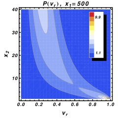
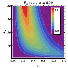
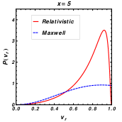
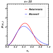
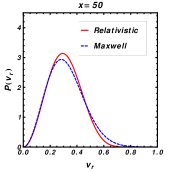
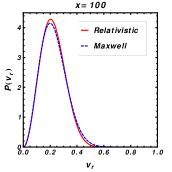
Figure 1: Top-left panel: contours of the relativistic distribution (17) in the plane $(V_{\texttt{r}}$, $x_{2}$). Top-right panel: contours of the Maxwell distribution (4). The parameter $x_{i}=m_{i}/T$ for the first particle is fixed to the non-relativistic value of $x_{1}=500$. Bottom panels: The relativistic distribution, Eq. (19), red lines, and the Maxwell distribution (4), blue lines, as a function of the relative velocity for increasing values of $x=m/T$. Here $m_{1}=m_{2}=m$.

(3) In the non-relativistic limit $V_{\text{r}}\sim v_{r}\ll 1$ and $x_{1,2}\gg 1$. It is useful to note the following relations between the parameters of the distribution:

$$\sqrt{2}X\sqrt{1+\varrho}=\frac{M}{T}=x_{1}+x_{2}\equiv\alpha,$$ (20)

$$\frac{X}{\sqrt{2}\sqrt{1+\varrho}}=\frac{\mu}{T}=\frac{x_{1}x_{2}}{x_{1}+x_{2}}\equiv\beta,$$ (21)

and that for $x\gg 1$ the asymptotic behavior of the modified Bessel function is $K_{n}(x)\sim e^{-x}\sqrt{{\pi}/{(2x)}}$. To the lowest order in $v^{2}_{r}$ and $X$ we have

$$\frac{X}{\sqrt{2}\prod_{i}K_{2}(x_{i})}\sim\frac{\sqrt{2}}{\pi}X^{2}e^{\alpha},$$ (22)

$$\gamma^{3}_{{}_{\texttt{r}}}\frac{\gamma^{2}_{{}_{\texttt{r}}}-1}{\sqrt{\gamma_{{\texttt{r}}}+\varrho}}\sim\frac{v^{2}_{r}}{\sqrt{1+\varrho}}=\sqrt{2}\frac{\beta}{X}{v^{2}_{r}},$$ (23)

$$K_{1}(\sqrt{2}X\sqrt{\gamma_{{\texttt{r}}}+\varrho})\sim\sqrt{\frac{\pi}{2}}\frac{\sqrt{\beta}}{X}e^{-\alpha}e^{-\beta\frac{v^{2}_{r}}{2}}.$$ (24)

Multiplying the Eqs. (22), (23), (24) we obtain the Maxwell distribution (4).

In actual calculations it is convenient to work with different variables rather than $V_{\texttt{r}}$. From Eq. (11) we can read the distribution as a function of $s$ and the respective diagonal form:

$$\begin{array}[]{l}\mathcal{P}_{\texttt{r}}(s)=\frac{1}{4T\prod_{i}m^{2}_{i}K_{2}(x_{i})}[s-(m^{2}_{1}+m^{2}_{2})]p^{\prime}K_{1}(\frac{\sqrt{s}}{T}),\end{array}$$ (26)

$$\begin{array}[]{l}\mathcal{P}^{d}_{\texttt{r}}(s)=\frac{1}{8Tm^{4}K^{2}_{2}(x)}(s-2m^{2})\sqrt{s-4m^{2}}K_{1}(\frac{\sqrt{s}}{T}).\end{array}$$ (28)

From Eq. (14) the distribution as function of $\gamma_{\texttt{r}}$ is

$$\begin{array}[]{l}\mathcal{P}_{\texttt{r}}(\gamma_{{}_{\texttt{r}}})=\frac{X}{\sqrt{2}\prod_{i}K_{2}(x_{i})}\gamma_{{}_{\texttt{r}}}\sqrt{\frac{\gamma^{2}_{{}_{\texttt{r}}}-1}{\gamma_{{}_{\texttt{r}}}+\varrho}}K_{1}(\sqrt{2}X\sqrt{\gamma_{{}_{\texttt{r}}}+\varrho}),\end{array}$$ (30)

$$\begin{array}[]{l}\mathcal{P}^{d}_{\texttt{r}}(\gamma_{\texttt{r}})=\frac{x}{\sqrt{2}K^{2}_{2}(x)}\gamma_{\texttt{r}}\sqrt{\gamma_{\texttt{r}}-1}K_{1}(\sqrt{2}x\sqrt{\gamma_{\texttt{r}}+1}).\end{array}$$ (32)

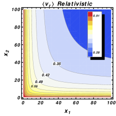
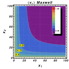
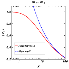
Figure 2: Left panel: contours of the mean value of the relativistic relative velocity, Eq. (39) in the plane ($x_{1}$, $x_{2}$). Central panel: contours in the same plane of the mean value of the relative velocity of the Maxwell distribution Eq. (40). Right panel: Eq. (41) as a function of $x=m/T$ , red line. The blue line is the Maxwell value (40) with $m_{1}=m_{2}=m$.

Both $\mathcal{P}_{\texttt{r}}(V_{\texttt{r}})$ and $F_{M}(v_{{r}})$ depend on the masses and the temperature through the ratios $x_{i}$ and are symmetric for the exchange $x_{1}\leftrightarrow x_{2}$. For a fixed temperature of the gas, when the masses are such that both $x_{1}$ and $x_{2}$ are much larger than 1, the Maxwell distribution is adequate. If this condition is not satisfied by one or both, then the relativistic distribution must be used. In Figure 1 we show the contours in the plane ($V_{\texttt{r}}$, $x_{2}$) of the relativistic distribution (17), left-top panel, and of the Maxwell distribution (4), right-top panel. We fix $x_{1}=500$ in the non-relativistic regime, and vary $x_{2}$ in the range (1, 40). The two distributions are very different in shape and absolute value. Note in particular that $\mathcal{P}_{\texttt{r}}(V_{\texttt{r}})$ has a large peak in the relativistic region $V_{\texttt{r}}\gtrsim 0.8$, $x\lesssim 5$. This peak is illustrated by plotting the relativistic $\mathcal{P}^{d}_{\texttt{r}}(V_{\texttt{r}})$, Eq. (19), and Maxwell distribution with $\mu=m/2$ at $x=5$, first of the bottom panels of Figure 1 where we study the case $m_{1}=m_{2}=m$. At small $x$ the distributions largely differ and become practically equal at $x\sim 100$.

III Mean value of the relative velocity

An important quantity that characterizes the p.d.f. is the mean value of the relative velocity,

$$\langle V_{\texttt{r}}\rangle=\int_{0}^{1}dV_{\texttt{r}}\mathcal{P}_{\texttt{r}}(V_{\texttt{r}})V_{\texttt{r}}.$$ (33)

It is convenient to use $\mathcal{P}_{\texttt{r}}(\gamma_{\texttt{r}})$, Eq. (30) and $V_{\texttt{r}}=\sqrt{\gamma^{2}_{\texttt{r}}-1}/\gamma_{\texttt{r}}$. The integral in Eq. (33) then becomes

$$\langle V_{\texttt{r}}\rangle=\frac{X}{\sqrt{2}\prod_{i}K_{2}(x_{i})}\int_{1}^{\infty}d\gamma_{{}_{\texttt{r}}}\frac{\gamma^{2}_{{}_{\texttt{r}}}-1}{\sqrt{\gamma_{{}_{\texttt{r}}}+\varrho}}K_{1}(\sqrt{2}X\sqrt{\gamma_{\texttt{r}}+\varrho}).$$

We change variable to $y=(\gamma_{\texttt{r}}+\varrho)/(1+\varrho)$ and define

$$c_{2}=(1+\varrho)^{2},\;\;c_{1}=2\varrho(1+\varrho),\;\;c_{0}=\varrho^{2}-1.$$ (34)

Using Eq. (20) and (34), after some algebra, we find

$$\langle V_{\texttt{r}}\rangle=\frac{\alpha}{2\prod_{i}K_{2}(x_{i})}(c_{2}\mathcal{I}_{2}-c_{1}\mathcal{I}_{1}+c_{0}\mathcal{I}_{0}),$$ (35)

where the integrals

$$\mathcal{I}_{2}=\int_{1}^{\infty}dy\,y^{\frac{3}{2}}K_{1}(\alpha\sqrt{y})=\frac{2}{\alpha}K_{2}(\alpha)+\frac{4}{\alpha^{2}}K_{3}(\alpha),$$ (36)

$$\mathcal{I}_{1}=\int_{1}^{\infty}dy\,y^{\frac{1}{2}}K_{1}(\alpha\sqrt{y})=\frac{2}{\alpha}K_{2}(\alpha),$$ (37)

$$\mathcal{I}_{0}=\int_{1}^{\infty}dy\,y^{-\frac{1}{2}}K_{1}(\alpha\sqrt{y})=\frac{2}{\alpha}K_{0}(\alpha),$$ (38)

are calculated in the Appendix.

Using the recursion formulas of the Bessel functions we finally find

$$\langle V_{\texttt{r}}\rangle=\frac{2}{\alpha}\frac{c_{2}K_{3}(\alpha)-c_{0}K_{1}(\alpha)}{K_{2}(x_{1})K_{2}(x_{2})}.$$ (39)

In the non-relativistic limit it gives the Maxwell’s value

$$\langle v_{r}\rangle=\sqrt{\frac{8T}{\pi\mu}}=\sqrt{\frac{8}{\pi}}\sqrt{\frac{x_{1}+x_{2}}{x_{1}x_{2}}}.$$ (40)

It is easier to study the limit in the case $m_{1}=m_{2}=m$, the diagonal of the plane ($x_{1}$, $x_{2}$). We have $\alpha=2x$, $c_{2}=4$, $c_{0}=0$, thus formula (39) simplifies to

$$\langle V_{\texttt{r}}\rangle_{d}=\frac{4}{x}\frac{K_{3}(2x)}{K^{2}_{2}(x)}.$$ (41)

Using the asymptotic expansions of $K_{n}(x)$ for $x\gg 1$ we find the non-relativistic expansion,

$$\langle V_{\texttt{r}}\rangle_{d}\sim 4\sqrt{\frac{1}{\pi x}}\left[1-\frac{25}{16}\frac{1}{x}+\frac{1305}{512}\frac{1}{x^{2}}+\mathcal{O}(x^{-3})\right].$$ (42)

To the lowest order coincides with the Maxwell value $\langle v_{{r}}\rangle_{d}=4\sqrt{{1}/{(\pi x)}}$ as expected. In the ultra-relativistic limit, $x\ll 1$, we find

$$\langle V_{\texttt{r}}\rangle_{d}\sim 1+\mathcal{O}(x^{4}),$$ (43)

thus $\langle V_{\texttt{r}}\rangle$ tends to the velocity of light.

In the left panel of Fig. (2) we show the contours of the mean value (39) in the plane ($x_{1}$, $x_{2}$). At small $x$ it tends to 1 in both the ”directions” $x_{1}$, $x_{2}$. In the central panel we show the contours of the Maxwell’s value (40). At $x_{i}<40$ the two mean values starts to differ significantly, and obviously the latter does not respect the constraint $\langle v_{r}\rangle\leq 1$. In the right panel of Fig. 2 we plot Eq. (41). At $x\lesssim 0.7$, $\langle V_{\texttt{r}}\rangle$ is already well approximated by the asymptotic value 1. In fact, as indicated by (43), the first corrections to 1 is of the order $\mathcal{O}(x^{4})$, thus very small. We find that the first three terms of the asymptotic expansion in Eq. (42) approximate well the exact function for $x\gtrsim 5$. The non-relativistic Maxwell value $\langle v_{{r}}\rangle=4\sqrt{{1}/{\pi x}}$ is always greater than the relativistic value $\langle V_{\texttt{r}}\rangle$ and it is a good approximation for $x>40$.

IV Summary and final remarks

Guided by the principles of special relativity, Lorentz invariance and by the Jüttner distribution, we have found the probability distribution $\mathcal{P}_{\texttt{r}}(V_{\texttt{r}})$ of the relativistic relative velocity of binary collisions in a relativistic non-degenerate gas, Eq. (17), and an exact formula for the mean value of the relative velocity, Eq. (39). When at least one particle is relativistic, the Maxwell distribution is inadequate. Whenever a relativistic treatment is necessary, the non-relativistic unit rate or thermal averaged cross section $\langle\sigma v_{r}\rangle=\int_{0}^{\infty}dv_{r}F_{M}(v_{r})\sigma v_{r}$ can be replaced by the relativistic analogous $\langle\sigma V_{\texttt{r}}\rangle=\int_{0}^{1}dV_{\texttt{r}}\mathcal{P}_{\texttt{r}}(V_{\texttt{r}})\sigma V_{\texttt{r}}$.

It is worth noting that a crucial step to derive the distribution is to not introduce, as usually done Landau2 ; Cercignani ; DeGroot , the so called Møller velocity $\bar{v}={(1-\boldsymbol{v}_{1}\cdot\boldsymbol{v}_{2})}{{V}_{\texttt{r}}}=\frac{p_{1}\cdot p_{2}}{E_{1}E_{2}}{V}_{\texttt{r}}$, but to maintain the factor $p_{1}\cdot p_{2}/(E_{1}E_{2})$ that guarantees the invariance of the product $n_{1}n_{2}(p_{1}\cdot p_{2})/(E_{1}E_{2})$ explicitly in the integral (9).

One consequence of the present findings regards the thermal averaged cross section that appear in the calculation of the dark matter relic density. After Ref. GG , it was accepted that in a relativistic framework, the velocity in $\langle\sigma{v}\rangle$ is the Møller velocity and for this reason often written in literature as ”relative velocity”. The Møller velocity is not a fundamental quantity but it is derived from the relativistic relative velocity. We fully discuss this point in a separate work paperSV .

Appendix A Integrals involving modified Bessel functions

The integrals involved in the calculation of the mean relative velocity can be reduced to the known integrals GR

$$\int_{1}^{\infty}dzz^{\lambda}(z-1)^{\mu-1}K_{\nu}(a\sqrt{z})=$$

$$\;\;\;\;\Gamma(\mu)2^{2\lambda-1}a^{-2\lambda}G_{1,3}^{3,0}\begin{pmatrix}\frac{a^{2}}{4}\Biggr{\rvert}\begin{array}[]{c}0\\ -\mu,\frac{\nu}{2}+\lambda,-\frac{\nu}{2}+\lambda,\end{array}\end{pmatrix},$$ (44)

$$\int_{1}^{\infty}dzz^{-\frac{\nu}{2}}(z-1)^{\mu-1}K_{\nu}(a\sqrt{z})=\Gamma(\mu)2^{\mu}a^{-\mu}K_{\nu-\mu}(a),$$ (45)

where $G^{m,n}_{p,q}(x|\{a_{1},...,a_{n},...,a_{p}\},\{b_{1},...,b_{m},...,b_{q}\})$ is the generalized hypergeometric Meijer’s $G$ function GR . When one of the upper indexes is equal to one of the lower indexes the function is reduced to a simpler $G$ function, for example if $a_{p}=b_{q}=c$,

$$G^{m,n}_{p,q}\left(z\Bigg{\rvert}\begin{matrix}{}a_{1},...,c\\ b_{1},...,c\end{matrix}\right)=G^{m-1,n}_{p-1,q-1}\left(z\Bigg{\rvert}\begin{matrix}{}a_{1},...,a_{p-1}\\ b_{1},...,b_{q-1}\end{matrix}\right).$$ (46)

The the modified Bessel functions are a particular $G$ function:

$$G_{0,2}^{2,0}\left(\frac{z^{2}}{4}\Bigg{\rvert}\begin{array}[]{c}\\ \frac{\delta+\nu}{2},\frac{\delta-\nu}{2}\end{array}\right)=\frac{z^{\delta}}{2^{\delta-1}}K_{\nu}(z).$$ (49)

Using the property (46) we see that (45) is a particular case of Eq. (44) with $\lambda=-\nu/2$.

The integral $\mathcal{I}_{0}$, Eq. (38), follows directly form Eq. (45) with $\nu=\mu=1$. The integral $\mathcal{I}_{1}$, Eq. (37), follows from Eq. (44) with $\lambda=1/2$, $\mu=1$, $\nu=1$ and reducing the resulting $G$ function with the property (46). To calculate $\mathcal{I}_{2}$, Eq. (36), we first note that Eq. (44) with $\lambda=1/2$, $\mu=2$, $\nu=1$ gives

$$\mathcal{J} =\int_{1}^{\infty}dzz^{\frac{1}{2}}(z-1)K_{1}(a\sqrt{z})=\frac{1}{a}G_{1,3}^{3,0}\begin{pmatrix}\frac{a^{2}}{4}\Biggr{\rvert}\begin{array}[]{c}0\\ -2,1,0\end{array}\end{pmatrix}$$ (50)

$$=\frac{1}{a}G_{0,2}^{2,0}\begin{pmatrix}\frac{a^{2}}{4}\Biggr{\rvert}\begin{array}[]{c}\\ -2,1\end{array}\end{pmatrix}=\frac{4}{a^{2}}K_{3}(a),$$ (51)

where we used (46). Finally, $\mathcal{J}+\mathcal{I}_{1}=\mathcal{I}_{2}$ that gives (36).