Weak lensing with 21 cm intensity mapping at $z\sim 2-3$

Abstract

We study how 21 cm intensity mapping can be used to measure gravitational lensing over a wide range of redshift. This can extend weak lensing measurements to higher redshifts than are accessible with conventional galaxy surveys. We construct a convergence estimator taking into account the discreteness of galaxies and calculate the expected noise level as a function of redshift and telescope parameters. At $z\sim 2-3$ we find that a telescope array with a collecting area $\sim 0.2\,{\rm km}^{2}$ spread over a region with diameter $\sim 2\,{\rm km}$ would be sufficient to measure the convergence power spectrum to high accuracy for multipoles between 10 and 1,000. We show that these measurements can be used to constrain interacting dark energy models.

1 Introduction

We now live in an era of precision cosmology. Almost all of the information used to achieve this precision has come from redshifts below $z\sim~{}1.5$ or from the Cosmic Microwave Background (CMB) at $z\sim 1000$. The vast regions between these redshifts have been probed only sparsely. Given our ignorance of what is causing the apparent acceleration of the Universe, it is important that we explore the evolution of expansion and structure formation over the widest possible range of redshift. It is possible that dark energy, or a modification to general relativity, came into play at higher redshift than the standard cosmological constant model predicts (Copeland, Sami & Tsujikawa, 1006; Clifton et al., 2012). Early dark energy models are an example of this. In recent years, several 21 cm surveys have been proposed to study the epoch of reionization (EoR) which could provide some cosmological information at $z\sim 8-12$. The gravitational lensing of the CMB also provides some information on the intermediate redshifts, but the signal-to-noise is low. The clustering of quasars and Ly-$\alpha$ absorption lines in quasar spectra can be measured at high redshift, but here bias and modeling uncertainties are serious problems. In this paper we address the prospects for measuring gravitational lensing at redshifts after reionization, but before those probed by galaxy surveys in the visible bands.

In Zahn & Zaldarriaga (2005) and Metcalf & White (2009) it was shown that if the EoR is at redshift $z\sim 8$ or later, a large radio telescope such as SKA (Square Kilometer Array) could measure the lensing convergence power spectrum and constrain the standard cosmological parameters. The authors extended the Fourier-space quadratic estimator technique, which was first developed by (Hu, 2001) for CMB lensing observations to three dimensional observables, i.e. the $21$ cm intensity field $I(\theta,z)$. These studies did not consider 21 cm observations from redshifts after reionization when the average HI density in the universe is much smaller.

It has also been proposed that lensing could be measured at lower redshifts by counting the fluctuations in the number density of detected 21 cm objects on the sky as a measure of the magnification (Zhang & Pen, 2005, 2006; Zhang & Yang, 2011). The signal-to-noise is greatly reduced in this case because of the low number density of objects and the intrinsic clustering of them.

Lensing surveys in the visible are limited in redshift by the number density of detected galaxies with measurable ellipticities. This is strongly dependent on the depth of the survey, but any proposed survey that will cover a significant fraction of the sky will be quite sparse in sources above $z\sim 1.5$. Here we show that 21 cm observations can be used to extend weak lensing measurements to higher redshifts than this, but still well below the redshift of reionization or the CMB.

21 cm intensity mapping is a technique that has been proposed for measuring the distribution of HI gas before and during reionization (see Furlanetto et al. (2006) for a review) and measuring the BAO at redshifts of order unity (Chang et al., 2008, 2010; Seo et al., 2010; Masui et al., 2010; Ansari et al., 2012; Battye et al., 2012; Chen, 2012; Pober et al., 2013). In this technique, no attempt is made to detect individual objects. Instead the 21 cm emission is treated as a continuous three dimensional field. The angular resolution of the telescope need not be high enough to resolve individual galaxies which makes observations at high redshift possible with a reasonably sized telescope. Foregrounds are expected to have smoother spectra than the signal so they can be subtracted by filtering in frequency.

In this study, we extend the 21 cm lensing method further, taking into account the discreteness of galaxies. In Section 2, we present our formalism for constructing a lensing estimator and calculating the corresponding lensing reconstruction noise. In Section 3, we investigate the possibility of measuring lensing at intermediate redshifts and show results using telescope arrays optimized for high signal-to-noise. Measurements of the convergence power spectrum can be used to constrain interacting dark energy models. We conclude in Section 4.

2 Formalism

The mean observed brightness temperature at redshift $z$ due to the average HI density can be written as (Battye et al., 2012)

$$\bar{T}(z)=180\;\Omega_{\rm HI}(z)\;h\frac{(1+z)^{2}}{E(z)}\;{\rm mK},$$ (1)

where the Hubble parameter $h=H_{0}/100\,{\rm km}\,{\rm s}^{-1}\,{\rm Mpc}^{-1}$, $E(z)=H(z)/H_{0}$ and $\Omega_{\rm HI}(z)=8\pi G\rho_{\rm HI}(z)/(3H^{2}_{0})$ is the average HI density at redshift $z$ relative to the present day critical density. Consequently, the 3D HI power spectrum of the brightness temperature fluctuations is given by

$$P_{\Delta T_{b}}(k)=[\bar{T}(z)]^{2}(1+f\mu^{2}_{k})^{2}P_{\delta}(k),$$ (2)

where $P_{\delta}(k)$ is the underlying dark matter power spectrum, $f=\frac{d\ln D}{d\ln a}\simeq\Omega_{m}(z)^{0.55}$ where $D$ is the linear growth rate and $\mu_{k}$ is the cosine of the angle between the wave vector ${\bf k}$ and the line of sight $\hat{z}$. The scale parameter is $a=(1+z)^{-1}$.

In Zahn & Zaldarriaga (2005) and Metcalf & White (2009) the convergence estimator and the corresponding lensing reconstruction noise are calculated assuming that the temperature (brightness) distribution is Gaussian. The advantage of 21cm lensing is that one is able to combine information from multiple redshift slices. In Fourier space, the temperature fluctuations are divided into perpendicular to the line of sight wave vectors $\mathbf{k_{\perp}}=\mathbf{l}/{\cal D}$, with ${\cal D}$ the angular diameter distance to the source redshift, and a discretized version of the parallel wave vector $k_{\parallel}=\frac{2\pi}{{\cal L}}j$ where ${\cal L}$ is the depth of the observed volume. Considering modes with different $j$ independent, an optimal estimator can be found by combining the individual estimators for different $j$ modes without mixing them. The three-dimensional lensing reconstruction noise is then found to be (Zahn & Zaldarriaga, 2005)

$$N(\mathbf{L})=\left[\sum_{j}^{j_{\rm max}}\frac{1}{L^{2}}\int\frac{d^{2}\ell}{(2\pi)^{2}}\frac{[\mathbf{l}\cdot\mathbf{L}C_{\ell,j}+\mathbf{L}\cdot(\mathbf{L}-{\bf l})C_{|\ell-L|,j}]^{2}}{2C^{\rm tot}_{\ell,j}C^{\rm tot}_{|{\bf l}-\mathbf{L}|,j}}\right]^{-1},$$ (3)

where

$$C_{\ell,j}=\frac{P_{\Delta T_{b}}(\sqrt{(\ell/{\cal D})^{2}+(j2\pi/{\cal L})^{2}})}{{\cal D}^{2}{\cal L}}=[\bar{T}(z)]^{2}P_{\ell,j}.$$ (4)

However, the Gaussian case is an approximation which breaks down if we take into account the discreteness of galaxies in the Universe. After reionization, the HI resides mostly in the galaxies. A more realistic model the HI distribution, and the one most often assumed, is a Poisson distribution drawn from a Gaussian distribution representing the clustering of galaxies. In order to calculate a lensing estimator and the corresponding lensing reconstruction noise for this model, we will work with the discrete Fourier transform of the intensity field $I(\mathbf{x})$, which we write as

$$I_{{\bf k}}=\frac{\Omega_{s}}{N_{\perp}N_{\parallel}}\sum_{\mathbf{x}}e^{i{\bf k}\cdot\mathbf{x}}I(\mathbf{x}),$$ (5)

where ${\bf k}=(\mathbf{l},j)$, $\mathbf{x}=(\theta,z)$ and $\Omega_{s}=\Theta_{s}\times\Theta_{s}$ for a square survey geometry. $N_{\perp}$ and $N_{\parallel}$ are the number of cells in the volume perpendicular and paralel to the radial direction. We also have

$$I(\mathbf{x})=\frac{1}{\Omega_{s}}\sum_{{\bf k}}e^{-i{\bf k}\cdot\mathbf{x}}I_{{\bf k}}.$$ (6)

For the $2$-point correlation function we get

$$<I(\mathbf{x})I(\mathbf{x}^{\prime})>=\frac{1}{\bar{\eta}\delta V}\frac{<M^{2}>}{<M>^{2}}\delta^{K}_{\mathbf{x}\mathbf{x}^{\prime}}+\xi_{\mathbf{x}\mathbf{x}^{\prime}}.$$ (7)

Fourier transforming we find

$$<I_{{\bf k}}I^{*}_{{\bf k}^{\prime}}>=\Omega_{s}\;(P_{\ell,j}+P^{\rm shot})\;\delta^{K}_{\ell,\ell^{\prime}}\delta^{K}_{jj^{\prime}},$$ (8)

where $P_{\ell,j}$ is given by Equation (4) and

$$P^{\rm shot}=\frac{1}{\bar{\eta}}\frac{1}{D^{2}{\cal L}}\frac{<M^{2}>}{<M>^{2}},$$ (9)

with $\bar{\eta}$ the average number density of galaxies and the $M$ moments must be computed from an appropriate mass (or luminosity) function. The lensing correlation gives

$$<\tilde{I}_{\mathbf{l},j}\tilde{I}^{*}_{\mathbf{l}-\mathbf{L},j^{\prime}}>=\delta^{K}_{jj^{\prime}}\times$$

$$[\mathbf{l}\cdot\mathbf{L}P_{\ell,j}+\mathbf{L}\cdot(\mathbf{L}-{\bf l})P_{|\ell-L|,j}+L^{2}\;P^{\rm shot}]\;\Psi(\mathbf{L}).$$ (10)

We can construct a lensing estimator of the form

$$\hat{\Psi}(\mathbf{L})=f(\mathbf{L})\sum_{j}^{j_{\rm max}}\sum_{\mathbf{l}}\tilde{I}_{\mathbf{l},j}\tilde{I}^{*}_{\mathbf{l}-\mathbf{L},j},$$ (11)

where $f(\mathbf{L})$ is a normalization. In order for the estimator to be unbiased we impose

$$<\hat{\Psi}(\mathbf{L})>=\Psi(\mathbf{L}),$$ (12)

and we find (note $P_{\ell,j}\rightarrow C_{\ell,j}$ from now on, as in Eq. (4))

$$f(\mathbf{L})=\bigg{\{}\sum_{j}^{j_{\rm max}}\sum_{\mathbf{l}}[\mathbf{l}\cdot\mathbf{L}C_{\ell,j}+\mathbf{L}\cdot(\mathbf{L}-{\bf l})C_{|\ell-L|,j}+L^{2}\;C^{\rm shot}]\bigg{\}}^{-1},$$ (13)

with $C^{\rm shot}=[\bar{T}(z)]^{2}P^{\rm shot}$.

We are now ready to compute the lensing reconstruction noise $N(L)$, which corresponds to the variance of the estimator ${\cal V}=<\hat{\Psi}(\mathbf{L})\hat{\Psi}^{\star}(\mathbf{L})>$. After some algebra and using

$$\sum_{\mathbf{l}}\rightarrow\Omega_{s}\int\frac{d^{2}\ell}{(2\pi)^{2}}$$

to move from discrete to continuous $\ell$-space we find

$$N(L)=L^{2}\times$$

$$\frac{{\cal N}_{0}+{\cal N}_{1}+{\cal N}_{2}+{\cal N}_{3}+{\cal N}_{4}}{\bigg{\{}\displaystyle\sum_{j}^{j_{\rm max}}\int\frac{d^{2}\ell}{(2\pi)^{2}}[\mathbf{l}\cdot\mathbf{L}C_{\ell,j}+\mathbf{L}\cdot(\mathbf{L}-{\bf l})C_{|\ell-L|,j}+L^{2}\;C^{\rm shot}]\bigg{\}}^{2}}\,,$$ (14)

with

$${\cal N}_{0}=[\bar{T}(z)]^{4}(j_{\rm max})^{2}\frac{1}{\bar{\eta}^{3}}\frac{1}{(D^{2}{\cal L})^{3}}\frac{<M^{4}>}{<M>^{4}}\left(\int\frac{d^{2}\ell}{(2\pi)^{2}}\right)^{2},$$

$${\cal N}_{1}=[\bar{T}(z)]^{2} (j_{\rm max})\frac{1}{\bar{\eta}^{2}}\frac{1}{(D^{2}{\cal L})^{2}}\frac{<M^{3}>}{<M>^{3}}\left(\int\frac{d^{2}\ell^{\prime}}{(2\pi)^{2}}\right)$$

$$\times\sum_{j}^{j_{\rm max}}\int\frac{d^{2}\ell}{(2\pi)^{2}}[2C^{\rm tot}_{\ell,j}+2C^{\rm tot}_{|\ell-L|,j}],$$

$${\cal N}_{2}=[\bar{T}(z)]^{2} \frac{1}{\bar{\eta}^{2}}\frac{1}{(D^{2}{\cal L})^{2}}\frac{<M^{2}>^{2}}{<M>^{4}}\sum_{j}^{j_{\rm max}}\sum_{j^{\prime}}^{j_{\rm max}}\int\frac{d^{2}\ell}{(2\pi)^{2}}\int\frac{d^{2}\ell^{\prime}}{(2\pi)^{2}}$$

$$\;\;\;\;\;\;\;\;\;\;\;\;\;\;\;\;\;\;\;\;\;\;\times[C^{\rm tot}_{|\ell-\ell^{\prime}|,|j-j^{\prime}|}+C^{\rm tot}_{|\ell+\ell^{\prime}-L|,j+j^{\prime}}],$$

$${\cal N}_{3} =C^{\rm shot}\sum_{j}^{j_{\rm max}}\int\frac{d^{2}\ell}{(2\pi)^{2}}[2C^{\rm tot}_{\ell,j}+2C^{\rm tot}_{|\ell-L|,j}]$$

and

$${\cal N}_{4} =\int\frac{d^{2}\ell}{(2\pi)^{2}}2C^{\rm tot}_{\ell,j}C^{\rm tot}_{|\ell-L|,j}\,,$$

where $C^{\rm tot}_{\ell,j}=C_{\ell,j}+C^{\rm N}_{\ell}$, with $C^{\rm N}_{\ell}$ the thermal noise of the telescope.

In the next section, we will use the constructed estimator and noise to investigate how well the convergence power spectrum can be measured from data as a function of telescope parameters. Note that the derived noise contains the HI mass moments (up to 4th order), which need to be calculated assuming an adequate mass function. The most interesting feature of Eq. (14) is that the shot noise terms contribute to both the noise and the signal in the lensing measurement.

A significant difficulty in 21 cm experiments is foreground contamination from galactic synchrotron, point sources, bremsstrahlung etc. These foreground contributions are smooth power laws in frequency, and it is expected that they can be removed to high accuracy. We will present a study of foreground removal in a future paper. For now, we note that foreground removal will make the first few $j$-modes useless for the reconstruction (Zahn & Zaldarriaga, 2005), so we have discarded the $j=0$ mode in our calculations.

3 Results

In general, there are three main epochs of interest: (i) the Dark Ages before reionization, where the HI fraction is high but so are the foregrounds and noise (ii) the EoR (iii) the epoch after reionization. During the latter epoch, the HI fraction is much lower ($\sim 1\%$ today), but the foregrounds and noise are also lower.

For this work we will concentrate on the last epoch and work at a redshift $z_{s}=2$, which corresponds to a frequency $\nu=473\,\rm{MHz}$ (detailed work on all three epochs will be presented in a future paper). Considering a uniform distribution ground based array of telescopes, the power spectrum of the thermal noise will be

$$C^{\rm N}_{\ell}=\frac{(2\pi)^{3}T^{2}_{\rm sys}}{Bt_{\rm obs}f^{2}_{\rm cover}\ell_{\rm max}(\nu)^{2}}\,,$$ (15)

where $T_{\rm sys}$ is the system temperature, $B$ is the bandwidth, $t_{\rm obs}$ the total observation time, $D_{\rm tel}$ the diameter of the array and $\ell_{\rm max}(\lambda)=2\pi D_{\rm tel}/\lambda$ is the highest multipole that can be measured by the array at frequency $\nu$ (wavelength $\lambda$). $f_{\rm cover}$ is the total collecting area of the telescopes $A_{\rm coll}$ divided by $\pi(D_{\rm tel}/2)^{2}$, the aperture covering fraction. Our chosen telescope configuration follows a SKA-like design. The total collecting area is $\sim 0.19\;{\rm km}^{2}$ (30% of the full SKA) and the maximum baseline is $D_{\rm tel}=2\;{\rm km}$, giving an $f_{\rm cover}\simeq 0.06$ and a value of $\ell_{\rm max}\sim 19900$. We consider a $2\,{\rm yr}$ observation time and a $40\,{\rm MHz}$ bandwidth. Note that the change of the convergence power spectrum across the corresponding redshift interval is very small. This would not be the case at a much higher redshift (e.g. $z\sim 8$), where we would have to use smaller bandwidths $\sim 1\,{\rm MHz}$.

The most important source of noise is Galactic synchrotron emission, approximated by

$$T_{\rm syn}=180\;{\rm K}\;(\nu/180\;{\rm MHz})^{-2.6}.$$ (16)

However, at $z=2$ this is subdominant in comparison to the receiver temperatures which we estimate to be $\sim 50\,{\rm K}$, and this is the value we are going to use for $T_{\rm sys}$.

In order to calculate the Poisson terms we need the HI mass function. The comoving number density of galaxies $dn$ in a mass range $dM$ is taken to be a Schechter function

$$\frac{dn}{dM}dM=\phi^{\star}\left(\frac{M}{M^{\star}}\right)^{\alpha}{\rm exp}\left[-\frac{M}{M^{\star}}\right]\frac{dM}{M^{\star}},$$ (17)

parametrized by a low-mass slope $\alpha$, a characteristic mass $M^{\star}$ and a normalization $\phi^{\star}$. We can calculate $\rho_{\rm HI}$ using

$$\rho_{\rm HI} =\phi^{\star}M^{\star}\int\left(\frac{M}{M^{\star}}\right)^{\alpha+1}{\rm exp}\left[-\frac{M}{M^{\star}}\right]\frac{dM}{M^{\star}}$$

$$=\phi^{\star}M^{\star}\;\Gamma(\alpha+2),$$ (18)

where $\Gamma$ denotes the Gamma function. The HI mass density relative to the critical density of the Universe $\rho_{\rm c}=2.7755\,h^{2}10^{11}\,M_{\odot}\,{\rm Mpc}^{-3}$ is

$$\Omega_{\rm HI}=\frac{\rho_{\rm HI}}{\rho_{\rm c}}=\frac{\phi^{\star}M^{\star}\;\Gamma(\alpha+2)}{\rho_{\rm c}},$$ (19)

and is used in Equation (1) to calculate $\bar{T}(z)$.

The parameters ($\alpha,M^{\star},\phi^{\star}$) are the most important source of systematic uncertainty in our study. They are only well measured in the local Universe. We assume a no-evolution model using the values $\alpha=-1.3,M^{\star}=3.47h^{-2}10^{9}\,M_{\odot},\phi^{\star}=0.0204\,h^{3}\,{\rm Mpc}^{-3}$ reported from the HIPASS survey (Zwaan et al., 2003). Other models derived from Lyman-$\alpha$ systems are possible (see, for example, (Peroux et al., 2003)), but we feel that no-evolution is a conservative choice.

One of the first objectives of a $21\rm{cm}$ lensing survey will be to measure the two-point statistics of the convergence field $\kappa(\vec{L},z_{s})$ or, equivalently, the displacement field $\delta\theta(\vec{L},z_{s})$, averaged over $z_{s}$. That is,

$$C_{L}^{\delta\theta\delta\theta}=\frac{9\Omega^{2}_{m}H^{3}_{0}}{L(L+1)c^{3}}\int_{0}^{z_{s}}dz\,P_{\delta}(k=L/{\cal D}(z),z)[W(z)]^{2}/E(z),$$ (20)

where $W(z)=({\cal D}(z_{s})-{\cal D}(z))/{\cal D}(z_{s})$. The expected error in the power spectrum $C_{L}^{\delta\theta\delta\theta}$ averaging over $\mathbf{L}$ directions in a band of width $\Delta L$ is given by

$$\Delta C_{L}^{\delta\theta\delta\theta}=\sqrt{\frac{2}{(2L+1)\Delta Lf_{\rm{sky}}}}\left(C_{L}^{\delta\theta\delta\theta}+N_{L}\right).$$ (21)

There is a limit to the number of $j$-modes that can be used in $N_{L}$. For very high $j$ the internal velocity structure of galaxies will be resolved and our statistical model which treats them as point sources will break down. To find the maximum $j$, we use the formula $\Delta v/c=B/f$ to calculate the velocity width corresponding to our chosen bandwidth $B$ at the observed frequency $f$, and then we divide with a typical velocity dispersion for a galaxy at $z=2$ ($f=473\,{\rm MHz}$), which we assume to be $200\,{\rm km/s}$. This gives $j_{\rm max}=126$, but the noise has already converged at $j\sim 40$.

In Fig. 1 we compare the signal (solid black line), i.e. the displacement field power spectrum $C_{L}^{\delta\theta\delta\theta}$, with the noise $N_{L}$ (dashed black line). As in the Gaussian case, the shape of $L^{2}N_{L}$ approaches a constant — it does diverge in very high multipoles due to the thermal noise. The measured lensing power spectrum will also depend on the multipole binning $\Delta L$ and the fraction of the sky surveyed $f_{\rm sky}$, as shown from Eq. (21). Choosing $f_{\rm sky}=0.2$ and $\Delta L=36$ we get the measurement errors shown in Fig. 1. Repeating the calculation assuming the sources are at redshift $z_{s}=3$, we get the results shown in Fig. 1 for the signal $C_{L}^{\delta\theta\delta\theta}$ (dot-dashed magenta line) and the noise $N_{L}$ (dotted magenta line).

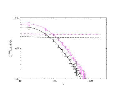
Figure 1: Displacement field power spectrum (solid black line) and lensing reconstruction noise $N_{L}$ (dashed black line, equation (14)) for the compact SKA-like telescope described in the text, at redshift $z=2$. $N_{L}$ converges well before $j$ reaches a reasonable $j_{\rm max}$, making the results insensitive to the exact value of this parameter. The measurement errors come from sample variance and $N_{L}$ according to Eq. (21). We have chosen $f_{\rm sky}=0.2$ and $\Delta L=36$. Note that the signal can be probed up to a much lower value than $\ell_{\rm max}\sim 19900$, the highest multipole the telescope can reach. We also show the results for redshift $z=3$ (dot-dashed and dotted magenta lines).

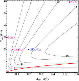
Figure 2: The signal-to-noise (21) at $L=100$ for various telescope configurations. Sources are at $z=2$. The contour lines are labelled with the $(S/N)$ values. The area under the red solid line is excluded, since it corresponds to $f_{\rm cover}>1$. Some telescopes are shown for comparison although MWA and LOFAR do not operate at the required frequency for this experiment.

In Fig. 2 we show the signal-to-noise (S/N) values at multipole $L=100$ spanning the parameter space $(D_{\rm max},A_{\rm coll})$. A LOFAR-like telescope could in principle give good results, but it does not operate at the right frequencies to observe at $z=2$. The sparse SKA core array with $D_{\rm max}=6\,{\rm km}$ gives a high S/N value at $L=100$, but the more compact SKA-like configuration we have chosen performs better when one computes the total noise (i.e. taking into account the contributions at all $L$), due to its higher covering fraction.

Measurements of the weak lensing signal, such as those presented in Fig. 1, can be used to constrain interactions in the dark sector. To illustrate this point we will adopt several concrete dark energy models. Pourtsidou, Skordis & Copeland (2013) found three distinct classes of dark energy models in the form of a scalar field $\phi$ coupled to cold dark matter (subscript cdm). The first two types involve energy and momentum transfer between the dark sectors, while the third is a pure momentum transfer model. The coupled quintessence (CQ) model suggested by Amendola (2000) belongs to the Type-1 class. In such a model, the Bianchi identities can be written as

$$\nabla_{\nu}T^{\nu}_{(\phi)\mu}=-J_{\mu}=-\nabla_{\nu}T^{\nu}_{({\rm cdm})\mu},$$ (22)

so that the total energy-momentum tensor of the dark sector is conserved. The CQ Type-1 model has a coupling current

$$J_{\mu}=-\alpha_{0}\rho_{\rm cdm}\nabla_{\mu}\phi,$$ (23)

where $\alpha_{0}$ is a constant coupling parameter and $\rho_{\rm cdm}=\rho_{\rm cdm,0}a^{-3}e^{\alpha_{0}\phi}$ is the CDM density for this model. We also consider a single exponential potential $V(\phi)$ for the quintessence field. Using a modified version of the CAMB code (Lewis, Challinor & Lasenby, 2000) we can study the background cosmology and the linear perturbations of the chosen model (for details, see Pourtsidou, Skordis & Copeland, 2013). We construct the displacement field power spectrum and compare it with the $\Lambda$CDM prediction in Fig. 1. Note that each cosmology evolves to the PLANCK cosmological parameter values (Ade et al., 2013). As we can see in Fig. 3, the Type-1 model with a coupling parameter $\alpha_{0}=0.1$ would be excluded. Here there is energy transfer from dark matter to dark energy making the dark matter density larger in the past compared to the non-interacting case for fixed $\Omega_{m}$ today, hence the gravitational potential is higher and the convergence power spectrum is enhanced. The Type-3 class of models in (Pourtsidou, Skordis & Copeland, 2013) is particularly interesting, as the background energy densities evolve as in the uncoupled case. More specifically, in Type-3 models no coupling appears in the fluid equations at the background level. Furthermore, the energy-conservation equation remains uncoupled also at the linear level, so we have a pure momentum-transfer coupling at the level of linear perturbations. Working with the CQ Type-3 case studied in (Pourtsidou, Skordis & Copeland, 2013), we find that the lensing signal is suppressed and a model with coupling parameter $\gamma_{0}=0.2$ would be excluded (see Fig. 3).

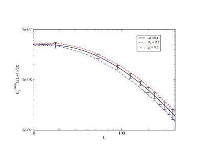
Figure 3: Displacement field power spectrum for $\Lambda$CDM compared with two different interacting dark energy models. Sources are at $z=2$. The error bars are the same as in figure 1.

4 Discussion and conclusions

Past work has been more pessimistic on the prospects of measuring lensing from 21 cm radiation at the redshifts discussed here (Zhang & Pen, 2005, 2006; Zhang & Yang, 2011). We believe that this is because those studies were based on counting the number of galaxies that are several sigma above the noise. With that approach the clustering of galaxies and the shot noise from their discreteness contribute purely to noise in the lensing estimator. In our approach, shot noise and clustering contribute to both the noise and to an improvement in the signal. Surprisingly, lensing can be measured without resolving (in angular resolution not frequency) or even identifying individual sources.

We have developed a technique for measuring gravitational lensing in 21 cm observations of HI after reionization that takes into account the discreteness of galaxies and find that it is very promising as a method for measuring the evolution of the matter power spectrum at high redshift. We have shown results here for two redshifts, but the technique is applicable to any redshift below reionization with varying degrees of signal-to-noise and could be used for tomographic lensing studies by combining redshifts. In future work, we will develop this concept further by extending our calculations to different redshifts, telescope configurations, models for the high redshift HI mass function and foreground subtraction.

References

- Ade et al. (2013) Ade, P. et al. (Planck Collaboration), 2013, 1303.5076
- Amendola (2000) Amendola, L., 2000, Phys. Rev. D, 62, 043511
- Ansari et al. (2012) Ansari, R., Campagne, J. E., Colom, P., Magneville, C., Martin, J. M., Moniez, M., Rich, J., Yeche, C., 2012, C. R. Phys., 13, 46
- Battye et al. (2012) Battye, R. A., Browne, I. W. A., Dickinson, C., Heron, G., Maffei, B., Pourtsidou, A., 2013, MNRAS, 434, 1239
- Chang et al. (2008) Chang, T., Pen, U.-L., Bandura, K., Peterson, J. B., McDonald, P., 2008, Phys. Rev. Lett., 100, 091303
- Chang et al. (2010) Chang, T.-C., Pen, U.-L., Bandura, K., Peterson, J. B., 2010, Nature, 466, 463
- Chen (2012) Chen, X., 2012, Int. J. Mod. Phys., 12, 256
- Chevallier & Polarski (2001) Chevallier, M., & Polarski, D., 2001, Int. J. Mod. Phys, D10, 213
- Copeland, Sami & Tsujikawa (1006) Copeland, E. J., Sami, M., Tsujikawa, S., 2006, Int.J.Mod.Phys., D15, 1753
- Clifton et al. (2012) Clifton, T., Ferreira, P. G., Padilla, A., Skordis, C., (2012), Phys.Rept., 513, 1
- Furlanetto et al. (2006) Furlanetto, S. R., Oh, S. P. & Briggs, F. H., 2006, Phys. Rep., 433, 181.
- Hu (2001) Hu, W., 2001, ApJ, 557, L79
- Lewis, Challinor & Lasenby (2000) Lewis, A., Challinor, A., Lasenby, A., 2000, Astrophys. J., 538, 473, http://camb.info
- Linder (2003) Linder, E. V., 2003, Phys. Rev. Lett., 90, 091301
- Masui et al. (2010) Masui, K. W., McDonald, P., Pen, U.-L., 2010, Phys. Rev. D, 81,103527
- Metcalf & White (2007) Metcalf, R. B., & White, S. D. M., 2007, MNRAS, 381, 447
- Metcalf & White (2009) Metcalf, R. B., & White, S. D. M., 2009, MNRAS, 394, 704
- Peroux et al. (2003) Peroux, C., McMahon, R. G., Storrie-Lombardi, L. J., Irwin, M. J., 2003, MNRAS, 346, 1103
- Pober et al. (2013) Pober, J. C. et al., 2013, AJ, 145, 65
- Pourtsidou, Skordis & Copeland (2013) Pourtsidou, A., Skordis, C., Copeland, E. J., 2013, 1307.0458 (to appear in Phys. Rev. D)
- Seo et al. (2010) Seo, H. J., Dodelson, S., Marriner, J., Mcginnis, D., Stebbins, A., Stoughton, C., Vallinoto, A., 2010, Astrophys. J., 721, 164
- Zahn & Zaldarriaga (2005) Zahn, O., & Zaldarriaga, M., 2006, ApJ, 653, 922
- Zwaan et al. (2003) Zwaan, M. A. et al., 2003, Astron.J., 125, 2842
- Zhang & Pen (2005) Zhang, P., & Pen, U. L., 2005, Phys. Rev. Lett, 95, 241302
- Zhang & Pen (2006) Zhang, P., & Pen, U. L., 2006, MNRAS, 367, 169
- Zhang & Yang (2011) Zhang, P., & Yang, X., 2011, MNRAS, 415, 3485