Sizing up entanglement in mutually unbiased bases with Fisher information

Abstract

An efficient method for assessing the quality of quantum state tomography is developed. Special attention is paid to the tomography of multipartite systems in terms of unbiased measurements. Although the overall reconstruction errors of different sets of mutually unbiased bases are the same, differences appear when particular aspects of the measured system are contemplated. This point is illustrated by estimating the fidelities of genuinely tripartite entangled states.

I Introduction

Uncertainty in quantum theory can be attributed to two different issues: the irreducible indeterminacy of individual quantum processes, postulated by Born Born (1926), and the complementarity, introduced by Bohr Bohr (1935), which implies that we cannot simultaneously perform precise measurements of noncommuting observables. For that reason, estimation of the quantum state from the measurement outcomes, which is sometimes called quantum tomography, is of paramount importance Helstrom (1976); Holevo (2003); Paris and Řeháček (2004). Moreover, in practice, unavoidable imperfections and finite resources come into play and the performance of tomographic schemes should be assessed and compared.

At a fundamental level, mutually unbiased bases (MUBs) provide perhaps the most accurate statement of complementarity. This idea emerged in the seminal work of Schwinger Schwinger (1960a); *Schwinger:1960b; *Schwinger:1960c and it has gradually turned into a keystone of quantum information. Apart from being instrumental in many hard problems Durt et al. (2010), MUBs have long been known to provide an optimal basis for quantum tomography Wootters and Fields (1989).

When the Hilbert space dimension $d$ is a prime power, $d=p^{n}$, it is known that there exist sets of $d+1$ MUBs Ivanovic (1981). These Hilbert spaces are realized by systems of $n$ particles, which, in turn, allow for special entanglement properties. More specifically, we consider here $n$ qubits, as they are the building blocks of quantum information processing. It was known that for three qubits, four different set of MUBs exist with very different entanglement properties Lawrence et al. (2002). The analysis was further extended to higher number of qubits Romero et al. (2005) and confirmed by different approaches Lawrence (2011); Wieśniak et al. (2011). For the experimentalist, this information is very important, because the complexity of an implementation of a given set of MUBs will, of course, greatly depend on how many of the qubits need to be entangled.

In this work, we use Fisher information to set forth efficient tools for assessing the quality of a wide class of tomographic schemes, paying special attention to $n$-qubit MUBs. Despite the widespread belief that MUBs are equally sensitive to all the state features, we show that MUBs with different entanglement properties differ in their potential to characterize particular aspects of the reconstructed state. We illustrate this with the fidelity estimation of three-qubit states, making evident the relevance of MUB-entanglement classification and illustrating the possibility to optimize MUB tomography with respect to the observables of interest.

II Setting the scenario

Let us start with a brief outlook of the basic methods we need for the rest of the discussion. We deal with a $d$-dimensional quantum system, represented by a positive semidefinite $d\times d$ density matrix $\varrho$. A very convenient parametrization of $\varrho$ can be achieved in terms of a traceless Hermitian operator basis $\{\lambda_{k}\}$, satisfying $\mathop{\mathrm{Tr}}\nolimits(\lambda_{k})=0$ and $\mathop{\mathrm{Tr}}\nolimits(\lambda_{k}\lambda_{\ell})=\delta_{k\ell}$:

$$\varrho(\mathbf{a})=\frac{\openone}{d}+\sum_{k=1}^{d^{2}-1}a_{k}\,\lambda_{k}\,,$$ (1)

where the $(d^{2}-1)$-dimensional generalized Bloch vector $\mathbf{a}=(a_{1},\ldots,a_{d^{2}-1})$ ($a_{k}\in\mathbb{R}$) is uniquely determined by $a_{k}=\mathop{\mathrm{Tr}}\nolimits(\lambda_{k}\varrho)$. The set $\{\lambda_{k}\}$ coincides with the orthogonal generators of SU($d$), which is the associated symmetry algebra Hioe and Eberly (1981); Kimura (2003).

The measurements performed on the system are described, in general, by positive operator-valued measures (POVMs), which are a collection of positive operators $\{\Pi_{j}\geq 0\}$ , resolving the identity $\sum_{j}\Pi_{j}=\openone$ Holevo (2003). Each POVM element represents a single output channel of the measuring apparatus; the probability of detecting the $j$th output is given by the Born rule $p_{j}=\mathop{\mathrm{Tr}}\nolimits(\varrho\Pi_{j})$.

In a sensible estimation procedure, we have $N$ identical copies of the system and repeat the measurement on each of them. The statistics of the outcomes is then multinomial, i.e.,

$$P(\mathbf{n}|\mathbf{a})\propto\prod p_{j}^{n_{j}}\,,$$ (2)

where $p_{j}$ is the probability of detection at the $j$th channel and $n_{j}$ the actual number of detections. Here, $P(\mathbf{n}|\mathbf{a})$ is the probability of registering the data $\mathbf{n}$ provided the true state is $\mathbf{a}$.

The estimation requires the introduction of an estimator; i.e., a rule of inference that allows one to extract a value for $\mathbf{a}$ from the outcomes $\mathbf{n}$. The random variable $\hat{\mathbf{a}}$ is an unbiased estimator if 􏰋$\langle\hat{\mathbf{a}}\rangle=\mathbf{a}$. The ultimate bound on the precision with which one can estimate $\mathbf{a}$ is given by the Cramer-Rao bound Cramér (1946); Rao (1973), which, in terms of the covariance matrix $\mathrm{cov}_{k\ell}(\hat{a})=\langle\hat{a}_{k}\hat{a}_{\ell}\rangle-\langle\hat{a}_{k}\rangle\langle\hat{a}_{\ell}\rangle$, can be stated as

$$\mathrm{cov}_{k\ell}(\hat{\mathbf{a}})\geq(\mathrm{F}^{-1})_{k\ell}\,,$$ (3)

where F stands for the Fisher matrix Fisher (1922)

$$\mathrm{F}_{k\ell}={N}\sum_{j}\frac{1}{p_{j}}\frac{\partial p_{j}}{\partial a_{k}}\frac{\partial p_{j}}{\partial a_{\ell}}\,.$$ (4)

Since $\partial p_{j}/\partial a_{k}=\mathop{\mathrm{Tr}}\nolimits(\lambda_{k}\Pi_{j})$, it might superficially appear that computing the Fisher matrix (and hence the covariances of the estimated parameters) is straightforward. However, in practice, this can become quite a difficult task: the cost of computing $M\times M$ matrix multiplications and inversions, even with the best-known exact algorithm Strassen (1969), scales as $O(M^{2.8})$. For a system of $n$ qubits, this computational cost goes as $O(2^{5.6\,n})$, which sets an upper limit on the dimension for which the evaluation of the reconstruction errors is feasible. For instance, analyzing a system of just five qubits requires about a billion of arithmetic operations with individual elements, which makes the problem intractable along these lines. This especially applies when a large number of repeated evaluations is required, as in Monte Carlo simulations.

This numerical cost can be considerably reduced by employing a special parametrization for $\varrho$. To this end, we restrict ourselves to informationally complete (IC) measurements, which are those for which the outcome probabilities are sufficient to determine an arbitrary quantum state Prugovečki (1977); Busch and Lahti (1989); Ariano et al. (2004); Sych et al. (2012). Given a system of dimension $d$, any IC measurement must have at least $d^{2}$ output channels; when it has just $m=d^{2}$ of them, it will be called a minimal IC reconstruction scheme. It turns out that the error analysis in this case is particularly simple and can be done analytically avoiding time-expensive computations. We remark that we are not addressing here the resources needed for a complete tomography (which scale exponentially); rather, our aim is to ascertain what can be better estimated from IC measurements.

Indeed, for an IC minimal scheme $\{\Pi_{j}\}$ ($j=1,\ldots,m$), there exists a unique representation of any quantum state in terms of the basic probabilities $p_{j}=\mathop{\mathrm{Tr}}\nolimits(\varrho\Pi_{j})$:

$$\varrho=\varrho(p_{1},p_{2},\ldots,p_{m})\,.$$ (5)

Normalization reduces by one the number of independent parameters describing the state: $a_{k}\equiv p_{k}$ ($k=1,\ldots,m-1)$ and $p_{m}=1-\sum_{k=1}^{m-1}a_{k}$. In this way, we get $\partial p_{j}/\partial a_{k}=\delta_{jk}$ ($j=1,\ldots,m-1$) and $\partial p_{m}/\partial a_{k}=-1$, leading us to

$$\textrm{F}_{k\ell}=\frac{1}{p_{k}}\delta_{k\ell}+\frac{1}{p_{m}},\quad(\textrm{F}^{-1})_{k\ell}=p_{k}(1-p_{k})\delta_{k\ell}-p_{k}p_{\ell}(1-\delta_{k\ell})\,.$$ (6)

We thus conclude that the errors of any IC minimal scheme are given by the covariance matrix of the underlying true multinomial distribution governing the measurement outcomes. Notice that this might not apply to other overdetermined setups, as, for instance, optical homodyne tomography.

Once the Fisher matrix is known, the errors in any observation can be estimated. Let us consider the measurement of the average value $z=\mathop{\mathrm{Tr}}\nolimits(\varrho Z)$ of some generic observable $Z$. If the reconstructed state is $\hat{\rho}$, the predicted outcomes are $\hat{z}=\mathop{\mathrm{Tr}}\nolimits(\hat{\varrho}Z)$ and the expected errors are

$$(\Delta z)^{2}=\left\langle\mathop{\mathrm{Tr}}\nolimits[Z(\varrho-\hat{\varrho})]^{2}\right\rangle\,,$$ (7)

where the averaging here is over many repetitions of the reconstruction. By expanding the observable in the POVM elements, $Z=\sum_{k}^{m}z_{k}\Pi_{k}$, the true and predicted outcomes can be given in terms of true and predicted measurement probabilities as $z=\sum_{k}^{m}z_{k}p_{k}$ and $\hat{z}=\sum_{k}^{m}z_{k}\hat{p}_{k}$, where $p_{k}=\mathop{\mathrm{Tr}}\nolimits(\rho\Pi_{k})$ and $\hat{p}_{k}=\mathop{\mathrm{Tr}}\nolimits(\hat{\rho}\Pi_{k})$, respectively. Denoting $\Delta p_{k}=p_{k}-\hat{p}_{k}$ the differences between the true and inferred probabilities, the expected error of the observable $Z$ defined by Eq. (7) becomes

$$(\Delta z)^{2}=\sum_{k\ell}^{m}z_{k}\langle\Delta p_{k}\Delta p_{\ell}\rangle z_{\ell}\,.$$ (8)

Next, we rearrange Eq. (8) so that only $m-1$ linearly independent probabilities $p_{1},\ldots,p_{m-1}$ are involved. Notice that $\sum_{k}^{m}p_{k}=\sum_{k}^{m}\hat{p}_{k}=1$ implies $\sum_{k}^{m}\Delta p_{k}=0$ and hence $\Delta p_{m}=-\sum_{k}^{m-1}\Delta p_{k}$. In this way, we get

$$(\Delta z)^{2} = z_{m}^{2}\langle(\Delta p_{m})^{2}\rangle+\sum_{k\ell}^{m-1}z_{k}z_{\ell}\langle\Delta p_{k}\Delta p_{\ell}\rangle$$ (9)

$$+ \sum_{k}^{m-1}z_{k}z_{m}\langle\Delta p_{k}\Delta p_{m}\rangle+\sum_{\ell}^{m-1}z_{m}z_{\ell}\langle\Delta p_{m}\Delta p_{\ell}\rangle$$

$$= \sum_{k\ell}^{m-1}(z_{k}-z_{m})\langle\Delta p_{k}\Delta p_{\ell}\rangle(z_{\ell}-z_{m})$$

Employing the Cramer-Rao lower bound, we finally obtain

$$(\Delta z)^{2}=\sum_{k\ell}^{m-1}(z_{k}-z_{m})(\mathrm{F}^{-1})_{k\ell}(z_{\ell}-z_{m}).$$ (10)

where $\mathrm{F}^{-1}$ is the inverse Fisher matrix in the probability representation given by Eq. (6).

Occasionally, working in the measurement representation might be preferable. Expanding the true and estimated states in the measured POVM elements, $\varrho=\sum_{k}^{m}w_{k}\Pi_{k}$ and $\hat{\varrho}=\sum_{k}^{m}\hat{w}_{k}\Pi_{k}$, we seek to express $(\Delta z)^{2}$ in terms of the reconstruction errors $\Delta w_{k}=w_{k}-\hat{w}_{k}$. If

$$J_{k\ell}=\frac{\partial p_{k}}{\partial w_{\ell}},\qquad k,\ell=1,\ldots,m-1$$ (11)

is the matrix connecting the measurement and probability representations, then $\Delta p_{k}=\sum_{\ell}^{m-1}J_{k\ell}\;\Delta w_{\ell}$ and we have $\mathrm{F}^{-1}=J^{T}\mathrm{F}_{w}^{-1}J$, which is computed effectively provided $J$ is sparse. By inserting this into Eq. (10), we get the desired result.

III Assessing MUB performance

One pertinent example for which this probability representation turns out to be very efficient is for MUBs. As heralded before, we consider a system of $n$ qubits; since the dimension $d=2^{n}$ is a power of a prime sets of MUBs $\{|\Psi_{\alpha,j}\rangle\}$ exist and explicit construction procedures are at hand Durt et al. (2010). We denote the corresponding projectors by $\Pi_{\alpha,j}$ where the Greek index $\alpha$ labels one of the $d+1$ families of MUBs and $j$ denotes one of the $d$ orthogonal states in this family. Unbiasedness translates into

$$\mathop{\mathrm{Tr}}\nolimits(\Pi_{\alpha j}\Pi_{\beta k})=\delta_{\alpha\beta}\delta_{jk}+\frac{1}{d}(1-\delta_{\alpha\beta})\,.$$ (12)

Notice that, in agreement with the usual MUB terminology, each set of eigenstates is normalized to unity $\sum_{j}^{d}\Pi_{\alpha j}=1$, so that the POVM becomes normalized to $d+1$, rather than to unity. Our previous convention is readily recovered by using $N(d+1)$ as the total number of copies.

As the total number of projections [$d(d+1)$] minus the number of constraints [$(d+1)$] matches the minimal number [$(d^{2}-1)$] of independent measurements, this MUB tomography is indeed an IC minimal scheme. In addition, there are $d+1$ sets of vectors, each resolving the unity, so that $\sum_{j}p_{\alpha j}=1$ holds for each observable $\alpha$. Consequently, the Fisher information matrix in the probability representation takes a block diagonal form

$$\mathrm{F}=\bigoplus_{\alpha}^{d+1}\mathrm{F}_{\alpha}\,,$$ (13)

and in each block $\alpha$, $(\mathrm{F}_{\alpha})_{k\ell}$ and $(\mathrm{F}_{\alpha}^{-1})_{k\ell}$ are given by Eq. (6).

Measurement errors can now be easily estimated. Indeed, expanding a generic state in the MUB basis as

$$\varrho=\sum_{\alpha}^{d+1}\sum_{j}^{d}w_{\alpha j}\Pi_{\alpha j}\,,$$ (14)

with $w_{\alpha j}=p_{\alpha j}-1/(d+1)$, we find that $J_{\alpha k,\beta\ell}=\delta_{\alpha\beta}\delta_{k\ell}$ and the total error appears as a sum of independent contributions $(\Delta z)^{2}=\sum_{\alpha}(\Delta z_{\alpha})^{2}$ of individual MUB eigensets, with

$$(\Delta z_{\alpha})^{2}=\sum_{k\ell}^{d-1}(z_{\alpha k}-z_{\alpha m})\big{(}\mathrm{F}_{\alpha}\big{)}^{-1}_{k\ell}(z_{\alpha\ell}-z_{\alpha m})\,.$$ (15)

We can reinterpret these results in an alternative way. Without lack of generality, we consider one diagonal block and drop the index $\alpha$. We introduce the operator $S$ by $S|z\rangle=|\tilde{z}\rangle$, with $z=(z_{1},\ldots,z_{d})$, $\tilde{z}=(\tilde{z}_{1},\ldots,\tilde{z}_{d-1})$, and $\tilde{z}_{k}=z_{k}-z_{d}$. This can be represented by the rectangular $(d-1)\times d$-dimensional matrix $S_{kj}=\delta_{kj}-\delta_{jd}$. If $\langle\cdot|\cdot\rangle$ is the standard scalar product in this $d$-dimensional vector space, we may simply write

$$(\Delta z)^{2}=\langle z|\tilde{\mathrm{F}}^{-1}|z\rangle,$$ (16)

where $\tilde{\mathrm{F}}^{-1}=S^{T}\mathrm{F}^{-1}S$. Notice that the inferred variance takes now the form of Born’s rule and the effective inverse Fisher matrix $\tilde{\mathrm{F}}^{-1}$ becomes the relevant object governing the errors. For example, the mean Hilbert-Schmidt distance from the estimate to the true state becomes

$$\langle\mathop{\mathrm{Tr}}\nolimits[(\rho-\hat{\rho})^{2}]\rangle=\mathop{\mathrm{Tr}}\nolimits(\tilde{\mathrm{F}}^{-1})\,,$$ (17)

which gives a unitary invariant error, as it might be anticipated Zhu and Englert (2011).

Another instance of interest is the error of the fidelity measurement $Z=|\Psi_{\mathrm{true}}\rangle\langle\Psi_{\mathrm{true}}|$. Here

$$z_{\alpha k}=w_{\alpha k}=p_{\alpha k}-\frac{1}{d+1}\,.$$ (18)

The constant term $1/(d+1)$ can be dropped because $z_{\alpha k}$ enters Eq. (15) only through differences. These formulas, together with Eq. (6), provide timely tools for analyzing the performance and optimality of different MUB reconstruction schemes.

For example, one could be interested in which observable can be most (least) accurately inferred from a MUB tomography. This is tantamount to minimizing (maximizing) Eq. (16) subject to a fixed norm of $|z\rangle$. The principal axes of the error ellipsoid are defined by the eigenvectors and eigenvalues of the effective inverse Fisher matrix $\tilde{\mathrm{F}}^{-1}$. Notice that there is always one zero eigenvalue per diagonal block, corresponding to a constant vector $z_{k}=\text{const}$ ($k=1,\ldots,d)$, which, in turn, corresponds to measuring the trace of the signal density matrix $Z\propto 1$ and $z=\mathop{\mathrm{Tr}}\nolimits(\rho)$. This is consistent with the fact that the trace is constrained to unity and hence error free. Thus, the least (most) favorable measurements from the point of view of a particular detection scheme are those given by the largest (second smallest) eigenvectors of $\tilde{\mathrm{F}}^{-1}$.

Similarly, one may be interested in the distribution $P[(\Delta z)^{2}]$ of errors among all possible inferred measurements. From Eq. (16), such a distribution is given precisely by the restricted numerical range or “real shadow” Dunkl et al. (2011) of $\tilde{\mathrm{F}}^{-1}$.

IV The case of three-qubits

Once the formalism has been set up, let us see how it works for MUB reconstruction schemes. The goal is to assess the performance of different sets of MUBs for moderately-sized quantum systems.

For definiteness, let us look at the case of three qubits. It is known Romero et al. (2005) that MUB sets can be divided into nonequivalent classes with respect to entanglement properties. In the eight-dimensional Hilbert space of three qubits, any complete set is comprised of 9 MUBs. We label the different sets by $(n_{1},n_{2},n_{3})$, where $n_{1}$ denotes the number of separable bases (every eigenvector of theses bases is a tensor product of singe-qubit states), $n_{2}$ the number of biseparable bases (one qubit is factorized and the other two are in a maximally entangled state) and $n_{3}$ the number of nonseparable bases. In this notation, there are four classes: $(0,9,0)$, $(3,0,6)$, $(2,3,4)$, and $(1,6,2)$ (see the supplemental material for a detailed description). On physical grounds, one could expect that the performances of these four classes with respect to entanglement-specific state properties will also be different.

To clarify the question we apply the procedure developed so far. To tie the observable to entanglement properties, we consider the estimation of the fidelity error taking the inferred observable to be the projection on the true state, $Z=|\Psi_{\mathrm{true}}\rangle\langle\Psi_{\mathrm{true}}|$. The confidence in the inferred fidelity can be used at the same time as a simple criterion of the overall quality of the tomographic setup.

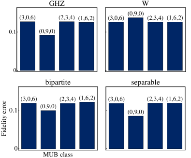
Figure 1: Fidelity errors of estimated GHZ and W states (upper panel) as well as bipartite and separable states (lower panel) for MUB tomography measurements. Notice that the bipartite-bases $(0,9,0)$ class performs best on GHZ, bipartite and separable states, but worst on W states. The differences are up to $30\%$.

In our simulations, genuinely tripartite GHZ and W entangled three-qubit states were randomly generated, as well as bipartite and separable ones, and subjected to MUB measurements. For each MUB class, the expected error of the inferred fidelity was estimated and averaged over $20,000$ randomly distributed states. The result is shown in Fig. 1. As we can appreciate, in average the $(0,9,0)$ scheme yields smaller fidelity errors for GHZ-like states (for bipartite and separable also) and larger errors for W states compared to other MUB sets. One also notices that the difference between GHZ, bipartite and separable is small, while W are still different.

To understand this result better, we have also investigated the noise in the measured data and calculated the correlations between the entropy of measurement probabilities and fidelity errors, restricting ourselves, for simplicity, to GHZ and W states. Figure 2 confirms strong correlations between those two magnitudes and shows that for GHZ states, $(0,9,0)$ tomograms are less noisy on average than $(3,0,6)$ tomograms. Again, the opposite is true for W states. There is not a simple connection between state entanglement and MUB classes, as one might naively anticipate. This demonstrates the key role played by error estimation along the lines presented here.

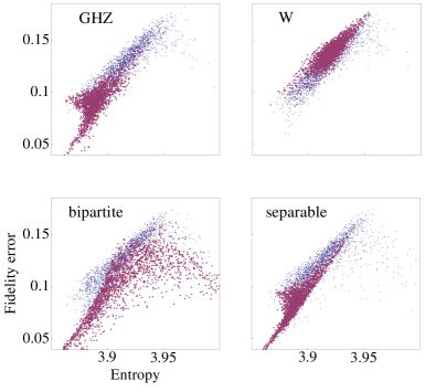
Figure 2: Correlations between the entropy of tomography outcomes and the corresponding fidelity errors for the same states as in Fig. 1. Large red and smalle blue dots are for $(0,9,0)$ and $(3,0,6)$ bases, respectively.

Finally, we consider a set of randomly chosen measurements $Z_{i}$, whose expectation values $\hat{z}_{i}=\mathop{\mathrm{Tr}}\nolimits(\hat{\rho}Z_{i})$ are inferred from the estimated state $\hat{\rho}$ and analyze the probability distribution $P[(\Delta z)^{2}]$ of the expected variances $\langle(\Delta z_{i})^{2}\rangle$. This distribution, being the real shadow $\langle z_{i}|\tilde{\mathrm{F}}^{-1}|z_{i}\rangle$ of the effective inverse Fisher matrix, tells us how the errors are distributed in the set of all possible measurements and hence describes in detail the performance of a given reconstruction scheme. In Fig. 3, the difference $\Delta P=P_{(0,9,0)}[(\Delta z)^{2}]-P_{(3,0,6)}[(\Delta z)^{2}]$ of the $(0,9,0)$ and $(3,0,6)$ shadows is approximated by histograms obtained from $500,000$ variances calculated for randomly generated measurements $|z_{i}\rangle$ and randomly choosen GHZ and W states for each MUB set. For GHZ states, the $(0,9,0)$ scheme yields very small errors and very large errors more often than the $(3,0,6)$ scheme. The opposite is true for W states. Such complementary behavior of different MUB sets makes it possible to optimize the tomography setup. For instance, quantities with low inherent noise are more precisely determined by the $(0,9,0)$ [$(3,0,6)$] set provided the true state is GHZ-like (W-like). The fidelity measurement discussed above is a salient example of that optimization.

We stress that this kind of analysis, where many repeated evaluations of the Fisher matrix must be performed, is chiefly suited to the proposed method, for the standard approach would become quickly unfeasible due to the scaling with the system dimension.

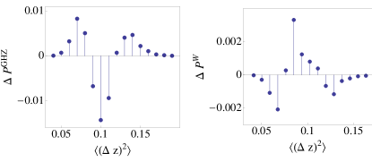
Figure 3: Differences of $(0,9,0)$ and $(3,0,6)$ histograms of variances for GHZ and W states. All histograms are normalized to unity. Positive $\Delta P$ for some $(\Delta z)^{2}$ means error of this size is more typical for $(0,9,0)$ scheme than for $(3,0,6)$ scheme and vice versa.

V Concluding remarks

To summarize, we have presented a complete Fisher-information-based toolbox for the proper assessment of any IC tomographic scheme. In this context, we have discussed the case of set of MUBs; although all of them are IC, their performance for some particular tasks turns out to be dependent on the entanglement distribution among the states of the set. We believe that the ideas and techniques developed here will be relevant in the experimental implementation and optimization of quantum protocols in higher-dimensional Hilbert spaces.

Explicit form of the set of MUBs for three qubits

For the sake of completeness, we briefly review the structure of the sets of MUBs for three qubits, following essentially the approach in Ref. Romero et al. (2005).

Because states belonging to the same basis are usually taken to be orthonormal, to study the property of “mutually unbiasedness” it is possible to use either mutually unbiased bases or the operators which have the basis states as eigenvectors. We thus need $d^{2}-1$ operators to obtain the whole set of states. In the case of power of prime dimension, this set can be constructed as $d+1$ classes of $d-1$ commuting operators.

In this way we get tables with nine rows of three mutually commuting (tensor products of) operators. We have suppressed the tensor multiplication sign in all the tables. By construction, the simultaneous eigenstates of the operators in each row give a complete basis, and each basis is mutually unbiased to each other. The number on the left enumerates the bases, while the number on the right denotes how many subsystems the bases can be factorized into.

As stated before, we label the different sets of MUBs by $(n_{1},n_{2},n_{3})$, where $n_{1}$ denotes the number of separable bases (every eigenvector of theses bases is a tensor product of singe-qubit states), $n_{2}$ the number of biseparable bases (one qubit is factorized and the other two are in a maximally entangled state) and $n_{3}$ the number of nonseparable bases. In this way, the allowed structures are $\{(2,3,4),(0,9,0),(1,6,2),(3,0,6)\}$ and the corresponding tables are given in the following.

Table 1: (2,3,4) MUB.

1	$\hat{\sigma}_{z}\hat{\openone}\hat{\openone}$	$\hat{\openone}\hat{\openone}\hat{\sigma}_{z}$	$\hat{\openone}\hat{\sigma}_{z}\hat{\openone}$	$\hat{\sigma}_{z}\hat{\openone}\hat{\sigma}_{z}$	$\hat{\openone}\hat{\sigma}_{z}\hat{\sigma}_{z}$	$\hat{\sigma}_{z}\hat{\sigma}_{z}\hat{\sigma}_{z}$	$\hat{\sigma}_{z}\hat{\sigma}_{z}\hat{\openone}$	3
2	$\hat{\sigma}_{x}\hat{\openone}\hat{\openone}$	$\hat{\openone}\hat{\sigma}_{x}\hat{\openone}$	$\hat{\openone}\hat{\openone}\hat{\sigma}_{x}$	$\hat{\sigma}_{x}\hat{\sigma}_{x}\hat{\openone}$	$\hat{\openone}\hat{\sigma}_{x}\hat{\sigma}_{x}$	$\hat{\sigma}_{x}\hat{\sigma}_{x}\hat{\sigma}_{x}$	$\hat{\sigma}_{x}\hat{\openone}\hat{\sigma}_{x}$	3
3	$\hat{\sigma}_{y}\hat{\openone}\hat{\openone}$	$\hat{\openone}\hat{\sigma}_{x}\hat{\sigma}_{z}$	$\hat{\openone}\hat{\sigma}_{z}\hat{\sigma}_{x}$	$\hat{\sigma}_{y}\hat{\sigma}_{x}\hat{\sigma}_{z}$	$\hat{\openone}\hat{\sigma}_{y}\hat{\sigma}_{y}$	$\hat{\sigma}_{y}\hat{\sigma}_{y}\hat{\sigma}_{y}$	$\hat{\sigma}_{y}\hat{\sigma}_{z}\hat{\sigma}_{x}$	2
4	$\hat{\sigma}_{x}\hat{\openone}\hat{\sigma}_{z}$	$\hat{\openone}\hat{\sigma}_{y}\hat{\openone}$	$\hat{\sigma}_{z}\hat{\openone}\hat{\sigma}_{y}$	$\hat{\sigma}_{x}\hat{\sigma}_{y}\hat{\sigma}_{z}$	$\hat{\sigma}_{z}\hat{\sigma}_{y}\hat{\sigma}_{y}$	$\hat{\sigma}_{y}\hat{\sigma}_{y}\hat{\sigma}_{x}$	$\hat{\sigma}_{y}\hat{\openone}\hat{\sigma}_{x}$	2
5	$\hat{\sigma}_{x}\hat{\sigma}_{z}\hat{\openone}$	$\hat{\sigma}_{z}\hat{\sigma}_{x}\hat{\sigma}_{z}$	$\hat{\openone}\hat{\sigma}_{z}\hat{\sigma}_{y}$	$\hat{\sigma}_{y}\hat{\sigma}_{y}\hat{\sigma}_{z}$	$\hat{\sigma}_{z}\hat{\sigma}_{y}\hat{\sigma}_{x}$	$\hat{\sigma}_{y}\hat{\sigma}_{x}\hat{\sigma}_{x}$	$\hat{\sigma}_{x}\hat{\openone}\hat{\sigma}_{y}$	1
6	$\hat{\sigma}_{y}\hat{\openone}\hat{\sigma}_{z}$	$\hat{\openone}\hat{\sigma}_{y}\hat{\sigma}_{z}$	$\hat{\sigma}_{z}\hat{\sigma}_{z}\hat{\sigma}_{y}$	$\hat{\sigma}_{y}\hat{\sigma}_{y}\hat{\openone}$	$\hat{\sigma}_{z}\hat{\sigma}_{x}\hat{\sigma}_{x}$	$\hat{\sigma}_{x}\hat{\sigma}_{x}\hat{\sigma}_{y}$	$\hat{\sigma}_{x}\hat{\sigma}_{z}\hat{\sigma}_{x}$	1
7	$\hat{\sigma}_{x}\hat{\sigma}_{z}\hat{\sigma}_{z}$	$\hat{\sigma}_{z}\hat{\sigma}_{y}\hat{\sigma}_{z}$	$\hat{\sigma}_{z}\hat{\sigma}_{z}\hat{\sigma}_{x}$	$\hat{\sigma}_{y}\hat{\sigma}_{x}\hat{\openone}$	$\hat{\openone}\hat{\sigma}_{x}\hat{\sigma}_{y}$	$\hat{\sigma}_{x}\hat{\sigma}_{y}\hat{\sigma}_{x}$	$\hat{\sigma}_{y}\hat{\openone}\hat{\sigma}_{y}$	1
8	$\hat{\sigma}_{y}\hat{\sigma}_{z}\hat{\sigma}_{z}$	$\hat{\sigma}_{z}\hat{\sigma}_{y}\hat{\openone}$	$\hat{\sigma}_{z}\hat{\openone}\hat{\sigma}_{x}$	$\hat{\sigma}_{x}\hat{\sigma}_{x}\hat{\sigma}_{z}$	$\hat{\openone}\hat{\sigma}_{y}\hat{\sigma}_{x}$	$\hat{\sigma}_{y}\hat{\sigma}_{x}\hat{\sigma}_{y}$	$\hat{\sigma}_{x}\hat{\sigma}_{z}\hat{\sigma}_{y}$	1
9	$\hat{\sigma}_{y}\hat{\sigma}_{z}\hat{\openone}$	$\hat{\sigma}_{z}\hat{\sigma}_{x}\hat{\openone}$	$\hat{\openone}\hat{\openone}\hat{\sigma}_{y}$	$\hat{\sigma}_{x}\hat{\sigma}_{y}\hat{\openone}$	$\hat{\sigma}_{z}\hat{\sigma}_{x}\hat{\sigma}_{y}$	$\hat{\sigma}_{x}\hat{\sigma}_{y}\hat{\sigma}_{y}$	$\hat{\sigma}_{y}\hat{\sigma}_{z}\hat{\sigma}_{y}$	2

Table 2: (0,9,0) MUB.

1	$\hat{\sigma}_{x}\hat{\openone}\hat{\openone}$	$\hat{\openone}\hat{\sigma}_{z}\hat{\sigma}_{y}$	$\hat{\openone}\hat{\sigma}_{y}\hat{\sigma}_{z}$	$\hat{\sigma}_{x}\hat{\sigma}_{z}\hat{\sigma}_{y}$	$\hat{\openone}\hat{\sigma}_{x}\hat{\sigma}_{x}$	$\hat{\sigma}_{x}\hat{\sigma}_{x}\hat{\sigma}_{x}$	$\hat{\sigma}_{x}\hat{\sigma}_{y}\hat{\sigma}_{z}$	2
2	$\hat{\sigma}_{y}\hat{\openone}\hat{\openone}$	$\hat{\openone}\hat{\sigma}_{x}\hat{\sigma}_{z}$	$\hat{\openone}\hat{\sigma}_{z}\hat{\sigma}_{x}$	$\hat{\sigma}_{y}\hat{\sigma}_{x}\hat{\sigma}_{z}$	$\hat{\openone}\hat{\sigma}_{y}\hat{\sigma}_{y}$	$\hat{\sigma}_{y}\hat{\sigma}_{y}\hat{\sigma}_{y}$	$\hat{\sigma}_{y}\hat{\sigma}_{z}\hat{\sigma}_{x}$	2
3	$\hat{\sigma}_{z}\hat{\openone}\hat{\openone}$	$\hat{\openone}\hat{\sigma}_{y}\hat{\sigma}_{x}$	$\hat{\openone}\hat{\sigma}_{x}\hat{\sigma}_{y}$	$\hat{\sigma}_{z}\hat{\sigma}_{y}\hat{\sigma}_{x}$	$\hat{\openone}\hat{\sigma}_{z}\hat{\sigma}_{z}$	$\hat{\sigma}_{z}\hat{\sigma}_{z}\hat{\sigma}_{z}$	$\hat{\sigma}_{z}\hat{\sigma}_{x}\hat{\sigma}_{y}$	2
4	$\hat{\sigma}_{y}\hat{\sigma}_{z}\hat{\sigma}_{y}$	$\hat{\openone}\hat{\sigma}_{z}\hat{\openone}$	$\hat{\sigma}_{x}\hat{\openone}\hat{\sigma}_{z}$	$\hat{\sigma}_{y}\hat{\openone}\hat{\sigma}_{y}$	$\hat{\sigma}_{x}\hat{\sigma}_{z}\hat{\sigma}_{z}$	$\hat{\sigma}_{z}\hat{\openone}\hat{\sigma}_{x}$	$\hat{\sigma}_{z}\hat{\sigma}_{z}\hat{\sigma}_{x}$	2
5	$\hat{\sigma}_{y}\hat{\sigma}_{y}\hat{\sigma}_{z}$	$\hat{\sigma}_{x}\hat{\sigma}_{y}\hat{\sigma}_{x}$	$\hat{\openone}\hat{\sigma}_{y}\hat{\openone}$	$\hat{\sigma}_{z}\hat{\openone}\hat{\sigma}_{y}$	$\hat{\sigma}_{x}\hat{\openone}\hat{\sigma}_{x}$	$\hat{\sigma}_{z}\hat{\sigma}_{y}\hat{\sigma}_{y}$	$\hat{\sigma}_{y}\hat{\openone}\hat{\sigma}_{z}$	2
6	$\hat{\sigma}_{z}\hat{\sigma}_{z}\hat{\sigma}_{y}$	$\hat{\openone}\hat{\openone}\hat{\sigma}_{y}$	$\hat{\sigma}_{x}\hat{\sigma}_{y}\hat{\openone}$	$\hat{\sigma}_{z}\hat{\sigma}_{z}\hat{\openone}$	$\hat{\sigma}_{x}\hat{\sigma}_{y}\hat{\sigma}_{y}$	$\hat{\sigma}_{y}\hat{\sigma}_{x}\hat{\openone}$	$\hat{\sigma}_{y}\hat{\sigma}_{x}\hat{\sigma}_{y}$	2
7	$\hat{\sigma}_{y}\hat{\sigma}_{x}\hat{\sigma}_{x}$	$\hat{\sigma}_{x}\hat{\openone}\hat{\sigma}_{y}$	$\hat{\sigma}_{x}\hat{\sigma}_{x}\hat{\sigma}_{y}$	$\hat{\sigma}_{z}\hat{\sigma}_{x}\hat{\sigma}_{z}$	$\hat{\openone}\hat{\sigma}_{x}\hat{\openone}$	$\hat{\sigma}_{y}\hat{\openone}\hat{\sigma}_{x}$	$\hat{\sigma}_{z}\hat{\openone}\hat{\sigma}_{z}$	2
8	$\hat{\sigma}_{z}\hat{\sigma}_{x}\hat{\sigma}_{x}$	$\hat{\sigma}_{x}\hat{\sigma}_{z}\hat{\openone}$	$\hat{\sigma}_{x}\hat{\sigma}_{z}\hat{\sigma}_{x}$	$\hat{\sigma}_{y}\hat{\sigma}_{y}\hat{\sigma}_{x}$	$\hat{\openone}\hat{\openone}\hat{\sigma}_{x}$	$\hat{\sigma}_{z}\hat{\sigma}_{x}\hat{\openone}$	$\hat{\sigma}_{y}\hat{\sigma}_{y}\hat{\openone}$	2
9	$\hat{\sigma}_{z}\hat{\sigma}_{y}\hat{\sigma}_{z}$	$\hat{\sigma}_{x}\hat{\sigma}_{x}\hat{\sigma}_{z}$	$\hat{\openone}\hat{\openone}\hat{\sigma}_{z}$	$\hat{\sigma}_{y}\hat{\sigma}_{z}\hat{\openone}$	$\hat{\sigma}_{x}\hat{\sigma}_{x}\hat{\openone}$	$\hat{\sigma}_{y}\hat{\sigma}_{z}\hat{\sigma}_{z}$	$\hat{\sigma}_{z}\hat{\sigma}_{y}\hat{\openone}$	2

Table 3: (1,6,2) MUB.

1	$\hat{\sigma}_{x}\hat{\sigma}_{z}\hat{\openone}$	$\hat{\openone}\hat{\openone}\hat{\sigma}_{y}$	$\hat{\sigma}_{z}\hat{\sigma}_{y}\hat{\openone}$	$\hat{\sigma}_{x}\hat{\sigma}_{z}\hat{\sigma}_{y}$	$\hat{\sigma}_{z}\hat{\sigma}_{y}\hat{\sigma}_{y}$	$\hat{\sigma}_{y}\hat{\sigma}_{x}\hat{\sigma}_{y}$	$\hat{\sigma}_{y}\hat{\sigma}_{x}\hat{\openone}$	2
2	$\hat{\sigma}_{y}\hat{\sigma}_{z}\hat{\openone}$	$\hat{\sigma}_{z}\hat{\sigma}_{x}\hat{\openone}$	$\hat{\openone}\hat{\openone}\hat{\sigma}_{x}$	$\hat{\sigma}_{x}\hat{\sigma}_{y}\hat{\openone}$	$\hat{\sigma}_{z}\hat{\sigma}_{x}\hat{\sigma}_{x}$	$\hat{\sigma}_{x}\hat{\sigma}_{y}\hat{\sigma}_{x}$	$\hat{\sigma}_{y}\hat{\sigma}_{z}\hat{\sigma}_{x}$	2
3	$\hat{\sigma}_{z}\hat{\openone}\hat{\openone}$	$\hat{\sigma}_{z}\hat{\sigma}_{x}\hat{\sigma}_{y}$	$\hat{\sigma}_{z}\hat{\sigma}_{y}\hat{\sigma}_{x}$	$\hat{\openone}\hat{\sigma}_{x}\hat{\sigma}_{y}$	$\hat{\openone}\hat{\sigma}_{z}\hat{\sigma}_{z}$	$\hat{\sigma}_{z}\hat{\sigma}_{z}\hat{\sigma}_{z}$	$\hat{\openone}\hat{\sigma}_{y}\hat{\sigma}_{x}$	2
4	$\hat{\sigma}_{y}\hat{\sigma}_{z}\hat{\sigma}_{y}$	$\hat{\openone}\hat{\sigma}_{z}\hat{\openone}$	$\hat{\sigma}_{x}\hat{\sigma}_{z}\hat{\sigma}_{z}$	$\hat{\sigma}_{y}\hat{\openone}\hat{\sigma}_{y}$	$\hat{\sigma}_{x}\hat{\openone}\hat{\sigma}_{z}$	$\hat{\sigma}_{z}\hat{\sigma}_{z}\hat{\sigma}_{x}$	$\hat{\sigma}_{z}\hat{\openone}\hat{\sigma}_{x}$	2
5	$\hat{\sigma}_{x}\hat{\sigma}_{x}\hat{\openone}$	$\hat{\sigma}_{y}\hat{\sigma}_{y}\hat{\sigma}_{y}$	$\hat{\sigma}_{z}\hat{\sigma}_{y}\hat{\sigma}_{z}$	$\hat{\sigma}_{z}\hat{\sigma}_{z}\hat{\sigma}_{y}$	$\hat{\sigma}_{x}\hat{\openone}\hat{\sigma}_{x}$	$\hat{\openone}\hat{\sigma}_{x}\hat{\sigma}_{x}$	$\hat{\sigma}_{y}\hat{\sigma}_{z}\hat{\sigma}_{z}$	1
6	$\hat{\sigma}_{z}\hat{\openone}\hat{\sigma}_{y}$	$\hat{\openone}\hat{\sigma}_{z}\hat{\sigma}_{y}$	$\hat{\sigma}_{y}\hat{\sigma}_{x}\hat{\sigma}_{z}$	$\hat{\sigma}_{z}\hat{\sigma}_{z}\hat{\openone}$	$\hat{\sigma}_{y}\hat{\sigma}_{y}\hat{\sigma}_{x}$	$\hat{\sigma}_{x}\hat{\sigma}_{y}\hat{\sigma}_{z}$	$\hat{\sigma}_{x}\hat{\sigma}_{x}\hat{\sigma}_{x}$	1
7	$\hat{\sigma}_{x}\hat{\sigma}_{x}\hat{\sigma}_{y}$	$\hat{\sigma}_{x}\hat{\openone}\hat{\sigma}_{y}$	$\hat{\sigma}_{y}\hat{\sigma}_{x}\hat{\sigma}_{x}$	$\hat{\openone}\hat{\sigma}_{x}\hat{\openone}$	$\hat{\sigma}_{z}\hat{\sigma}_{x}\hat{\sigma}_{z}$	$\hat{\sigma}_{y}\hat{\openone}\hat{\sigma}_{x}$	$\hat{\sigma}_{z}\hat{\openone}\hat{\sigma}_{z}$	2
8	$\hat{\openone}\hat{\sigma}_{y}\hat{\sigma}_{y}$	$\hat{\sigma}_{x}\hat{\openone}\hat{\openone}$	$\hat{\sigma}_{x}\hat{\sigma}_{z}\hat{\sigma}_{x}$	$\hat{\sigma}_{x}\hat{\sigma}_{y}\hat{\sigma}_{y}$	$\hat{\openone}\hat{\sigma}_{z}\hat{\sigma}_{x}$	$\hat{\openone}\hat{\sigma}_{x}\hat{\sigma}_{z}$	$\hat{\sigma}_{x}\hat{\sigma}_{x}\hat{\sigma}_{z}$	2
9	$\hat{\openone}\hat{\sigma}_{y}\hat{\openone}$	$\hat{\sigma}_{y}\hat{\sigma}_{y}\hat{\openone}$	$\hat{\openone}\hat{\openone}\hat{\sigma}_{z}$	$\hat{\sigma}_{y}\hat{\openone}\hat{\openone}$	$\hat{\sigma}_{y}\hat{\sigma}_{y}\hat{\sigma}_{z}$	$\hat{\sigma}_{y}\hat{\openone}\hat{\sigma}_{z}$	$\hat{\openone}\hat{\sigma}_{y}\hat{\sigma}_{z}$	3

Table 4: (3,0,6) MUB.

1	$\hat{\sigma}_{x}\hat{\sigma}_{y}\hat{\sigma}_{z}$	$\hat{\openone}\hat{\sigma}_{z}\hat{\sigma}_{x}$	$\hat{\sigma}_{y}\hat{\sigma}_{z}\hat{\openone}$	$\hat{\sigma}_{x}\hat{\sigma}_{x}\hat{\sigma}_{y}$	$\hat{\sigma}_{y}\hat{\openone}\hat{\sigma}_{x}$	$\hat{\sigma}_{z}\hat{\sigma}_{y}\hat{\sigma}_{y}$	$\hat{\sigma}_{z}\hat{\sigma}_{x}\hat{\sigma}_{z}$	1
2	$\hat{\sigma}_{z}\hat{\sigma}_{y}\hat{\sigma}_{z}$	$\hat{\sigma}_{y}\hat{\sigma}_{x}\hat{\sigma}_{z}$	$\hat{\openone}\hat{\sigma}_{z}\hat{\sigma}_{y}$	$\hat{\sigma}_{x}\hat{\sigma}_{z}\hat{\openone}$	$\hat{\sigma}_{y}\hat{\sigma}_{y}\hat{\sigma}_{x}$	$\hat{\sigma}_{x}\hat{\openone}\hat{\sigma}_{y}$	$\hat{\sigma}_{z}\hat{\sigma}_{x}\hat{\sigma}_{x}$	1
3	$\hat{\sigma}_{y}\hat{\openone}\hat{\openone}$	$\hat{\sigma}_{y}\hat{\sigma}_{y}\hat{\sigma}_{y}$	$\hat{\sigma}_{y}\hat{\openone}\hat{\sigma}_{y}$	$\hat{\openone}\hat{\sigma}_{y}\hat{\sigma}_{y}$	$\hat{\openone}\hat{\sigma}_{y}\hat{\openone}$	$\hat{\sigma}_{y}\hat{\sigma}_{y}\hat{\openone}$	$\hat{\openone}\hat{\openone}\hat{\sigma}_{y}$	3
4	$\hat{\sigma}_{z}\hat{\sigma}_{x}\hat{\sigma}_{y}$	$\hat{\openone}\hat{\sigma}_{y}\hat{\sigma}_{z}$	$\hat{\sigma}_{x}\hat{\sigma}_{y}\hat{\openone}$	$\hat{\sigma}_{z}\hat{\sigma}_{z}\hat{\sigma}_{x}$	$\hat{\sigma}_{x}\hat{\openone}\hat{\sigma}_{z}$	$\hat{\sigma}_{y}\hat{\sigma}_{x}\hat{\sigma}_{x}$	$\hat{\sigma}_{y}\hat{\sigma}_{z}\hat{\sigma}_{y}$	1
5	$\hat{\sigma}_{x}\hat{\sigma}_{x}\hat{\sigma}_{z}$	$\hat{\sigma}_{z}\hat{\openone}\hat{\sigma}_{x}$	$\hat{\sigma}_{y}\hat{\sigma}_{z}\hat{\sigma}_{z}$	$\hat{\sigma}_{y}\hat{\sigma}_{x}\hat{\sigma}_{y}$	$\hat{\sigma}_{x}\hat{\sigma}_{z}\hat{\sigma}_{y}$	$\hat{\openone}\hat{\sigma}_{y}\hat{\sigma}_{x}$	$\hat{\sigma}_{z}\hat{\sigma}_{y}\hat{\openone}$	1
6	$\hat{\sigma}_{y}\hat{\sigma}_{z}\hat{\sigma}_{x}$	$\hat{\openone}\hat{\sigma}_{x}\hat{\sigma}_{y}$	$\hat{\sigma}_{z}\hat{\sigma}_{x}\hat{\openone}$	$\hat{\sigma}_{y}\hat{\sigma}_{y}\hat{\sigma}_{z}$	$\hat{\sigma}_{z}\hat{\openone}\hat{\sigma}_{y}$	$\hat{\sigma}_{x}\hat{\sigma}_{z}\hat{\sigma}_{z}$	$\hat{\sigma}_{x}\hat{\sigma}_{y}\hat{\sigma}_{x}$	1
7	$\hat{\sigma}_{x}\hat{\sigma}_{y}\hat{\sigma}_{y}$	$\hat{\sigma}_{x}\hat{\sigma}_{z}\hat{\sigma}_{x}$	$\hat{\sigma}_{z}\hat{\sigma}_{y}\hat{\sigma}_{x}$	$\hat{\openone}\hat{\sigma}_{x}\hat{\sigma}_{z}$	$\hat{\sigma}_{y}\hat{\sigma}_{x}\hat{\openone}$	$\hat{\sigma}_{z}\hat{\sigma}_{z}\hat{\sigma}_{y}$	$\hat{\sigma}_{y}\hat{\openone}\hat{\sigma}_{z}$	1
8	$\hat{\openone}\hat{\openone}\hat{\sigma}_{x}$	$\hat{\sigma}_{x}\hat{\openone}\hat{\openone}$	$\hat{\sigma}_{x}\hat{\sigma}_{x}\hat{\sigma}_{x}$	$\hat{\sigma}_{x}\hat{\openone}\hat{\sigma}_{x}$	$\hat{\openone}\hat{\sigma}_{x}\hat{\sigma}_{x}$	$\hat{\openone}\hat{\sigma}_{x}\hat{\openone}$	$\hat{\sigma}_{x}\hat{\sigma}_{x}\hat{\openone}$	3
9	$\hat{\openone}\hat{\sigma}_{z}\hat{\openone}$	$\hat{\sigma}_{z}\hat{\sigma}_{z}\hat{\openone}$	$\hat{\openone}\hat{\openone}\hat{\sigma}_{z}$	$\hat{\sigma}_{z}\hat{\openone}\hat{\openone}$	$\hat{\sigma}_{z}\hat{\sigma}_{z}\hat{\sigma}_{z}$	$\hat{\sigma}_{z}\hat{\openone}\hat{\sigma}_{z}$	$\hat{\openone}\hat{\sigma}_{z}\hat{\sigma}_{z}$	3

References

• Born (1926) M. Born, Z. Phys. 37, 863 (1926).
• Bohr (1935) N. Bohr, Phys. Rev. 48, 696 (1935).
• Helstrom (1976) C. W. Helstrom, Quantum Detection and Estimation Theory (Academic, New York, 1976).
• Holevo (2003) A. S. Holevo, Probabilistic and Statistical Aspects of Quantum Theory, 2nd ed. (North Holland, Amsterdam, 2003).
• Paris and Řeháček (2004) M. G. A. Paris and J. Řeháček, eds., Quantum State Estimation, Lect. Not. Phys., Vol. 649 (Springer, Berlin, 2004).
• Schwinger (1960a) J. Schwinger, Proc. Natl. Acad. Sci. USA 46, 570 (1960a).
• Schwinger (1960b) J. Schwinger, Proc. Natl. Acad. Sci. USA 46, 883 (1960b).
• Schwinger (1960c) J. Schwinger, Proc. Natl. Acad. Sci. USA 46, 1401 (1960c).
• Durt et al. (2010) T. Durt, B.-G. Englert, I. Bengtsson,  and K. Zyczkowski, Int. J. Quantum Inf. 8, 535 (2010).
• Wootters and Fields (1989) W. K. Wootters and B. D. Fields, Ann. Phys. 191, 363 (1989).
• Ivanovic (1981) I. D. Ivanovic, J. Phys. A 14, 3241 (1981).
• Lawrence et al. (2002) J. Lawrence, Č. Brukner,  and A. Zeilinger, Phys. Rev. A 65, 032320 (2002).
• Romero et al. (2005) J. L. Romero, G. Björk, A. B. Klimov,  and L. L. Sánchez-Soto, Phys. Rev. A 72, 062310 (2005).
• Lawrence (2011) J. Lawrence, Phys. Rev. A 84, 022338 (2011).
• Wieśniak et al. (2011) M. Wieśniak, T. Paterek,  and A. Zeilinger, New J. Phys. 13, 053047 (2011).
• Hioe and Eberly (1981) F. T. Hioe and J. H. Eberly, Phys. Rev. Lett. 47, 838 (1981).
• Kimura (2003) G. Kimura, Phys. Lett. A 314, 339 (2003).
• Cramér (1946) H. Cramér, Mathematical Methods of Statistics (Princeton University, Princeton, 1946).
• Rao (1973) C. R. Rao, Linear Statistical Inference and Its Applications (Wiley, New York, 1973).
• Fisher (1922) R. A. Fisher, Phil. Trans. R. Soc. A 222, 309 (1922).
• Strassen (1969) V. Strassen, Numer. Math. 13, 354 (1969).
• Prugovečki (1977) E. Prugovečki, Int. J. Theor. Phys. 16, 321 (1977).
• Busch and Lahti (1989) P. Busch and P. J. Lahti, Found. Phys. 19, 633 (1989).
• Ariano et al. (2004) G. M. D. Ariano, P. Perinotti,  and M. F. Sacchi, J. Opt. B 6, S487 (2004).
• Sych et al. (2012) D. Sych, J. Řeháček, Z. Hradil, G. Leuchs,  and L. L. Sánchez-Soto, Phys. Rev. A 86, 052123 (2012).
• Zhu and Englert (2011) H. Zhu and B.-G. Englert, Phys. Rev. A 84, 022327 (2011).
• Dunkl et al. (2011) C. F. Dunkl, P. Gawron, J. A. Holbrook, J. A. Miszczak, Z. Puchała,  and K. Życzkowski, J. Phys. A 44, 335301 (2011).