A Component Lasso

Abstract

We propose a new sparse regression method called the component lasso, based on a simple idea. The method uses the connected-components structure of the sample covariance matrix to split the problem into smaller ones. It then applies the lasso to each subproblem separately, obtaining a coefficient vector for each one. Finally, it uses non-negative least squares to recombine the different vectors into a single solution. This step is useful in selecting and reweighting components that are correlated with the response. Simulated and real data examples show that the component lasso can outperform standard regression methods such as the lasso and elastic net, achieving a lower mean squared error as well as better support recovery. The modular structure also lends itself naturally to parallel computation.

Keywords. Lasso, elastic net, graphical lasso, sparsity, connected components, $\ell_{1}$-minimization, non-negative least squares, grouping effect.

1 Introduction

Suppose that we have a response vector $y\in\mathds{R}^{n}$, a matrix $X\in\mathds{R}^{n\times p}$ of predictor variables and the usual linear regression setup:

$$y=X\beta^{*}+\sigma\epsilon,$$ (1)

where $\beta^{*}\in\mathds{R}^{p}$ are unknown coefficients to be estimated, $\sigma^{2}>0$ is the noise variance, and the components of the noise vector $\epsilon\in\mathds{R}^{n}$ are i.i.d. with $\mathbb{E}[\epsilon_{i}]=0$ and $\mathrm{Var}(\epsilon_{i})=1$. We assume that $y$ has been centered, and the columns of $X$ are centered and scaled, so that we can omit an intercept in the model. The lasso estimator [lasso, bp], is defined as

$$\hat{\beta}=\mathop{\mathrm{argmin}}_{\beta\in\mathds{R}^{p}}\,\frac{1}{2}\|y-X\beta\|_{2}^{2}+\lambda\|\beta\|_{1},$$ (2)

where $\lambda\geq 0$ is a tuning parameter, controlling the degree of sparsity in the estimate $\hat{\beta}$.

Variable selection is important in many modern applications, for which the lasso has proven to be successful. However, this method has known limitations in certain settings: there is a solution with at most $n$ non-zero coefficients when $p>n$, and if a group of relevant variables is highly correlated, it tends to include only one in the model. These conditions occur frequently in real applications, such as genomics, where we often have a large number of predictors that can be divided into highly correlated groups. It is therefore of practical interest to overcome these limitations.

The elastic net  [enet] can sometimes improve the performance of the lasso. The elastic net penalty is the weighted sum of the $\ell_{2}$ and $\ell_{1}$ norms of the coefficient vector to be estimated: $P_{\alpha}(\beta)=\frac{(1-\alpha)}{2}||\beta||_{2}^{2}+\alpha||\beta||_{1}$. It is equivalent to the ridge regression penalty when $\alpha=0$, and to the lasso penalty when $\alpha=1$. The elastic net solves the following problem:

$$\hat{\beta}=\mathop{\mathrm{argmin}}_{\beta\in\mathds{R}^{p}}\,\frac{1}{2}\|y-X\beta\|_{2}^{2}+\lambda P_{\alpha}(\beta).$$ (3)

The elastic net penalty is strictly convex, by strict convexity of the $\ell_{2}$ norm. Using this fact, the authors provide an upper bound on the distance between coefficients that correspond to highly correlated predictors. This guarantees the grouping effect of the elastic net. Moreover, the elastic net solution can have more than $n$ non-zero coefficients, even when $p>n$, since it is equivalent to solving the lasso on an augmented dataset.

It is easy to see that the elastic net regularizes the feature covariance matrix from $X^{T}X$ to a form $X^{T}X+\frac{1-\alpha}{2}\cdot\lambda I_{p}$ where $I_{p}$ is the $p\times p$ identity matrix. By inflating the diagonal it reduces the effective size of the off-diagonal correlations. If the feature covariance matrix is block diagonal, its connected components correspond to groups of predictors that are correlated with each other but not with predictors in other groups. Here, we introduce a method adapted to situations where the sample covariance matrix is approximately block diagonal. Our proposed method, the component lasso, applies a more severe form of decorrelation than the elastic net to exploit this structure.

Consider the inverse of the covariance matrix of the predictors. Zeros in this matrix correspond to conditionally independent variables. Recent work has focused on estimating a sparse version of the inverse covariance by optimizing the $\ell_{1}$ penalized log-likelihood. The so-called “graphical lasso” algorithm solves the problem by cycling through the variables and fitting a modified lasso regression to each one. In their “scout” procedure, WT2009 used the graphical lasso in a penalized regression framework to estimate the inverse covariance of $X$. Then they applied a modified form of the lasso to estimate the regression parameters.

More recently, a connection between the graphical lasso and connected components has been established by WFS2011 and MH2012. Specifically, the connected components in the estimated inverse covariance matrix correspond exactly to those obtained from single-linkage clustering of the correlation matrix. Clustering the correlated variables before estimating the parameters has been suggested by GE2007 and BUH2007.

In this paper, we propose a new simple idea to make use of the connected components in penalized regression. The component lasso works by (a) finding the connected components of the estimated covariance matrix, (b) solving separate lasso problems for each component, and then (c) combining the componentwise predictions into one final prediction. We show that this approach can improve the accuracy, and interpretability of the lasso and elastic net methods. The method is summarized in Figure 1.

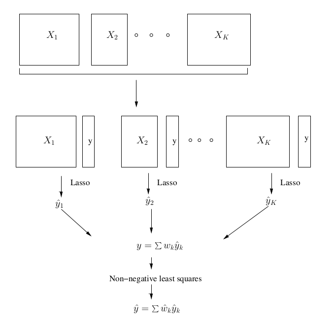
Figure 1: The component lasso steps: The predictors are split according to the estimated connected components of the sample covariance matrix. The lasso is applied to each subset of predictors to separately estimate the coefficients and to predict the response. Finally, the different coefficient vectors are combined using a non-negative least squares fit of $y$ on the $K$ predictions from each component.

The following example motivates the remainder of the paper. Consider eight predictors, and let the corresponding covariance matrix be block diagonal with two blocks. Suppose that the predictors corresponding to the first block, or equivalently component, are all signal variables. The second component only contains noise variables. Figure 2 shows the coefficient paths for the naive and non naive elastic net, and the component lasso before and after the non-negative least squares (NNLS) recombination step when the sample covariance is split into two blocks. The paths are plotted for all values of the tuning parameter $\lambda$.

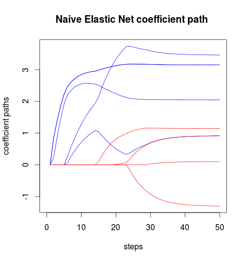
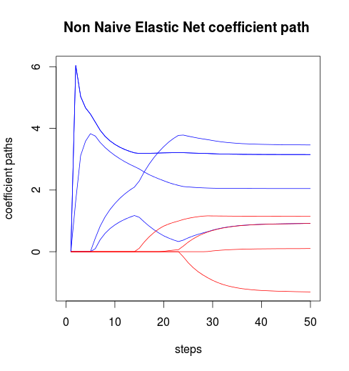
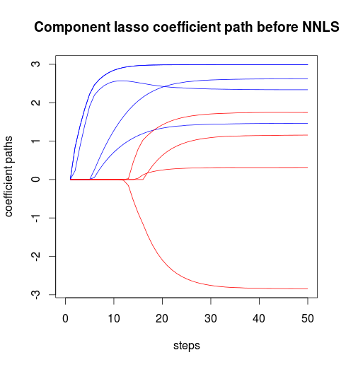
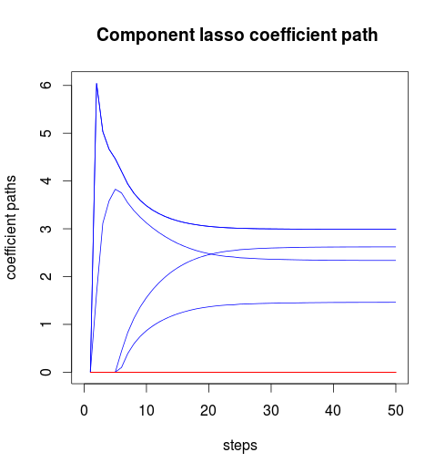
Figure 2: Coefficient paths for : the naive elastic net (top left), the non naive elastic net (top right), the component lasso before non-negative least squares (bottom left), and the component lasso (bottom right). The signal variables are shown in blue, while the non-signal variables are in red.

The example shows the role that NNLS plays in selecting the relevant component which contains the signal variables (in blue) and reducing the coefficients of the noise variables (in red) in the second component to zero. This illustrates the possible improvements that can be achieved by finding the block-diagonal structure of the sample covariance matrix, as compared to standard methods.

The remainder of the paper is organized as follows. We explain our algorithm in Section 2. Section 3 includes simulated and real data results. Section 4 focuses on the computational complexity of the component lasso, and presents ideas for making it more efficient. We conclude the paper with a short discussion in Section 5, including possible extensions to generalized linear models.

2 The Component Lasso

2.1 The main idea

The lasso minimizes the $\ell_{1}$ penalized criterion (2) whose corresponding subgradient equation is

$$X^{T}X\beta-X^{T}y+\lambda\cdot\text{sign}(\beta)=0,$$ (4)

where $\text{sign}(\beta)$ is a vector with components $s_{j}=\text{sign}(\beta_{j})$ if $\beta_{j}\neq 0$ and $s_{j}\in[-1,1]$ if $\beta_{j}=0$.

The solution to the lasso can be written as

$$\hat{\beta}=(X^{T}X)^{-}(X^{T}y-\lambda\cdot\text{sign}(\hat{\beta}))$$ (5)

where $(X^{T}X)^{-}$ represents a generalized inverse of $X^{T}X$.

Let $\Sigma=\text{cov}(X)$. We propose replacing $(X^{T}X)^{-}$ by a block diagonal estimate $n^{-1}\hat{\Theta}\approx n^{-1}\Sigma^{-1}$, the blocks of $\hat{\Theta}$ being the (estimated) connected components. Finding $K$ connected components splits the subgradient equation into $K$ separate equations:

$$X^{T}_{k}X_{k}\beta_{k}-X_{k}^{T}y+\lambda\cdot\text{sign}(\beta_{k})=0$$ (6)

for $k=1,2,\dots K$, where $X_{k}$ is a subset of $X$ containing the observations of the predictors in the $k$th component, and $\beta_{k}$ contains the corresponding coefficients.

Each subproblem can be solved individually using a standard lasso or elastic net algorithm. The resultant coefficients $\beta_{k}$ are then combined into a solution to the original problem. The use of the block-diagonal covariance matrix creates a substantial bias in the coefficient estimates, so the combination step is quite important. We scale the componentwise solution vectors $\hat{\beta}_{1},\hat{\beta}_{2},\ldots\hat{\beta}_{K}$ using a non-negative least squares refitting of $y$ on $\{\hat{y}_{k}=X_{k}\hat{\beta}_{k}\},k=1,\dots,K$. The non-negativity constraint seems natural since each componentwise predictor should have positive correlation with the outcome.

The component lasso objective function, corresponding to a block diagonal estimate of the sample covariance with connected components $C_{1},\dots,C_{K}$ is:

$$J(\beta,c)=\sum_{k=1}^{K}\sum_{i=1}^{n}\left[\frac{1}{2}\left(y_{i}-c_{k}\sum_{j\in C_{k}}X_{ij}\beta_{j}\right)^{2}+\lambda\left(\sum_{j\in C_{k}}\alpha|\beta_{j}|+\frac{(1-\alpha)}{2}||\beta_{j}||_{2}^{2}\right)\;\right]$$ (7)

subject to $c_{k}\geq 0\;\forall k$. Our algorithm (detailed below) sets $c_{k}=1\;\forall k$, optimizes over $\beta$, and then optimizes over $c$.

Consider an extreme case where the sample covariance matrix happens to be block diagonal with $K$ connected components. This occurs when predictors in different correlated groups are orthogonal to each other. The subgradient equation of the lasso splits naturally into separate systems of equations as in equation (6) for the component lasso. The lasso coefficients will be identical to the component lasso coefficients before the NNLS step, which reweights the predictors corresponding to each component.

This can be easily extended to the elastic net. Let $\lambda^{\prime}=\frac{\lambda(1-\alpha)}{2}$ be the tuning parameter corresponding to the $\ell_{2}$ penalty. The naive elastic net problem can be written as a lasso problem on an augmented data set $(y^{*},X^{*})$, where $y^{*}=(y,0)$ is now an $n+p$ vector and

$$X^{*}=(1+\lambda^{\prime})^{-1/2}\left[\begin{array}[]{c}X\\ \sqrt{\lambda^{\prime}}I\end{array}\right].$$

The sample covariance matrix corresponding to the augmented observations $X^{*}$

$$(1+\lambda^{\prime})^{-1}(X^{T}X+\lambda^{\prime}I)$$

is clearly block diagonal when the predictors in different components are orthogonal.

Therefore, the subgradient equation of the elastic net splits as well, and the elastic net coefficients will be identical to those of the component lasso before the NNLS step. In this case, the model chosen by the component lasso will involve splitting the predictors into components if the NNLS reweighting is useful in minimizing the validation MSE.

2.2 Details of connected component estimation via the graphical lasso

Given an observed covariance $S={X^{T}X/n}$ with $X\sim\mathcal{N}(0,\Sigma)$, the graphical lasso estimates $\Theta=\Sigma^{-1}$ by maximizing the penalized log-likelihood

$$\ell(\Theta)=\log{\rm det}\Theta-{\rm tr}(S\Theta)-\tau||\Theta||_{1}$$ (8)

over all non-negative definite matrices $\Theta$ . The KKT conditions for this problem are

$$\Theta^{-1}=S-\tau\Gamma(\Theta)=0$$ (9)

where $\Gamma(\Theta)$ is a matrix of componentwise subgradients $\text{sign}(\Theta_{ij})$. If $C_{1},C_{2}\ldots C_{K}$ are a partition of $1,2,\ldots p$, then WFS2011 and MH2012 show that the corresponding arrangement of $\hat{\Theta}(\tau)$ is block diagonal if and only if $S_{ii^{\prime}}\leq\tau$ for all $i\in C_{k},i^{\prime}\in C_{k^{\prime}},k\neq k^{\prime}$. This means that soft-thresholding of $S$ at level $\tau$ into its connected components yields the connected components of $\hat{\Theta}(\tau)$.

Furthermore, there is an interesting connection to hierarchical clustering. Specifically the connected components correspond to the subtrees from when we apply single linkage agglomerative clustering to $S$ and then cut the dendrogram at level $\tau$ [TWS2013]. Single linkage clustering is sometimes not very attractive in practice, since it can produce long and stringy clusters and hence components of very unequal size. However, these same authors show that under regularity conditions on $S$, application of average or complete linkage agglomerative clustering also consistently estimates the connected components. Hence we are free to use average, single or complete linkage clustering; we use average linkage in the examples of this paper.

2.3 Summary of the component lasso algorithm

1. Apply average, single or complete linkage clustering to $S=X^{T}X/n$ and cut the dendrogram at level $\tau$ to produce components $C_{1},C_{2},\ldots C_{K}$.

2. For each component $k=1,2,\ldots K$ and fixed elastic net parameter $\alpha$, compute a path of elastic net solutions $\hat{\beta}_{k,\alpha,\tau}(\lambda)$ over a grid of $\lambda$ values. Let $\hat{y}_{k,\alpha,\tau}(\lambda)$ be the predicted values from the $k$th fit.

3. Compute the non-negative least squares (NNLS) fit of $y$ on $\{\hat{y}_{1,\alpha,\tau}(\lambda),\hat{y}_{2,\alpha,\tau}(\lambda),\ldots\hat{y}_{K,\alpha,\tau}(\lambda)\}$, yielding weights $\{\hat{c}_{1},\hat{c}_{2},\ldots\hat{c}_{K}\}$. Finally, form the overall estimate $\hat{\beta}_{\alpha,\tau}(\lambda)=\sum_{k=1}^{K}\hat{c}_{k}\hat{\beta}_{k,\alpha,\tau}(\lambda)$.

4. Estimate optimal values of $\tau,\alpha$ and $\lambda$ by cross-validation.

Remark A. The above procedure partially optimizes the bi-convex objective function (7) in two stages: it sets $c_{k}=1\;\forall k$, optimizes over $\beta$ and then optimizes over the $c_{k}$ with $\hat{\beta}$ fixed. Of course one could iterate these steps in the hopes of obtaining at least a local optimum of the objective function. But we have found that the simple two-step approach works well in practice and is more efficient computationally.

Remark B. The bias induced by setting blocks of the covariance matrix to zero can be seen in a simple example. Let $A$ be a block diagonal matrix with blocks $A_{1},A_{2}$ and let the covariance of the features be $S=A+\rho ee^{T}$ where $e$ is a $p$-vector of ones. Assume that $A_{1},A_{2}$ are positive definite. Then by the Sherman-Morrison-Woodbury formula

$$S^{-1}=A^{-1}-\frac{\rho A^{-1}ee^{T}A^{-1}}{1+\rho e^{T}A^{-1}e}$$ (10)

The coefficients for the full least squares fit are $S^{-1}X^{T}y$; if instead we set to zero the covariance elements outside of the blocks $A_{1},A_{2}$, the estimates become $A_{j}^{-1}x_{j}y$ for $j=1,2$. The second term in (10) represents the bias in using $A^{-1}$ in place of $S^{-1}$, and is generally larger as $\rho$ increases.

3 Examples

3.1 Simulated examples

In this section, we study the performance of the component lasso in several simulated examples. The results show that the component lasso can achieve a lower MSE as well as better support recovery in certain settings when compared to common regression and variable selection methods. We report the test error, the false positive rate and false negative rate of the following methods: the lasso, a rescaled lasso, the lasso-OLS hybrid, ridge regression, and the naive and non-naive elastic net. The non-naive elastic net does not correspond to rescaling the naive elastic net solution as suggested in the elastic net paper. Instead, we do a least squares fit of the response $y$ on the response that is predicted using the coefficients estimated by the naive elastic net. The error is computed as $(\beta-\hat{\beta})^{T}S(\beta-\hat{\beta})$ where S is the observed covariance matrix.

The data is simulated according to the model

$$y=X\beta+\sigma\epsilon,\epsilon\sim\mathcal{N}(0,1).$$

The data generated in each example consists of a training set, a validation set to tune the parameters, and a test set to evaluate the performance of our chosen model according to the measures described above. Following the notation from [enet], we denote $././.$ the number of observations in the training, validation and test sets respectively.

3.1.1 Orthogonal components example

We generate an example with two connected components, where the predictors in different components are orthogonal. The corresponding sample covariance matrix is block diagonal with 2 blocks. As mentioned earlier, the subgradient equations of the lasso and elastic net split naturally when the components are orthogonal. Therefore, the component lasso only differs from the non naive elastic net in the NNLS reweighting step.

We generate the example as follows: $p=8$, $\sigma=3$ and $\beta=(3,1.5,0,0,2,3,0,0)$. We simulate 100 20/20/200 sets of observations such that the correlations within a component are equal to 0.8, and force the correlations between the components to be exactly 0. We then check the performance of the component lasso in two settings: when the number of components it uses is fixed to 2, and, when the optimal number of components is chosen in the validation step. The corresponding test MSEs are given in Table 1.

Method	Median MSE	Median FP	Median FN
Lasso	7.16 (0.50)	0.40 (0.02)	0 (0.03)
Rescaled Lasso	7.26 (0.49)	0.33 (0.02)	0 (0.02)
Lasso-OLS Hybrid	7.64 (0.46)	0.33 (0.02)	0 (0.02)
Naive Elastic Net	6.04 (0.45)	0.43 (0.01)	0 (0.02)
Elastic Net	5.8 (0.4)	0.50 (0.01)	0 (0.02)
Ridge	6.27 (0.44)	0.50 (0.01)	0 (0)
Component Lasso (2 components)	5.33 (0.36)	0.43 (0.01)	0 (0.02)
Component Lasso	4.76 (0.34)	0.43 (0.01)	0 (0.01)

Table 1: Median MSE, false positive and false negative rates for all regression methods when predictors in different components are orthogonal. Numbers in parentheses are the standard errors. The component lasso— with two components, and, when the number of components is chosen at the validation step— achieves the lowest MSE.

The lower test error achieved by the component lasso indicates that for this simulation, the use of NNLS to weight the predictors within each component is more advantageous than rescaling the entire predictor vector at once, as in the non naive elastic net.

3.1.2 Further examples

We consider four examples. The first and third examples are from the original lasso paper [lasso]. The covariance matrix in those examples is not block diagonal, so the efficiency of the component lasso method in such a setting is not clear apriori. In the second example, we simulate a set-up that seems well adapted to the component lasso because the covariance matrix is block diagonal. The variables are split into two connected components. We test two instances of this example: one with noise and signal variables in both components, and another with a component containing only noise variables. The fourth example is taken from the elastic net paper [enet]. All signal variables in that example belong to three connected components, and the remaining noise variables are independent. The elastic net is known to perform well under such conditions, and is shown in [enet] to be better than the lasso at picking out the relevant correlated variables.

Our examples were generated as follows:

• Example 1: $p=8$, $\sigma=3$ and $\beta=(3,1.5,0,0,2,0,0,0)$. We simulate 100 20/20/200 sets of observations with pairwise correlation ${\rm corr}(i,j)=0.5^{|i-j|}$. This gave an average signal to noise ratio (SNR) of 2.38.

• Example 2: $p=8$, $\sigma=5$ and $\beta=(3,1.5,0,0,2,3,0,0)$ or $\beta=(3,1.5,2,3,0,0,0,0)$. We simulate 100 20/20/200 sets of observations in the following way:

  $$x_{i}=Z_{1}+\epsilon_{i}\text{ if }i\in 1,\ldots,4$$

  $$x_{i}=Z_{2}+\epsilon_{i}\text{ if }i\in 5,\ldots,8$$

  where $Z_{1}$ and $Z_{2}$ $\sim\mathcal{N}(0,2)$ and $\epsilon_{i}\sim\mathcal{N}(0,0.5)$. The main point of this example is to compare the performance of the component lasso depending on whether the signal variables are in separate connected components (signal in $C_{1}$ and $C_{2}$) or in the same one (signal in $C_{1}$). The respective average SNRs were 4.68 and 8.73.

• Example 3: $p=40$, $\sigma=15$ and

  $$\beta=(\underbrace{0,\dots,0}_{10},\underbrace{2,\dots,2}_{10},\underbrace{0,\dots,0}_{10},\underbrace{2,\dots,2}_{10}).$$

  We simulate 100 100/100/400 sets of observations with pairwise correlations ${\rm corr}(i,j)=0.5$ if $i\neq j$. This gave an average SNR of 7.72.

• Example 4: $p=40$, $\sigma=15$ and

  $$\beta=(\underbrace{3,\dots,3}_{15},\underbrace{0,\dots,0}_{25}).$$

  The predictors are generated according to 3 correlated groups. We simulate 100 50/50/200 sets of observations according to the following model from [enet]:

  $$x_{i}=Z_{1}+\epsilon_{i}^{x},Z_{1}\sim\mathcal{N}(0,1),i=1,\dots,5,$$

  $$x_{i}=Z_{2}+\epsilon_{i}^{x},Z_{2}\sim\mathcal{N}(0,1),i=6,\dots,10,$$

  $$x_{i}=Z_{3}+\epsilon_{i}^{x},Z_{3}\sim\mathcal{N}(0,1),i=11,\dots,15,$$

  where $\epsilon_{i}^{x}\sim\mathcal{N}(0,0.01)\text{ for }i\in 1,\dots,15$ and $x_{i}\sim\mathcal{N}(0,1)\text{ for }i\in 16,\dots,40$. The corresponding correlations matrix has a block-diagonal structure. This gave an average SNR of 2.97.

Heat maps of sample covariance matrices corresponding to the above examples are shown in Figure 3.

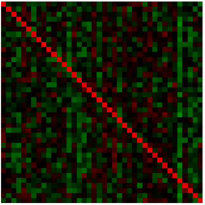
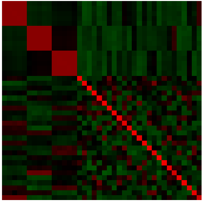
Figure 3: Heat maps of the sample covariance matrices. Examples 1 (top left) and 3 (top right) do not have a block-diagonal structure, whereas examples 2 (bottom left) and 4 (bottom right) do.

Table 2 shows the results of common penalized regression methods on the above examples: the median MSE, median false positive and false negative rates. The component lasso performs well in all examples, including the ones where the data is not generated according to a covariance matrix with a block structure. The MSE achieved by the component lasso is the lowest. The use of the estimated connected components introduces a more significant improvement in example 2 when the signal variables are in the same component, and in example 4 (indicated by a *). The model for both of these datasets has a block-diagonal covariance matrix, where certain components contain only signal variables, and the remaining components contain only noise variables. The NNLS reweighting step helps select the components containing the signal predictors.

Method	Median MSE	Median FP	Median FN
Example 1
Lasso	2.44 (0.28)	0.50 (0.02)	0 (0.02)
Rescaled Lasso	2.16 (0.26)	0.40 (0.02)	0 (0.02)
Lasso-OLS Hybrid	2.10 (0.25)	0.25 (0.02)	0 (0.01)
Naive Elastic Net	2.17 (0.26)	0.50 (0.02)	0 (0.02)
Elastic Net	1.82 (0.25)	0.50 (0.02)	0 (0.02)
Ridge	2.79 (0.28)	0.62 (0)	0 (0)
Component Lasso	1.59 (0.22)	0.40 (0.02)	0 (0.02)
Example 2 (Signal in $C_{1}$ and $C_{2}$)
Lasso	7.63 (0.55)	0.37 (0.02)	0 (0.02)
Rescaled Lasso	7.17 (0.58)	0.33 (0.02)	0 (0.02)
Lasso-OLS Hybrid	7.48 (0.58)	0.25 (0.02)	0.2 (0.02)
Naive Elastic Net	6.08 (0.48)	0.43 (0.01)	0 (0.02)
Elastic Net	5.87 (0.40)	0.50 (0.01)	0 (0.02)
Ridge	6.61 (0.47)	0.50 (0)	0 (0)
Component Lasso	4.89 (0.33 )	0.43 (0.01)	0 (0.02)
Example 2 (Signal in $C_{1}$)
Lasso	5.95 (0.53)	0.25 (0.02)	0 (0.02)
Rescaled Lasso	5.49 (0.44)	0.20 (0.02)	0 (0.02)
Lasso-OLS Hybrid	5.31 (0.47)	0 (0.01)	0.2 (0.01)
Naive Elastic Net	4.14 (0.47)	0.33 (0.01)	0 (0.01)
Elastic Net	1.83 (0.27)	0 (0.02)	0 (0)
Ridge	4.4 (0.5)	0.50 (0)	0 (0)
Component Lasso	1.57* (0.27)	0 (0.02)	0 (0)
Example 3
Lasso	58.61 (1.43)	0.31 (0.01)	0.23 (0.01)
Rescaled Lasso	58.44 (1.54)	0.31 (0.01)	0.25 (0.01)
Lasso-OLS Hybrid	57.25 (1.64)	0.28 (0.01)	0.24 (0.01)
Naive Elastic Net	38.74 (0.93)	0.41 (0)	0.14 (0.01)
Elastic Net	31.75 (0.69)	0.46 (0)	0 (0.02)
Ridge	32.86 (0.74)	0.50 (0)	0 (0)
Component Lasso	31.16 (0.73)	0.46 (0)	0 (0.02)
Example 4
Lasso	46.62 (3.29)	0.60 (0.01)	0.37 (0.01)
Rescaled Lasso	28.67 (3.09)	0.29 (0.02)	0.31 (0)
Lasso-OLS Hybrid	15.75 (2.02)	0 (0.01)	0.32 (0.02)
Naive Elastic Net	44.90 (3.01)	0.47 (0.01)	0.20 (0.01)
Elastic Net	23.79 (2.66)	0.25 (0.03)	0 (0.01)
Ridge	61.74 (3.99)	0.62 (0)	0 (0)
Component Lasso	10.74* (2.34)	0.06 (0.01)	0.04 (0.01)

Table 2: Median MSE, false positive and false negative rates for the four simulated examples using 7 regression methods. Numbers in parentheses are the standard errors.

For every data set, the connected-component split which gave the lowest validation MSE is chosen to compute the test error. Tables 2-6 show the distribution of the number of components that minimize the error in all examples. The number of components (NOC) by itself is not an appropriate measure to verify how the predictors are being grouped. For example, consider the case where some of the connected components only contain noise variables. Then, whether those variables are grouped correctly or kept in one big component does not affect the performance of the component lasso as long as the noisy components are excluded. In order to focus on how the signal variables are split, we use the misclassification measure from CT2005 on the signal variables only:

$$M(C,T)=\frac{\sum_{i>i^{\prime}}|I_{C}(i,i^{\prime})-I_{T}(i,i^{\prime})|}{{n\choose 2}},$$

where C is the partition of points, T corresponds to the true clustering, and $I()$ is an indicator function for whether the clustering places i and i’ in the same cluster. The measure quantifies the misclassification of signal variables over all signal pairs. It can be seen from the tables that the component lasso method favors splitting the predictors into clusters with low misclassification rate. The true number of components, which corresponds to the number of diagonal blocks in the covariance matrix used to generate the data, is indicated by a *.

Number of Components	1*	3	5	7
Number of Datasets	38	26	21	15
Mis. Rate	0	0.60	0.86	1

Table 3: Example 1: Optimal NOC and misclassification rate of the signal variables.

N. of Components	1	2*	3	4	5	6	7	8
N. of Datasets	35	14	6	6	9	12	12	6
Mis. Rate	0.67	0	0.17	0.20	0.18	0.25	0.28	0.33

Table 4: Example 2 (Signal in $C_{1}$ and $C_{2}$): Optimal NOC and misclassification rate of the signal variables.

N. of Components	1	2*	3	4	5	6	7	8
N. of Datasets	45	11	16	8	10	8	2	0
Mis. Rate	0	0	0.43	0.63	0.55	0.71	0.92	-

Table 5: Example 2 (Signal in $C_{1}$): Optimal NOC and misclassification rate of the signal variables.

N. of Components	1*	5	9	13	17	21	25
N. of Datasets	59	18	13	5	3	1	1
Mis. Rate	0	0.32	0.65	0.88	0.89	0.98	0.95

Table 6: Example 3: Optimal NOC and misclassification rate of the signal variables.

N. of Components	1	5	9	13	17	21	25	29*	33	37
N. of Datasets	20	28	14	2	3	1	2	15	11	4
Mis. Rate	0.71	0.07	0.03	0	0	0	0	0.04	0.16	0.25

Table 7: Example 4: Optimal NOC and misclassification rate of the signal variables. The true NOC is 28. 29 is the closest value in the tested grid.

3.2 Real data example

The component lasso is designed for settings where the data consist of a large number of predictors which can be split into highly correlated subgroups. We use a dataset from genetics to evaluate the performance of the method, because data in this area tend to follow this structure. Molecular markers are fragments of DNA associated with certain locations in the genome. In recent years, the abundance of molecular markers has made it possible to use them to predict genetic traits using linear regression. The genetic value of genes that influence a trait of interest is defined as the average phenotypic value over individuals with that trait. A standard genetic model consists in writing the phenotype $y$ as a sum of genetic values such that $y=X\beta+\epsilon$, where $X$ contains genetic values of the considered molecular markers.

Here, we consider the wheat data set studied in [GYp2010]. The aim is to predict genetic values of a quantitative trait, specifically grain yield in a fixed type of environment. The dataset consists of 599 observations, each corresponding to a different wheat line. Following the analysis done in [GYp2010], we use 1279 predictors which indicate the presence or absence of molecular markers. The grain yield response is available in 4 distinct environments. We normalize the data so that the predictors are centered and scaled, and the response is centered. We then split the available observations into equally sized training and test sets. Finally, we apply cross validation to determine the model parameters.

The test MSE is defined as $\sum_{i}(y_{i}-\hat{y}_{i})^{2}/n$ for $i$ in the test set. We compare the error rates of the lasso, naive elastic net, elastic net and the component lasso. We fix the range of the number of components for the component lasso to be between 1 and 50. Table 8 contains the test MSE achieved by the different methods to predict grain yield in 4 environments.

Method	Test MSE	Parameters	Variables Selected
Environment 1
Lasso	0.8547	$\lambda=5.1e^{-2}$	45
Naive Elastic Net	0.9656	$\alpha=0.05$, $\lambda=2.43e^{-4}$	1195
Elastic Net	0.9122	$\alpha=0.05$, $\lambda=9.58e^{-4}$	1151
Component Lasso	0.7552	$\alpha=0.05$, $\lambda=1.8e^{-4}$, $noc=29$	548
Environment 2
Lasso	0.8875	$\lambda=6.18e^{-3}$	38
Naive Elastic Net	1.1104	$\alpha=0.05$, $\lambda=2.68e^{-4}$	1191
Elastic Net	1.0722	$\alpha=0.05$, $\lambda=6.57e^{-4}$	1170
Component Lasso	0.8775	$\alpha=0.05$, $\lambda=2.45e^{-5}$, $noc=37$	564
Environment 3
Lasso	0.8216	$\lambda=7.23e^{-3}$	28
Naive Elastic Net	1.1087	$\alpha=0.05$, $\lambda=4.89e^{-4}$	1170
Elastic Net	1.1249	$\alpha=0.05$, $\lambda=1.20e^{-3}$	1125
Component Lasso	0.8830	$\alpha=0.05$, $\lambda=1.62e^{-3}$, $noc=17$	303
Environment 4
Lasso	0.8068	$\lambda=6.8e^{-3}$	27
Naive Elastic Net	1.0487	$\alpha=0.05$, $\lambda=5.18e^{-4}$	1157
Elastic Net	0.9349	$\alpha=0.05$, $\lambda=2.75e^{-3}$	1081
Component Lasso	0.8200	$\alpha=0.05$, $\lambda=3.36e^{-5}$, $noc=33$	564

Table 8: Test MSE, parameters, and number of non-zero predictors for the real data set.

The component lasso achieves the lowest test MSE in environments 1 and 2 by splitting the variables into 29 and 37 connected components respectively. The lasso achieves the lowest MSE in environments 3 and 4. In this dataset, splitting the genomic markers into correlated groups helped improve the accuracy in certain environments. Sorting the predictors according to the connected components chosen by the component lasso and plotting the heat map of the sample covariance matrix reveals the block-diagonal structure of the genomic markers. The corresponding connected components can be seen in Figure 4.

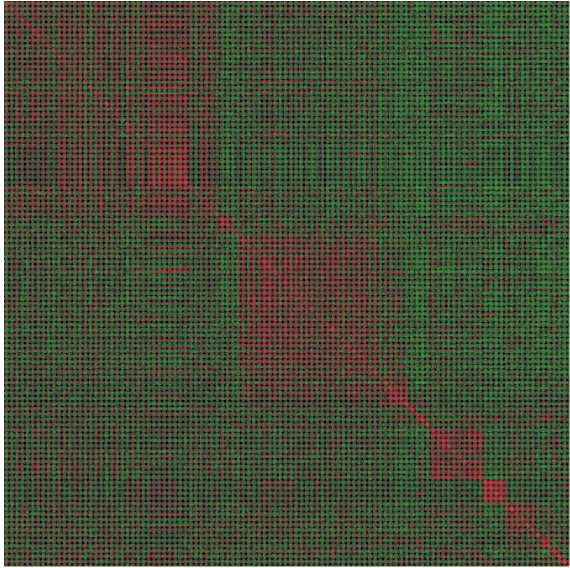
Figure 4: Heat map of the sample covariance matrix corresponding to the wheat data.

This example illustrates that the component lasso can provide improved prediction accuracy and interpretability in some real data problems.

3.3 Recovery of the true non-zero parameter support

There has been much study of the ability of the lasso and related procedures to recover the correct model, as $n$ and $p$ grow. Examples of this work include KF2000, GR2004, tropp2004, donoho2006, Mein2007, MB2006, tropp2006, ZY2006, wainwright2006, and BTW2007.

Many of the results in this area assume an “irrepresentability” condition on the design matrix of the form

$$||({X_{\cal S}}^{T}X_{\cal S})^{-1}{X_{{\cal S}}}^{T}X_{{\cal S}^{c}}{\rm sign}(\beta_{1})||_{\infty}\leq(1-\epsilon)\;\mbox{for some}\;\epsilon\in(0,1]$$ (11)

[ZY2006]. The set ${\cal S}$ indexes the subset of features with non-zero coefficients in the true underlying model, and $X_{\cal S}$ are the columns of $X$ corresponding to those features. Similarly ${\cal S}^{c}$ are the features with true coefficients equal to zero, and $X_{{\cal S}^{c}}$ the corresponding columns. The vector $\beta_{1}$ denotes the coefficients of the non-zero signal variables. The condition (11) says that the least squares coefficients for the columns of $X_{{\cal S}^{c}}$ on $X_{\cal S}$ are not too large, that is, the “good” variables ${\cal S}$ are not too highly correlated with the nuisance variables ${\cal S}^{c}$.

Now suppose that the signal variables and noise variables fall into two separate components $C_{1},C_{2}$ with sufficient within-component correlation that we are able to identify them from the data. Note that $C_{1}$ might also contain some noise variables. Then in order to recover the signal successfully, we need only that the noise variables within $C_{1}$ are irrepresentable by the signal variables, as opposed to all noise variables. This result follows from the fact that for block diagonal correlation matrices, the strong irrepresentable condition holds if and only there exists a common $0<\eta\leq 1$ for which the strong irrepresentable condition holds for every block.

3.4 Grouping effect

The grouping effect refers to the property of a regression method that returns similar coefficients for highly correlated variables. If some predictors happen to be identical, the method should return equal coefficients for the corresponding variables. The elastic net is shown to exhibit this property in the extreme case where predictors are identical ( [enet] lemma 2). Moreover, in Theorem 1 of the same paper, the authors bound the absolute value of the difference between coefficients $\hat{\beta}_{i}$ and $\hat{\beta}_{j}$ in terms of their sample correlation $\rho=x_{i}^{T}x_{j}$.

In the component lasso method, we use the elastic net or the lasso to estimate the coefficients of every connected component. If we assume that we are able to identify the components correctly from the data, then the first step of the component lasso method will preserve the grouping effect when the elastic net is used for every subproblem. NNLS fitting will also preserve the property since variables within the same connected component are scaled by the same coefficient.

4 Computational Considerations

We use the glmnet package in R for fitting the lasso and elastic net [friedman08:_regul_paths_gener_linear_model_coord_descen]. This package uses cyclical coordinate descent using a “naive” method for $p>500$ and a “covariance” mode for $p\leq 500$. Empirically, the computation time for the algorithm in naive mode scales as $O(np^{2})$ (or perhaps $O(np^{1.5})$).

Now suppose we divide the predictors into $L$ connected components: this requires $O(np^{2})$ operations and can be done without forming the sample covariance matrix $S$ (see e.g. M2002). The lasso or elastic net fitting in each of the components takes $O(Ln(p/L)^{2})=O(np^{2}/L)$. The final non-negative least squares fit can be done in $O(nL^{2})$. Thus the overall computational complexity of the component lasso is about the same as for the lasso itself.

Table 9 shows some sample timings for agglommerative clustering with different linkage methods applied to problems with different $n$ and $p$. The $p$ columns of $X$ were clustered and the code ran on a standard linux server. We used the Rclusterpp R package from the CRAN repository.

		Linkage				glmnet
n	p	ave	comp	sing	Ward
200	200	0.372	0.172	0.020	0.024	0.312
200	1000	20.698	2.852	0.268	0.412	0.056
200	2000	103.382	11.225	1.040	1.792	0.076
1000	200	1.816	0.572	0.048	0.080	0.036
2000	200	3.484	1.108	0.100	0.188	0.056
2000	1000	191.468	27.574	3.200	8.409	0.960
2000	2000	1316.306	121.244	14.765	42.722	9.453

Table 9: Timings for various hierarchical clustering techniques, compared to glmnet

We see that columns scale roughly as $O(np^{2})$, but some linkages are much faster than others. However the computational time for the lasso fit by glmnet seems to grow more slowly than that for the clustering operations.

However, there is potential for significant speedups in the component lasso algorithm. The main bottleneck is the clustering step, which requires about $O(np^{2})$ operations, as seen above. But in fact we do not need to cluster all $p$ features. If a feature is never entered into the model, we don’t need to determine its cluster membership and hence don’t need to compute its inner product with other features.

Consider for example the covariance mode of glmnet. Suppose we have a model with $k$ nonzero coefficients. For glmnet, we need to compute the inner products of these features with all other features, $kp$ in all. For the component lasso, suppose that we have $K$ clusters of equal size, and $k/K$ nonzero coefficients in each. Then we only need to compute $K(k/K)(p/K)=kp/K$ inner products, plus the number needed to determine the cluster memberships of clusters containing each of the $k$ features. This is $O(p)$ inner products. Thus the total number is reduced from $O(kp)$ to $O(kp/K+p)$. A careful implementation of this procedure will be done in future work.

We note that cross validation is potentially slower for the component lasso since it needs to consider splitting the covariance matrix into multiple numbers of components. This results in an extra parameter— the number of components— that must be varied in the cross-validation step.

Finally, the the modular structure of the component lasso lends itself naturally to parallel computation. This will also be developed in future work.

5 Discussion

In this paper we have proposed the component lasso, a penalized regression and variable selection method. In particular, we have shown that estimating and exploiting the block-diagonal structure of the sample covariance matrix— solving separate lasso problems and then recombining— can yield more accurate predictions and better recovery of the support of the signal. We provide simulated and real data examples where the component lasso outperforms standard regression methods in terms of prediction error and support recovery.

There are possible extensions of this work to other settings. Consider a $\ell_{1}$-penalized logistic regression model with outcome $y_{i}\in[0,1]$, $\mu={\rm Pr}(Y=1|x)$ and linear predictor $\eta=\log(\mu/(1-\mu))=\beta_{0}+x\beta$. Then the subgradient equations have the form

$$X^{T}WX\beta-X^{T}Wz+\lambda\cdot\text{sign}(\beta)=0$$ (12)

with $z=\beta_{0}+X\beta$ and $W={\rm diag}(\mu_{1},\mu_{2},\ldots\mu_{n})$. Typical algorithms start with some initial value $\beta^{\prime}$, compute $W$ and $z$ and then solve (12). Then $W$ and $z$ are updated and the process is repeated until convergence. This is known as iteratively reweighted (penalized) least squares (IRLS).

We see that the appropriate connected components are those of $X^{T}WX$: however this depends on $\beta$ and would have to be re-computed at each iteration. We might instead set $\beta^{\prime}=0$ so that $X^{T}WX=X^{T}X/4$. Hence we find the connected components of $X^{T}X$ and fix them. This leads to $K$ separate $\ell_{1}$-penalized logistic regression problems with estimates $\hat{\eta}_{1},\hat{\eta}_{2},\ldots\hat{\eta}_{K}$. These could be combined by a non-negative-constrained logistic regression of $y$ on $\{\hat{\eta}_{\ell},k=1,2,\ldots K\}$. An analogous approach could be used for other generalized linear models.

The component lasso achieves a significant reduction in prediction error in examples for which the covariance matrix has a block-diagonal structure and where some components only contain noise variables. The NNLS step allows the component lasso to select the relevant components due to the fact that it induces sparsity in the estimated coefficients. The component lasso also exhibits a better performance in other examples, in which NNLS helps by weighting the contribution of each component. Thus the properties of NNLS are crucial to the performance of the method. In future work we will study the theoretical properties of the component lasso.

Acknowledgements

The authors thank Trevor Hastie for helpful suggestions. Robert Tibshirani was supported by National Science Foundation Grant DMS-9971405 and National Institutes of Health Contract N01-HV-28183.

References

- [1] \harvarditemBuhlmann \harvardand Zhang2007BUH2007 Buhlmann, P., R. P. v. d. G. S. \harvardand Zhang, C.-H. \harvardyearleft2007\harvardyearright, ‘Correlated variables in regression: clustering and sparse estimation’, Journal of Statistical Planning and Inference 143, 1835–1871.
- [2] \harvarditem[Bunea et al.]Bunea, Tsybakov \harvardand Wegkamp2007BTW2007 Bunea, F., Tsybakov, A. \harvardand Wegkamp, M. \harvardyearleft2007\harvardyearright, ‘Sparsity oracle inequalities for the lasso’, Electronic Journal of Statistics 1, 169–194.
- [3] \harvarditem[Chen et al.]Chen, Donoho \harvardand Saunders1998bp Chen, S., Donoho, D. \harvardand Saunders, M. \harvardyearleft1998\harvardyearright, ‘Atomic decomposition for basis pursuit’, SIAM Journal on Scientific Computing 20(1), 33–61.
- [4] \harvarditemChipman \harvardand Tibshirani2005CT2005 Chipman, H. \harvardand Tibshirani, R. \harvardyearleft2005\harvardyearright, ‘Hybrid hierarchical clustering with applications to microarray data’, Biostatistics 7, 286–301.
- [5] \harvarditem[Crossa et al.]Crossa, de los Campos, Pe rez, Gianola, Juan Burguen and Jose Luis Araus, Dreisigacker, Yan, Arief, Banziger \harvardand Braun2010GYp2010 Crossa, J., de los Campos, G., Pe rez, P., Gianola, D., Juan Burguen and Jose Luis Araus, * Dan Makumbi, . R. P. S., Dreisigacker, S., Yan, J., Arief, V., Banziger, M. \harvardand Braun, H.-J. \harvardyearleft2010\harvardyearright, ‘Prediction of genetic values of quantitative traits in plant breeding using pedigree and molecular markers’, Genetics 186(2), 713–724.
- [6] \harvarditemDonoho2006donoho2006 Donoho, D. \harvardyearleft2006\harvardyearright, ‘For most large underdetermined systems of equations, the minimal -norm solution is the sparsest solution’, Communications on Pure and Applied Mathematics 59, 797–829.
- [7] \harvarditem[Friedman et al.]Friedman, Hastie \harvardand Tibshirani2010friedman08:_regul_paths_gener_linear_model_coord_descen Friedman, J., Hastie, T. \harvardand Tibshirani, R. \harvardyearleft2010\harvardyearright, ‘Regularization paths for generalized linear models via coordinate descent’, Journal of Statistical Software 33(1).
- [8] \harvarditemGreenshtein \harvardand Ritov2004GR2004 Greenshtein, E. \harvardand Ritov, Y. \harvardyearleft2004\harvardyearright, ‘Persistence in high-dimensional linear predictor selection and the virtue of overparametrization’, Bernoulli 10, 971–988.
- [9] \harvarditemKnight \harvardand Fu2000KF2000 Knight, K. \harvardand Fu, W. \harvardyearleft2000\harvardyearright, ‘Asymptotics for lasso-type estimators’, Annals of Statistics 28(5), 1356–1378.
- [10] \harvarditemMazumder \harvardand Hastie2012MH2012 Mazumder, R. \harvardand Hastie, T. \harvardyearleft2012\harvardyearright, ‘The graphical lasso: New insights and alternatives’, Electron. J. Statist. 6, 2125–2149.
- [11] \harvarditemMeinshausen2007Mein2007 Meinshausen, N. \harvardyearleft2007\harvardyearright, ‘Lasso with relaxation’, Computational Statistics and Data Analysis, to appear .
- [12] \harvarditemMeinshausen \harvardand Bühlmann2006MB2006 Meinshausen, N. \harvardand Bühlmann, P. \harvardyearleft2006\harvardyearright, ‘High-dimensional graphs and variable selection with the lasso’, Annals of Statistics 34, 1436–1462.
- [13] \harvarditemMurtagh2002M2002 Murtagh, F. \harvardyearleft2002\harvardyearright, Clustering in massive data sets, in Abello, James M.; Pardalos, Panos M.; Resende, Mauricio G. C., Handbook of massive data sets, Massive Computing, Springer, pp. 513–516.
- [14] \harvarditem[Park et al.]Park, Hastie \harvardand Tibshirani2007GE2007 Park, M., Hastie, T. \harvardand Tibshirani, R. \harvardyearleft2007\harvardyearright, ‘Averaged gene expressions for regression’, Biostatistics 8, 212–227.
- [15] \harvarditem[Tan et al.]Tan, Witten \harvardand Shojaie2013TWS2013 Tan, K. M., Witten, D. \harvardand Shojaie, A. \harvardyearleft2013\harvardyearright, ‘The Cluster Graphical Lasso for improved estimation of Gaussian graphical models’, ArXiv e-prints .
- [16] \harvarditemTibshirani1996lasso Tibshirani, R. \harvardyearleft1996\harvardyearright, ‘Regression shrinkage and selection via the lasso’, Journal of the Royal Statistical Society Series B 58(1), 267–288.
- [17] \harvarditemTropp2004tropp2004 Tropp, J. \harvardyearleft2004\harvardyearright, ‘Greed is good: algorithmic results for sparse approximation’, IEEE Transactions on Information Theory 50, 2231– 2242.
- [18] \harvarditemTropp2006tropp2006 Tropp, J. \harvardyearleft2006\harvardyearright, ‘Just relax: convex programming methods for identifying sparse signals in noise’, IEEE Transactions on Information Theory 52, 1030–1051.
- [19] \harvarditemWainwright2006wainwright2006 Wainwright, M. \harvardyearleft2006\harvardyearright, Sharp thresholds for noisy and high-dimensional recovery of sparsity using -constrained quadratic programming, Technical report, Department of Statistics, University of California, Berkeley.
- [20] \harvarditem[Witten et al.]Witten, Friedman \harvardand Simon2011WFS2011 Witten, D., Friedman, J. \harvardand Simon, N. \harvardyearleft2011\harvardyearright, ‘New insights and faster computations for the graphical lasso’, J. Comp. and Graph. Statist. 20, 892–200.
- [21] \harvarditemWitten \harvardand Tibshirani2009WT2009 Witten, D. \harvardand Tibshirani, R. \harvardyearleft2009\harvardyearright, ‘Covariance-regularized regression and classification for high-dimensional problems’, Journal of the Royal Statistical Society 71, 615–636.
- [22] \harvarditemZhao \harvardand Yu2006ZY2006 Zhao, P. \harvardand Yu, B. \harvardyearleft2006\harvardyearright, ‘On model selection consistency of lasso’, Journal of Machine Learning Research 7, 2541–2563.
- [23] \harvarditemZou \harvardand Hastie2005enet Zou, H. \harvardand Hastie, T. \harvardyearleft2005\harvardyearright, ‘Regularization and variable selection via the elastic net’, Journal of the Royal Statistical Society Series B 67(2), 301–320.
- [24]