Abstract

Like many other models, Composite Higgs Models feature the existence of heavy vector-like quarks. Mixing effects between the Standard Model fields and the heavy states, which can be quite large in case of the top quark, imply deviations from the SM. In this work we investigate the possibility of heavy bottom partners. We show that they can have a significant impact on electroweak precision observables and the current Higgs results if there is a sizeable mixing with the bottom quark. We explicitly check that the constraints from the measurement of the CKM matrix element $V_{tb}$ are fulfilled, and we test the compatibility with the electroweak precision observables. In particular we evaluate the constraint from the $Z$ coupling to left-handed bottom quarks. General formulae have been derived which include the effects of new bottom partners in the loop corrections to this coupling and which can be applied to other models with similar particle content. Furthermore, the constraints from direct searches for heavy states at the LHC and from the Higgs search results have been included in our analysis. The best agreement with all the considered constraints is achieved for medium to large compositeness of the left-handed top and bottom quarks.

1 Introduction

The announcement of the discovery of a new scalar particle by the LHC experiments ATLAS [1] and CMS [2] has marked a milestone in elementary particle physics. Since then, the properties of the particle have been investigated and strongly suggest it to be the Higgs boson, i.e. the particle related to the Higgs mechanism. So far no new additional particles have been discovered which could help to clarify the question which is the dynamics behind electroweak symmetry breaking (EWSB). It could be weakly interacting like in the Standard Model (SM) or in its supersymmetric extensions. The Higgs particle could also arise as pseudo Nambu-Goldstone boson (pNGB) from a strongly-coupled sector [3, 4], as is the case in Composite Higgs Models. In the Strongly-Interacting Light Higgs (SILH) [5] scenario there exists a light, narrow Higgs-like scalar, which is a bound state from some strong dynamics. Due to its Goldstone nature, the Higgs boson is separated from the other usual resonances of the strong sector by a mass gap. The low-energy particle content is the same as in the SM. In Composite Higgs Models the problem of the fermion mass generation is solved by the idea of partial compositeness [6]. The SM fermions are elementary particles which couple linearly to the heavy states of the strong sector that carry equal quantum numbers. In particular the top quark can be largely composite. The linear couplings of the SM particles to the strong sector explicitly break the global symmetry of the latter and the Higgs potential arises from loops of SM particles, with the top quark giving the main contribution. In order to naturally accommodate a low-mass Higgs boson of $\sim 125$ GeV the top partners should be rather light, with masses $\raisebox{-3.69899pt}{~{}\shortstack{$<$ \\ [-0.07cm] $\sim$}}~{}1$ TeV [7, 8, 9, 10], depending on the model and the scale of compositeness. This bound can be relaxed somewhat by contributions from new heavy gluons [11]. Heavy vector-like resonances in this mass range can be produced and searched for at the LHC [12, 13, 14].

The SILH [5] Lagrangian arises as first term of an expansion in $\xi=v^{2}/f^{2}\ll 1$, where $v$ is the scale of EWSB and $f$ is the typical scale of the strong sector. It can be used in the vicinity of the SM limit given by $\xi\to 0$. For larger values of $\xi$ a resummation of the series in $\xi$ is required. Explicit models built in five-dimensional warped space can provide such a resummation. In the Minimal Composite Higgs Model (MCHM) of Ref. [15], which is based on a 5-dimensional theory in Anti-de-Sitter space-time, the bulk symmetry $SO(5)\times U(1)_{X}\times SU(3)$ is broken down to the SM gauge group on the ultraviolet (UV) boundary and to $SO(4)\times U(1)_{X}\times SU(3)$ on the infrared (IR). The mixing effects between the SM fields and the heavy states of the new sector, which arise at tree-level, lead to sizable deviations from the SM predictions. Composite Higgs Models are therefore mainly challenged by the electroweak precision tests (EWPT) [16, 17, 18]. Particularly strong constraints can arise from the $Zb_{L}\bar{b}_{L}$ coupling, which has been measured very precisely and agrees with the SM prediction at the sub-percent level. With the top quark mixing strongly with the new sector, the left-handed bottom quark $b_{L}$ which is in the same weak doublet as $t_{L}$ receives large modifications of its couplings. The $Zb_{L}\bar{b}_{L}$ coupling is safe from large corrections if the fermions are embedded in fundamental 5 or 10 representations of $SO(5)$, where $b_{L}$ belongs to a bi-doublet (2,2) of $SU(2)_{L}\times SU(2)_{R}$, and the $SO(4)$ symmetry is enlarged to $O(4)$ [19]. Subsequent investigations including the fermion composites in full representations of the $SO(5)$ [20, 21] and extended to models with multiple sets of fermionic composites [22] showed that Composite Higgs Models can fulfill the constraints of EWSB. Further constraints on these models come from flavour physics. Four-fermion operators that arise in Composite Higgs Models contribute to flavor-changing processes and electric dipole moments. The flavour structure of the strong sector cannot be predicted through naturalness considerations, and a variety of flavour implementations can be realized [23, 24, 25, 26, 27, 28, 29, 30, 31].

The Composite Higgs couplings to the SM particles are changed with respect to the ones of the SM Higgs boson. In the MCHMs of Refs. [7, 15, 32] they can be parametrized in terms of a single parameter $\xi$. These coupling modifications change the Higgs boson phenomenology [33, 34, 35, 36, 37, 38, 39, 40, 41, 42]. With the top quark being a composite particle, mixing effects with the heavy top partners induce further changes in the top-Higgs Yukawa coupling. In addition top partners running in the loops of the loop-induced Higgs couplings to gluons and photons could lead to sizeable corrections of these vertices. It has been shown [43, 36, 40, 44, 45, 46], however, that these vertices depend on the pure non-linearities of the Higgs boson and are not sensitive to the details of the resonance spectrum. By applying the low-energy theorem (LET)[47], it can be shown that the corrections to the Yukawa coupling and the contributions from the extra fermion loops cancel each other, so that the loop-induced couplings only depend on $v/f$. The bottom quark, being the next-heaviest quark, implies a sizable mixing with the strong sector also for the bottom. In this case, due to the small bottom mass, the LET cannot be applied any more and the Higgs loop-couplings to gluons and photons will depend on the resonance structure of the strong sector, with significant implications for the Higgs phenomenology [44, 46, 48].

The aim of this paper is to study the implications of composite bottom quarks on the viability of Composite Higgs Models and on the LHC Higgs phenomenology by introducing a minimum amount of new parameters. For this purpose the fermions are embedded in the ${\bf 10}$, which is the smallest possible representation of $SO(5)$ that allows to include partial compositeness for the bottom quarks, while being compatible with the EWPTs by implementing custodial symmetry. The outline of the paper is as follows. In section 2 we present the model. In section 3 the new contributions to the electroweak precision observables due to the composite nature of the $b$-quark and to the additional heavy resonances are computed, in particular the new contributions to the loop corrections of the $Zb_{L}\bar{b}_{L}$ coupling. We then perform a $\chi^{2}$ test to investigate the compatibility of the model with the constraints that arise from electroweak precision measurements. Section 4 is devoted to the constraints from the LHC Higgs results and the direct searches for heavy fermions. In order to compare with the experimental best fit values to the Higgs rates, the Higgs production and decay processes are calculated for the model. Likewise the mass spectrum of the heavy fermion sector and the decay widths of the new resonances are computed and confronted to the LHC searches for heavy fermions. A brief discussion on implications from flavour physics is included. In section 5 we present our numerical results. The $\chi^{2}$ test taking into account the EWPTs and the newest experimental measurement of the CKM matrix element $V_{tb}$ is extended to include the latest Higgs rates reported by the experiments. Our results are summarized in the conclusions, section 6.

2 The Model

The models given in Refs. [15, 7] have been constructed in terms of five-dimensional theories on Anti-de-Sitter space-time and provide a resummation for large values of $\xi$. In the following we will work in the simplest model including custodial symmetry and allowing for the inclusion of bottom quarks as composite objects. We will show the effects of heavy bottom partners for a minimal $SO(5)\times U(1)_{X}/SO(4)\times U(1)_{X}$ symmetry breaking pattern, where the additional $U(1)_{X}$ is introduced to guarantee the correct fermion charges. The electroweak group $SU(2)_{L}\times U(1)_{Y}$ of the SM is embedded into $SO(4)\times U(1)_{X}$ with the hypercharge $Y$ given by $Y=T^{3}_{R}+X$. The coset $SO(5)/SO(4)$ provides four Goldstone bosons, three of them are the longitudinal modes of the vector bosons and one is the Higgs boson. The four Goldstone bosons can be parameterized in terms of the field

$$\Sigma=\Sigma_{0}\exp(\Pi(x)/f),\hskip 28.45274pt\Sigma_{0}=(0,0,0,0,1)\;,\hskip 28.45274pt\Pi(x)=-i\sqrt{2}T^{\hat{a}}h^{\hat{a}}(x)\;,$$ (1)

with $T^{\hat{a}}$ ($\hat{a}=1..4$) denoting the generators of the coset $SO(5)/SO(4)$. They are given by

$$(T^{\hat{a}})_{ij} =-\frac{i}{\sqrt{2}}\left(\delta^{\hat{a}}_{i}\delta^{5}_{j}-\delta^{\hat{a}}_{j}\delta^{5}_{i}\right)\;.$$ (2)

Together with the generators of the $SU(2)_{L,R}$ $(a,b,c=1,2,3,\,i,j=1,...,5)$,

$$(T^{a}_{L})_{ij} =-\frac{i}{2}\left[\frac{1}{2}\epsilon^{abc}(\delta^{b}_{i}\delta^{c}_{j}-\delta^{b}_{j}\delta^{c}_{i})+\delta^{a}_{i}\delta^{4}_{j}-\delta^{4}_{i}\delta^{a}_{j}\right]\;,$$ (3)

$$(T^{a}_{R})_{ij} =-\frac{i}{2}\left[\frac{1}{2}\epsilon^{abc}(\delta^{b}_{i}\delta^{c}_{j}-\delta^{b}_{j}\delta^{c}_{i})-\delta^{a}_{i}\delta^{4}_{j}+\delta^{4}_{i}\delta^{a}_{j}\right]\;,$$ (4)

they form the generators for the fundamental representation of $SO(5)$. This leads to the explicit expression for the Goldstone field $\Sigma$,

$$\Sigma=\frac{\sin h/f}{h}(h_{1},h_{2},h_{3},h_{4},h\cot(h/f))\;,\hskip 28.45274pth=\sqrt{\sum_{\hat{a}=1}^{4}h_{\hat{a}}^{2}}\;.$$ (5)

The low-energy physics of the strong sector can be described by a non-linear $\sigma$-model. The kinetic term of the Goldstone field can then be written as

$$\mathcal{L}_{kin}=\frac{f^{2}}{2}\left(D_{\mu}\Sigma\right)\left(D^{\mu}\Sigma\right)^{T}\;,\quad\mbox{with}\quad D_{\mu}\Sigma=\partial_{\mu}\Sigma-ig^{\prime}B_{\mu}\Sigma(T^{3}_{R}+X)-igW_{\mu}^{a}\Sigma T^{a}_{L}\;,$$ (6)

where $W_{\mu}^{a}$ and $B_{\mu}$ are the electroweak $SU(2)$ and $U(1)$ fields, respectively, with the corresponding couplings $g$ and $g^{\prime}$. In the unitary gauge the vacuum expectation value (VEV) can be aligned with the direction of $h_{4}$ which is identified with $H\equiv h_{4}$, so that

$$\Sigma=(0,0,0,\sin(H/f),\cos(H/f))\;,$$ (7)

and we get for the kinetic term

$$\mathcal{L}_{kin}=\frac{1}{2}\partial_{\mu}H\partial^{\mu}H+\frac{f^{2}}{4}\sin^{2}\left(\frac{H}{f}\right)\left[g^{2}W_{\mu}^{+}W^{\mu-}+\frac{g^{2}}{2\cos^{2}\theta_{W}}Z^{\mu}Z_{\mu}\right]\;.$$ (8)

Expanding Eq. (8) in powers of the Higgs field $H=\langle H\rangle+h$, and identifying

$$\xi=\left(\frac{v}{f}\right)^{2}=\sin^{2}\frac{\langle H\rangle}{f}\;,$$ (9)

one obtains the couplings to the gauge fields in terms of the corresponding SM couplings ($V=W,Z$)

$$g_{hVV}=g_{hVV}^{\text{SM}}\,\sqrt{1-\xi}\;,\qquad g_{hhVV}=g_{hhVV}^{\text{SM}}\,(1-2\xi)\;,$$ (10)

and the usual mass relation $m_{W}^{2}=g^{2}v^{2}/4$, with $v=1/\sqrt{G_{F}\sqrt{2}}\approx 246$ GeV.

New fermionic resonances in Composite Higgs Models are expected to be well below the cut-off of the effective theory in order to accommodate a Higgs boson with mass $m_{h}\approx 125$ GeV [8, 9, 10]. Fermion mass generation is then achieved by the principle of partial compositeness, in which an elementary fermion acquires its mass through the mixing with new vector-like fermions of the strong sector. This can be implemented in the Lagrangian through linear couplings of the elementary sector with the strong sector. The quantum numbers of the new fermion must be such that the Lagrangian is invariant under the SM gauge group. A large, phenomenologically interesting mixing occurs if the SM fermion is heavy, which makes the discussion of the third generation quarks the most interesting. Previous works, as e.g. Refs. [22, 21, 45], have studied the mass generation of the top quark through mixing, while the bottom quark was taken massless or introduced ad hoc. The purpose of this work, however, is to study the effect of bottom partners that arise when the bottom quark mass is generated by mixing with the strong sector. This cannot be achieved by introducing only a single fermion multiplet in the fundamental or spinorial representation of $SO(5)$. In the following we will therefore consider a $\text{\bf 10}_{2/3}$, which is the smallest representation of $SO(5)$ having the desired features. Note that since there is only one multiplet giving a mass both to the top and bottom quark, no new parameters need to be introduced compared to the previous models where a $\text{\bf 5}_{2/3}$ is used to generate a mass for the top quark. If there are no new resonances of the strong sector below the cut-off, apart from the Higgs boson, the model displays the same phenomenology as the one with fermions embedded in the fundamental representation, cf. Ref. [7]. The 10 of $SO(5)$ is a two-index antisymmetric representation, which can be written as follows

$$\begin{split}&\mathcal{Q}=\frac{1}{2}\\ &\begin{pmatrix}0&-(u+u_{1})&\frac{i(d-\chi)}{\sqrt{2}}+\frac{i(d_{1}-\chi_{1})}{\sqrt{2}}&\frac{d+\chi}{\sqrt{2}}-\frac{d_{1}+\chi_{1}}{\sqrt{2}}&d_{4}+\chi_{4}\\ u_{1}+u&0&\frac{d_{1}+\chi_{1}}{\sqrt{2}}+\frac{d+\chi}{\sqrt{2}}&\frac{i(d_{1}-\chi_{1})}{\sqrt{2}}-\frac{i(d-\chi)}{\sqrt{2}}&-i(d_{4}-\chi_{4})\\ -\frac{i(d_{1}-\chi_{1})}{\sqrt{2}}-\frac{i(d-\chi)}{\sqrt{2}}&-\frac{d_{1}+\chi_{1}}{\sqrt{2}}-\frac{d+\chi}{\sqrt{2}}&0&u_{1}-u&t_{4}+T_{4}\\ \frac{d_{1}+\chi_{1}}{\sqrt{2}}-\frac{d+\chi}{\sqrt{2}}&\frac{i(\chi_{1}-d_{1})}{\sqrt{2}}+\frac{i(d-\chi)}{\sqrt{2}}&u-u_{1}&0&-i(t_{4}-T_{4})\\ -d_{4}-\chi_{4}&i(d_{4}-\chi_{4})&-t_{4}-T_{4}&i(t_{4}-T_{4})&0\end{pmatrix}\end{split}$$ (11)

where the fermions $u,u_{1},t_{4}$ and $T_{4}$ have electric charge 2/3, $d,d_{1}$ and $d_{4}$ have charge -1/3, and the charge of $\chi,\chi_{1}$ and $\chi_{4}$ is 5/3.

	$u$	$u_{1}$	$t_{4}$	$T_{4}$	$d$	$d_{1}$	$d_{4}$	$\chi$	$\chi_{1}$	$\chi_{4}$
$T_{3,L}$	0	0	-1/2	1/2	-1	0	-1/2	1	0	1/2
$T^{2}_{L}$	1	0	1/2	1/2	1	0	1/2	1	0	1/2
$T_{3,R}$	0	0	1/2	-1/2	0	-1	-1/2	0	1	1/2
$T^{2}_{R}$	0	1	1/2	1/2	0	1	1/2	0	1	1/2
$Y$	2/3	2/3	7/6	1/6	2/3	-1/3	1/6	2/3	5/3	7/6

Table 1: Quantum numbers of the new vector-like fermions under $SU(2)_{L}\times SU(2)_{R}$. The last line is the hypercharge.

The decomposition of the 10 under $SU(2)_{L}\times SU(2)_{R}$ is

$$\mathbf{10}=(\mathbf{2,2})\oplus(\mathbf{3,1})\oplus(\mathbf{1,3})\;.$$ (12)

The exact quantum numbers of each of the new fermions can be read off Table 1. The Lagrangian including the new fermion multiplet $\mathcal{Q}$ then reads

$$\begin{split}\mathcal{L}=&\,i\,\text{Tr}(\bar{\mathcal{Q}}_{R}\not{D}\mathcal{Q}_{R})+i\,\text{Tr}(\bar{\mathcal{Q}}_{L}\not{D}\mathcal{Q}_{L})+i\bar{q}_{L}\not{D}q_{L}+i\bar{b}_{R}\not{D}b_{R}+i\bar{t}_{R}\not{D}t_{R}\\ &-M_{10}\text{Tr}(\bar{\mathcal{Q}}_{R}\mathcal{Q}_{L})-yf\left(\Sigma^{\dagger}\bar{\mathcal{Q}}_{R}\mathcal{Q}_{L}\Sigma\right)+h.c.\\ &-\lambda_{t}\bar{t}_{R}u_{1L}-\lambda_{b}\bar{b}_{R}d_{1L}-\lambda_{q}(\bar{T}_{4R},\bar{d}_{4R})q_{L}+h.c.\;,\end{split}$$ (13)

where the SM doublet of the left-handed top and bottom quark is denoted by $q_{L}$ and the right-handed top (bottom) quark by $t_{R}$ ($b_{R}$). The covariant derivative acts on $\mathcal{Q}$ as

$$D_{\mu}\mathcal{Q}=\partial_{\mu}\mathcal{Q}-igW^{a}[T^{a}_{L},\mathcal{Q}]-ig^{\prime}B\big{(}[T^{3}_{R},\mathcal{Q}]+X\mathcal{Q}\big{)}\;,\hskip 28.45274ptX=(2/3)\mathds{1}\;,$$ (14)

with the generators $T^{a}_{L}$ defined as in Eq. (3). Note that the mixing terms with the coupling constants $\lambda_{q}$,$\lambda_{t}$ and $\lambda_{b}$ explicitly break $SO(5)$. Using the abbreviations

$$s_{H}\equiv\sin(H/f)\;,\qquad c_{H}\equiv\cos(H/f)$$ (15)

and

$$\tilde{m}_{a}\equiv\frac{1}{4}fys_{H}^{2}+M_{10}\;,\hskip 28.45274pt\tilde{m}_{b}\equiv\frac{1}{2}fy(1-\frac{1}{2}s_{H}^{2})+M_{10}\;,\hskip 28.45274pt\tilde{m}_{c}\equiv\frac{1}{2}fyc_{H}^{2}+M_{10}\;,$$ (16)

the terms of the Lagrangian in Eq. (13), which are bilinear in the quark fields, can be written as

$$-\mathcal{L}_{m_{t}}=\overline{\left(\begin{array}[]{c}t_{L}\\ u_{L}\\ u_{1L}\\ t_{4L}\\ T_{4L}\end{array}\right)}\left(\begin{array}[]{ccccc}0&0&0&0&\lambda_{q}\\ 0&\tilde{m}_{a}&-\frac{1}{4}fys_{H}^{2}&-\frac{1}{4}fyc_{H}s_{H}&-\frac{1}{4}fyc_{H}s_{H}\\ \lambda_{t}&-\frac{1}{4}fys_{H}^{2}&\tilde{m}_{a}&\frac{1}{4}fyc_{H}s_{H}&\frac{1}{4}fyc_{H}s_{H}\\ 0&-\frac{1}{4}fyc_{H}s_{H}&\frac{1}{4}fyc_{H}s_{H}&\tilde{m}_{b}&-\frac{1}{4}fys_{H}^{2}\\ 0&-\frac{1}{4}fyc_{H}s_{H}&\frac{1}{4}fyc_{H}s_{H}&-\frac{1}{4}fys_{H}^{2}&\tilde{m}_{b}\end{array}\right)\left(\begin{array}[]{c}t_{R}\\ u_{R}\\ u_{1R}\\ t_{4R}\\ T_{4R}\end{array}\right)+h.c.\;,$$ (17)

$$-\mathcal{L}_{m_{b}}=\overline{\left(\begin{array}[]{c}b_{L}\\ d_{L}\\ d_{1L}\\ d_{4L}\end{array}\right)}\left(\begin{array}[]{cccc}0&0&0&\lambda_{q}\\ 0&\tilde{m}_{a}&-\frac{1}{4}fys_{H}^{2}&fy\frac{c_{H}s_{H}}{2\sqrt{2}}\\ \lambda_{b}&-\frac{1}{4}fys_{H}^{2}&\tilde{m}_{a}&-fy\frac{c_{H}s_{H}}{2\sqrt{2}}\\ 0&fy\frac{c_{H}s_{H}}{2\sqrt{2}}&-fy\frac{c_{H}s_{H}}{2\sqrt{2}}&\tilde{m}_{c}\end{array}\right)\left(\begin{array}[]{c}b_{R}\\ d_{R}\\ d_{1R}\\ d_{4R}\end{array}\right)+h.c.\;,$$ (18)

and

$$-\mathcal{L}_{m_{\chi}}=\overline{\left(\begin{array}[]{c}\chi_{L}\\ \chi_{1L}\\ \chi_{4L}\end{array}\right)}\left(\begin{array}[]{ccc}\tilde{m}_{a}&-\frac{1}{4}fys_{H}^{2}&fy\frac{c_{H}s_{H}}{2\sqrt{2}}\\ -\frac{1}{4}fys_{H}^{2}&\tilde{m}_{a}&-fy\frac{c_{H}s_{H}}{2\sqrt{2}}\\ fy\frac{c_{H}s_{H}}{2\sqrt{2}}&-fy\frac{c_{H}s_{H}}{2\sqrt{2}}&\tilde{m}_{c}\end{array}\right)\left(\begin{array}[]{c}\chi_{R}\\ \chi_{1R}\\ \chi_{4R}\end{array}\right)+h.c.\;.$$ (19)

The mass matrices $M_{t}$, $M_{b}$ and $M_{\chi}$ can be obtained by replacing the Higgs field in Eqs. (17)-(19), encoded in $s_{H}$ and $c_{H}$, respectively, with its VEV, i.e. $H\to\langle H\rangle$. They are diagonalized by a bi-unitary transformation

$$\left(U_{L}^{(t/b/\chi)}\right)^{\dagger}M_{(t/b/\chi)}U_{R}^{(t/b/\chi)}=M_{(t/b/\chi)}^{diag}\;,$$ (20)

where $U_{L,R}^{(t/b/\chi)}$ denote the transformations that diagonalize the mass matrix in the top, bottom and charge-5/3 ($\chi$) sector, respectively. In our analysis we diagonalize them numerically, setting the values of $\lambda_{t}$ and $\lambda_{b}$ such that the physics values of the top and bottom quark masses are recovered. An analytic understanding of the size of the masses can be obtained before electroweak symmetry breaking, i.e. for $v=0$. The following rotations diagonalize the mass matrices

$$\begin{array}[]{lllll}\begin{pmatrix}q_{L}\\ Q_{L}\end{pmatrix}&\to&\begin{pmatrix}\cos\phi_{L}&\sin\phi_{L}\\ -\sin\phi_{L}&\cos\phi_{L}\end{pmatrix}&\begin{pmatrix}q_{L}\\ Q_{L}\end{pmatrix}\,,&\hskip 28.45274pt\tan\phi_{L}=\lambda_{q}/(M_{10}+fy/2)\;,\\[11.38092pt] \begin{pmatrix}t_{R}\\ u_{1R}\end{pmatrix}&\to&\begin{pmatrix}\cos\phi_{Rt}&\sin\phi_{Rt}\\ -\sin\phi_{Rt}&\cos\phi_{Rt}\end{pmatrix}&\begin{pmatrix}t_{R}\\ u_{1R}\end{pmatrix}\,,&\hskip 28.45274pt\tan\phi_{Rt}=\lambda_{t}/M_{10}\;,\\[11.38092pt] \begin{pmatrix}b_{R}\\ d_{1R}\end{pmatrix}&\to&\begin{pmatrix}\cos\phi_{Rb}&\sin\phi_{Rb}\\ -\sin\phi_{Rb}&\cos\phi_{Rb}\end{pmatrix}&\begin{pmatrix}b_{R}\\ d_{1R}\end{pmatrix}\,,&\hskip 28.45274pt\tan\phi_{Rb}=\lambda_{b}/M_{10}\;,\end{array}$$ (24)

with $Q_{L}=(T_{4L},d_{4L})$. The masses of the top partners are then found to be

$$M_{10}\,,\quad\frac{M_{10}}{\cos\phi_{Rt}}\,,\quad M_{10}+\frac{fy}{2}\,,\quad\frac{M_{10}+\frac{fy}{2}}{\cos\phi_{L}}\;,$$ (25)

and the masses of the bottom partners

$$M_{10}\,,\quad\frac{M_{10}}{\cos\phi_{Rb}}\,,\quad\frac{M_{10}+\frac{fy}{2}}{\cos\phi_{L}}\;.$$ (26)

If the new scale $f$ is much larger than $v$ an expansion in $v/f$ of the mass matrices can be performed. At leading order in $v/f$, this yields for the top and bottom quark mass

$$m_{top}=\frac{y\;v}{4}\sin\phi_{L}\sin\phi_{Rt}\;,\hskip 28.45274ptm_{bot}=\frac{y\;v}{2\sqrt{2}}\sin\phi_{L}\sin\phi_{Rb}\;.$$ (27)

We see, that in order to achieve the experimentally measured value of the top quark, $t_{L}$ and $t_{R}$ cannot be too elementary at the same time. Furthermore, as the top and bottom quark are in the same doublet, the compositeness of the left-handed bottom is directly connected to the compositeness of the left-handed top. As $\sin\phi_{L}$ cannot be too small in order to reproduce the top quark mass, this implies that the right-handed component of the bottom quark is mostly elementary, so that a small enough bottom mass can be achieved. The first correction term to the top and bottom partner masses is of $\mathcal{O}(v^{2}/f^{2})$. For the charge-$5/3$ fermions the masses can be computed analytically even for non-vanishing $v$. They are given by

$$M_{10}\,,\quad M_{10}\,,\quad M_{10}+\frac{fy}{2}\;.$$ (28)

The Higgs coupling matrices can be obtained from Eqs. (17)-(19) by expanding the mass matrices in the interaction eigenstates up to first order in the Higgs field $H$. They read

$$-\mathcal{L}_{ht\bar{t}}=y\;h\overline{\left(\begin{array}[]{c}t_{L}\\ u_{L}\\ u_{1L}\\ t_{4L}\\ T_{4L}\end{array}\right)}\underbrace{\left(\begin{array}[]{ccccc}0&0&0&0&0\\ 0&\frac{1}{2}s_{H}c_{H}&-\frac{1}{2}s_{H}c_{H}&\frac{1}{4}(2s_{H}^{2}-1)&\frac{1}{4}(2s_{H}^{2}-1)\\ 0&-\frac{1}{2}s_{H}c_{H}&\frac{1}{2}s_{H}c_{H}&\frac{1}{4}(1-2s_{H}^{2})&\frac{1}{4}(1-2s_{H}^{2})\\ 0&\frac{1}{4}(2s_{H}^{2}-1)&\frac{1}{4}(1-2s_{H}^{2})&-\frac{1}{2}s_{H}c_{H}&-\frac{1}{2}s_{H}c_{H}\\ 0&\frac{1}{4}(2s_{H}^{2}-1)&\frac{1}{4}(1-2s_{H}^{2})&-\frac{1}{2}s_{H}c_{H}&-\frac{1}{2}s_{H}c_{H}\end{array}\right)}_{G_{ht\bar{t}}/y}\left(\begin{array}[]{c}t_{R}\\ u_{R}\\ u_{1R}\\ t_{4R}\\ T_{4R}\end{array}\right)_{H=\langle H\rangle}+h.c.\;,$$ (29)

$$-\mathcal{L}_{hb\bar{b}}=y\;h\overline{\left(\begin{array}[]{c}b_{L}\\ d_{L}\\ d_{1L}\\ d_{4L}\end{array}\right)}\underbrace{\left(\begin{array}[]{cccc}0&0&0&0\\ 0&\frac{1}{2}s_{H}c_{H}&-\frac{1}{2}s_{H}c_{H}&\frac{1}{2\sqrt{2}}(1-2s_{H}^{2})\\ 0&-\frac{1}{2}s_{H}c_{H}&\frac{1}{2}s_{H}c_{H}&\frac{1}{2\sqrt{2}}(2s_{H}^{2}-1)\\ 0&\frac{1}{2\sqrt{2}}(1-2s_{H}^{2})&\frac{1}{2\sqrt{2}}(2s_{H}^{2}-1)&-s_{H}c_{H}\end{array}\right)}_{G_{hb\bar{b}}/y}\left(\begin{array}[]{c}b_{R}\\ d_{R}\\ d_{1R}\\ d_{4R}\end{array}\right)_{H=\langle H\rangle}+h.c.\;.$$ (30)

The matrices for the couplings to top-like states, $G_{ht\bar{t}}$, and to bottom-like states, $G_{hb\bar{b}}$, in the mass eigenstate basis are obtained by multiplication with the matrices $U_{L,R}$ defined in Eq. (20). The charge-5/3 fermions only interact with the Higgs boson through small off-diagonal terms and are not relevant for our analysis. Their coupling matrix is therefore not given explicitly here. The couplings of the fermions to the gauge bosons are obtained from Eq. (14) in the interaction basis with subsequent rotation to the mass eigenstates. In the following section also the couplings of the fermions to the Goldstone bosons will be needed. They can be derived from Eq. (13) by using Eq. (5) and doing the following replacements,

$$h_{1}\to\frac{G^{-}-G^{+}}{i\sqrt{2}},\hskip 28.45274pth_{2}\to-\frac{G^{-}+G^{+}}{\sqrt{2}},\hskip 28.45274pth_{3}\to G_{0}\;.$$ (31)

The couplings of the Goldstone bosons with the fermions can be found in Appendix A.

3 Computation of electroweak precision observables

The results obtained at LEP put important constraints on New Physics models. The data indirectly constrains physics at high energies which enters in loop corrections to the observables at the electroweak scale. In this section the contributions to the Peskin-Takeuchi $S$ and $T$ parameters [51] will be shortly reviewed. Subsequently, the computation of the one-loop contributions to the non-oblique corrections to the $Zb_{L}\bar{b}_{L}$ vertex due to the partial compositeness of the bottom quark will be presented. The $U$ parameter will not be discussed here, as it only receives contributions from operators of dimension eight or higher. For convenience, we use instead of $S$, $T$ and the shift in the $Zb_{L}\bar{b}_{L}$ coupling the parameters $\epsilon_{1},\epsilon_{2},\epsilon_{3}$ and $\epsilon_{b}$ [52], as they do not depend on a reference point in the SM.

3.1 Contributions to $\epsilon_{1}$

The $T$ parameter – or equivalently $\epsilon_{1}$ – gets a correction due to modified Higgs-vector boson couplings. They prevent a full cancellation of the UV-divergencies in the $T$-parameter so that a logarithmically divergent part remains [17]. It is cut off by the mass of the first vector resonance $m_{\rho}$,

$$\Delta\epsilon_{1}^{IR}=-\frac{3\alpha(m_{Z}^{2})}{16\pi\cos^{2}\theta_{W}}\xi\log\left(\frac{m_{\rho}^{2}}{m_{h}^{2}}\right)\;,$$ (32)

with $\xi=v^{2}/f^{2}$, cf. Eq. (9) and $\alpha$ the electromagnetic coupling at the scale $m_{Z}$. The Weinberg angle is denoted by $\theta_{W}$. Another important contribution to $\epsilon_{1}$ comes from loops of fermionic partners. Explicit formulae at the one-loop order can be found in Refs.[53, 22].

3.2 Contributions to $\epsilon_{3}$

Similar to the IR contribution to $\epsilon_{1}$, a UV-divergent contribution due to modified Higgs-vector boson couplings also arises for the $S$ parameter – or $\epsilon_{3}$ –,

$$\Delta\epsilon_{3}^{IR}=\frac{\alpha(m_{Z}^{2})}{48\pi\sin^{2}\theta_{W}}\xi\log\left(\frac{m_{\rho}^{2}}{m_{h}^{2}}\right)\;.$$ (33)

Additionally, at tree-level there is a UV contribution from the mixing of elementary gauge fields with new vector and axial vector resonances [5, 54],

$$\Delta\epsilon_{3}^{UV}=\frac{m_{W}^{2}}{m_{\rho}^{2}}\left(1+\frac{m_{\rho}^{2}}{m_{a}^{2}}\right)\;,$$ (34)

where $m_{a}$ denotes the mass of the first axial vector resonance. For definiteness, we set $m_{\rho}/m_{a}\approx 3/5$ as obtained in the five-dimensional $SO(5)/SO(4)$ models of Refs. [15, 7]. We explicitly checked that varying $m_{\rho}/m_{a}$ between 1 and 2 has only a slight effect on our numerical results. The finite fermionic one-loop contributions to $\epsilon_{3}$, which can be found in Ref. [53], are neglected, as they are small compared to the tree-level UV contributions given in [22]. As recently pointed out in Ref. [55], however, there can be an additional logarithmically divergent contribution stemming from fermion loops, which is given by

$$\Delta\epsilon_{3}^{div}\sim\text{Tr}\left[W_{L}^{\dagger}Y_{L}+W_{R}^{\dagger}Y_{R}\right]\;,$$ (35)

where $W_{L,R}$ are the left- and right-handed fermion couplings to $W^{3}_{\mu}$ and $Y_{L,R}$ the corresponding hypercharges. In our case the trace in Eq. (35) is zero.

3.3 Contributions to $\epsilon_{b}$

Since light quarks are assumed to couple to any New Physics in a subdominant way, no vertex corrections to the $e^{+}e^{-}$ annihilation process at LEP have to be taken into account. The only exception is the $Zb_{L}\bar{b}_{L}$ vertex, because the left-handed $b$-quark is in the same $SU(2)_{L}$ doublet as the top quark, which itself has a large mixing with composite fermions. For this vertex, New Physics contributions can thus be sizeable.

The Lagrangian for the coupling of a $Z$ boson to a quark $\Psi_{i}^{Q}$ of charge $Q$ in the mass eigenstate basis is parameterized by

$$\mathcal{L}_{Z}=\frac{g}{2c_{W}}Z_{\mu}\bar{\Psi}_{Q}^{i}\gamma^{\mu}\left(X_{ij}^{QL}P_{L}+X_{ij}^{QR}P_{R}-2s_{W}^{2}Q\delta_{ij}\right)\Psi_{Q}^{j}\;,$$ (36)

where $i,j$ run over all quarks present in the model. Here and below we use the short-hand notation $c_{W}\equiv\cos\theta_{W}$ and $s_{W}\equiv\sin\theta_{W}$. We keep the coupling general so that the result can also be applied to other cases. The decay amplitude of the $Z$ boson into a pair of massless left-handed $b$-quarks is given by

$$\mathcal{M}_{Z\to b_{\scriptscriptstyle L}\bar{b}_{\scriptscriptstyle L}}=-\frac{e(g_{b_{L}}^{SM}+\delta g_{b_{L}})}{c_{W}s_{W}}\epsilon_{\mu}(p_{Z})\bar{b}(p_{\bar{b}})\gamma^{\mu}\frac{1-\gamma_{5}}{2}b(p_{b})\;,$$ (37)

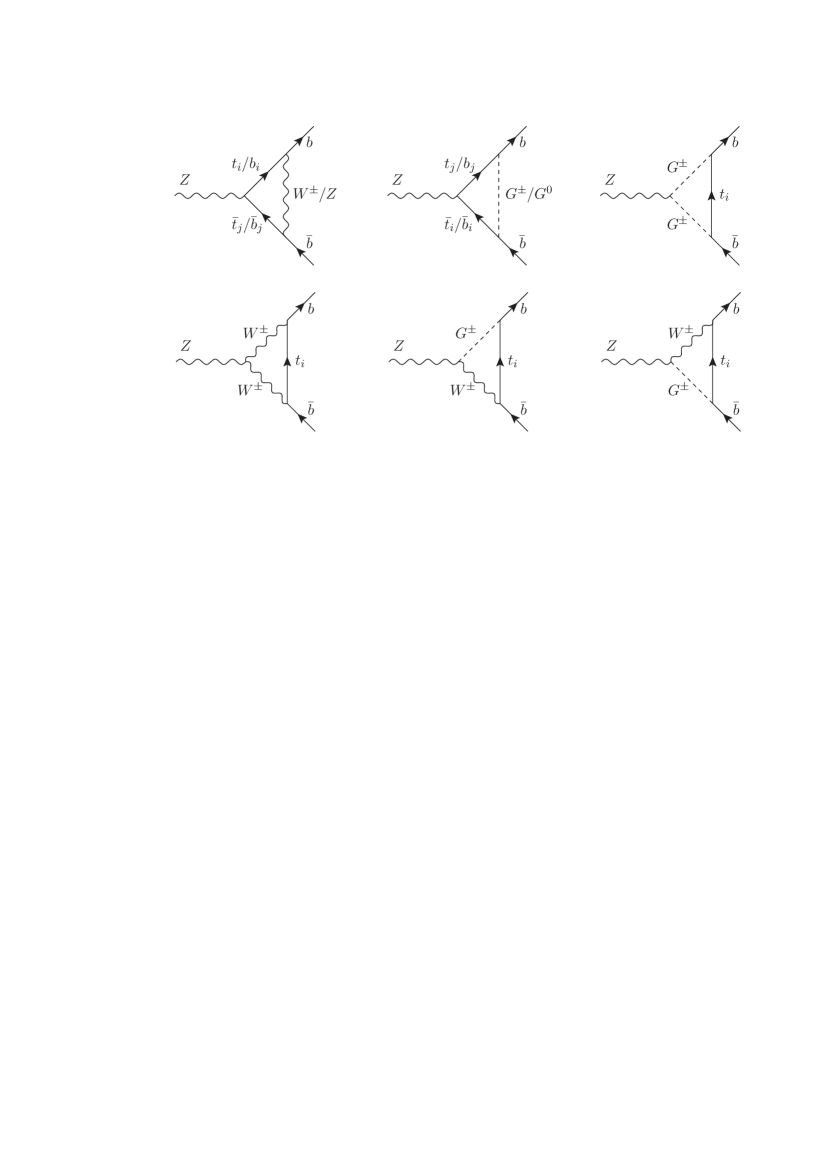
with the electric charge $e$ and the SM coupling $g_{b_{L}}^{SM}$ of the $Z$ boson to the left-handed $b$-quarks. The polarization vector of the $Z$ boson with four-momentum $p_{Z}$ is denoted by $\epsilon_{\mu}$. A left-right symmetry prevents $\delta g_{b_{L}}$, which contains the effects from New Physics, from getting tree-level contributions [19]. However, important contributions to $\delta g_{b_{L}}$ can occur through loops of new fermions. In Fig. 1 the Feynman diagrams for the one-loop corrections to $Zb_{L}\bar{b}_{L}$ including gauge bosons and Goldstone bosons are shown. There are also diagrams involving the Higgs boson, which, however, have a negligibly small contribution.

Figure 1: Loop vertex diagrams for heavy fermion partner contributions to the $Zb_{L}\bar{b}_{L}$ coupling.

In order to quantify the beyond the SM effect of the heavy quarks on $\delta g_{b_{L}}$, the SM contribution $\mathcal{M}^{t+b}_{SM}$ of the bottom and top quarks has to be subtracted,

$$\delta g_{b_{L}}=\mathcal{M}^{heavy}-\mathcal{M}^{t+b}_{SM}\;,$$ (38)

where $\mathcal{M}^{heavy}$ denotes the contributions from the loops with the heavy quarks, the top and the bottom quark. The $Zb_{L}\bar{b}_{L}$ vertex needs to be renormalized to become finite. We adopt an on-shell renormalization scheme similar to Ref. [56]. The wave function renormalization constants $\delta Z^{L,R}$ relate the left- and right-handed bare fields $b_{0}^{L,R}$ with the renormalized ones $b^{L,R}$,

$$b_{0}^{L,R}=(1+\frac{1}{2}\delta Z^{L,R})b^{L,R}\;.$$ (39)

The $Z$ boson coupling to the left-handed bottom-type quarks is proportional to, cf. Eq. (36),

$$X^{-1/3,L}=U_{L}^{b\;\dagger}T_{L}^{3}U_{L}^{b}\;,$$ (40)

where $T_{L}^{3}$ is the generator defined in Eq. (3). For the renormalization of the mixing matrix $U^{b}_{L}$ in Eq. (40) a counterterm $\delta u_{L}^{b}$ is introduced. The complete $Zb_{L}\bar{b}_{L}$ vertex including the counterterm in the mass eigenstate basis then reads

$$\begin{split}\mathcal{L}_{Z\bar{b}_{L}b_{L}}=-&\frac{e}{s_{W}c_{W}}\bar{b}\,\gamma_{\mu}\left(1+\frac{1}{2}\delta Z_{L}^{\dagger}\right)\left(1+\delta u_{L}^{b}\right)U_{L}^{b}\left(T_{L}^{3}-2s_{W}^{2}Q\right)\\ &U_{L}^{b\;\dagger}\left(1+\delta u_{L}^{b\;\dagger}\right)\left(1+\frac{1}{2}\delta Z_{L}\right)P_{L}b\,Z^{\mu}\;,\end{split}$$ (41)

where $P_{L}=(1-\gamma_{5})/2$ denotes the left-handed projector. Note that only the wave function renormalization constants for the $b$-quark fields and the counterterm of the mixing matrix are needed, whereas the electric charge, the Weinberg angle and the wave function renormalization of the $Z$ boson are already included in the oblique parameters [51, 57], due to their universality for all $Zf\bar{f}$ vertices. The counterterm is defined antihermitian, as the bare and the renormalized mixing matrices are unitary, cf. Ref. [58],

$$\delta u_{L,ij}^{b}=\frac{1}{4}\left(\delta Z_{ij}^{L}-\delta Z_{ij}^{L\;\dagger}\right)\;.$$ (42)

Defining the structure ($P_{R}=(1+\gamma_{5})/2$)

$$\Sigma_{ij}(p^{2})=\not{p}\Sigma_{ij}^{L}(p^{2})P_{L}+\not{p}\Sigma_{ij}^{R}(p^{2})P_{R}+\Sigma_{ij}^{l}(p^{2})P_{L}+\Sigma_{ij}^{r}(p^{2})P_{R}$$ (43)

for the fermion self-energy $\Sigma$, the wave function renormalization constant $\delta Z^{L}$ for the left-handed fermion field is given by

$$\delta Z^{L}_{ij} =\frac{2}{m_{i}^{2}-m_{j}^{2}}\widetilde{\text{Re}}\left(m_{j}^{2}\Sigma^{L}_{ij}(m_{j}^{2})+m_{i}m_{j}\Sigma^{R}_{ij}(m_{j}^{2})+m_{i}\Sigma^{l}_{ij}(m_{j}^{2})+m_{j}\Sigma_{ij}^{r}(m_{j}^{2})\right) i\neq j$$ (44)

$$\delta Z^{L}_{ii} =-\widetilde{\text{Re}}\,\Sigma_{ii}^{L}(m_{i}^{2})-m_{i}\frac{\partial}{\partial p^{2}}\widetilde{\text{Re}}\left(m_{i}(\Sigma^{L}_{ii}(p^{2})+\Sigma^{R}_{ii}(p^{2}))+\Sigma^{l}_{ii}(p^{2})+\Sigma^{r}_{ii}(p^{2})\right)\lvert_{p^{2}=m_{i}^{2}} i=j\;,$$ (45)

where $\widetilde{\text{Re}}$ only takes the real part of the one-loop integrals but keeps the complex structure of the parameters. Note that in our calculation we set the bottom mass to zero, which implies that either $m_{i}$ or $m_{j}$ is zero in Eq. (44) and that $m_{i}=0$ in Eq. (45).

Figure 2: Self-energy corrections needed for the renormalization of the vertex $Zb_{L}\bar{b}_{L}$.

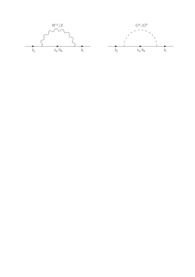
The Feynman diagrams of the self-energies which we need for the renormalization of the $Zb_{L}\bar{b}_{L}$ vertex are shown in Fig. 2. For the computation the programs FeynCalc[61] and FeynArts/FormCalc[62, 63] were used. The final result can be found in Appendix B. It is given in terms of general coupling factors so that it can be applied to other cases. The notation is similar to the one used in Ref. [22] so that the results can easily be compared. The results obtained for the vertex diagrams in Fig. 1 agree with those of Ref. [22]. The differences with respect to Ref. [22] arise from the renormalization of the mixing matrix, which we performed and which was not necessary in Ref. [22] as the authors did not take into account the case of a bottom quark mixing with heavy fermion partners. In our case, a finite result for $\delta g_{b_{L}}$ can only be obtained if the renormalization of the mixing matrix is included.

A comment is in order about contributions from the UV dynamics of the theory to the EWPTs. In Ref. [55] it was shown that there can be possibly large contributions to the $S$ parameter and the $Zb_{L}\bar{b}_{L}$ coupling from a non-decoupling of UV-physics. This can even give rise to logarithmically divergent contributions, as e.g. in the $Zb_{L}\bar{b}_{L}$ coupling due to an effective 4-fermion operator. The coupling constant of this operator is not relevant for the rest of our analysis and we therefore assume it to be small. There could be further finite contributions from the UV dynamics of the theory [55], which we neglect, however, since there is no reasonable way to estimate them in terms of the fields entering our effective Lagrangian.

3.4 The $\chi^{2}$ test and numerical results

The agreement of our model with the experimental data can be assessed by performing a $\chi^{2}$ test. The experimental values for the $\epsilon$ parameters and their correlation $\rho$ come from the LEP measurement at the $Z$ pole mass, see Ref. [64]. We use, however, the updated values of Ref. [45], which take into account a newer value of the $W$ mass [65]:

$$\begin{array}[]{lcl}\epsilon_{1}^{exp}&=&\left(5.4\pm 1.0\right)\cdot 10^{-3},\\ \epsilon_{2}^{exp}&=&\left(-7.9\pm 0.90\right)\cdot 10^{-3},\\ \epsilon_{3}^{exp}&=&\left(5.34\pm 0.94\right)\cdot 10^{-3},\\ \epsilon_{b}^{exp}&=&\left(-5.0\pm 1.6\right)\cdot 10^{-3},\\ \end{array}\hskip 28.45274pt\rho=\left(\begin{array}[]{cccc}1&0.80&0.86&0.00\\ 0.80&1&0.53&-0.01\\ 0.86&0.53&1&0.02\\ 0.00&-0.01&0.02&1\end{array}\right)\;.$$ (46)

The theory contributions to the parameters $\epsilon_{1},\epsilon_{2},\epsilon_{3}$ and $\epsilon_{b}$ are given by [16, 45],

$$\epsilon_{1}^{th} = (5.66-0.86\log(m_{h}/m_{Z}))\cdot 10^{-3}+\Delta\epsilon_{1}^{IR}+\alpha\Delta T\;,$$

$$\epsilon_{2}^{th} = (-7.11+0.16\log(m_{h}/m_{Z}))\cdot 10^{-3}\;,$$

$$\epsilon_{3}^{th} = (5.25+0.54\log(m_{h}/m_{Z}))\cdot 10^{-3}+\Delta\epsilon_{3}^{IR}+\Delta\epsilon_{3}^{UV}\;,$$

$$\epsilon_{b}^{th} = -6.48\cdot 10^{-3}+\delta g_{b_{L}}\;.$$ (47)

The first summands, respectively, are the SM corrections. The contributions $\Delta\epsilon_{i}^{UV/IR}$ and $\delta g_{b_{L}}$ have been given in subsections 3.1 – 3.3, and $\Delta T$ is the contribution to the $T$ parameter stemming from loops of heavy fermions. The covariance matrix is defined by

$$C_{ij}=\Delta\epsilon_{i}^{exp}\rho_{ij}\Delta\epsilon_{j}^{exp}\;,$$ (48)

where $i,j$ runs over $1,2,3$ and $b$. The parameters $\lambda_{t}$ and $\lambda_{b}$ are fixed by the requirement to recover the measured values of the top and bottom quark masses, $\lambda_{q}$ has been traded for $\sin\phi_{L}$, cf. Eq. (24), and the scale $f$ is given by $f=\sqrt{\xi}\,v$, so that the relevant set of free parameters for our model is $\{\xi,M_{10},\sin\phi_{L},y,m_{\rho}\}$. The $\chi^{2}$ is hence defined as

$$\chi^{2}(\xi,M_{10},\sin\phi_{L},y,m_{\rho})=\sum_{i,j}\left(\epsilon^{th}_{i}-\epsilon^{exp}_{i}\right)C^{-1}_{ij}\left(\epsilon^{th}_{j}-\epsilon^{exp}_{j}\right)\;.$$ (49)

The electroweak precision data indicate a preference for a heavy vector resonance, so that we fix the parameter $m_{\rho}$ to its maximal value of $4\pi f$ required by perturbativity. We found that this leads for most of the parameter sets to minimal or close to minimal values of $\chi^{2}$. We are therefore left with four degrees of freedom $\{\xi,M_{10},\sin\phi_{L},y\}$. A specific point in the parameter space fulfills the electroweak precision tests at 99% C.L. if it satisfies the criterion

$$\chi^{2}(\xi,M_{10},\sin\phi_{L},y)-\chi_{min}^{2}\leq 13.28\;,$$ (50)

where $\chi_{min}^{2}$ is the minimum of $\chi^{2}$ with $\chi_{min}^{2}\approx 0.87$. This is smaller than the SM value $\chi^{2}\approx 4.71$ as expected for a model with additional parameters.

A further constraint on the model is imposed by the recent measurement of the single top cross section at CMS[66], providing a lower limit on the CKM matrix element of $\lvert V_{tb}\rvert>0.92$ at 95% C.L.. The constraint on $V_{tb}$ will be discussed in more detail in Section 5.

We performed a scan over the parameter space, setting the top and bottom quark masses to $m_{t}=173.2$ GeV and $m_{b}=4.2$ GeV, respectively, and the Higgs boson mass to $m_{h}=125$ GeV. For the vector bosons masses we used $m_{W}=80.385$ GeV and $m_{Z}=91.1876$ GeV. The model parameters have been varied in the range

$$0\leq\xi\leq 1\;,\hskip 28.45274pt0<\sin\phi_{L}\leq 1\;,\hskip 28.45274pt|y|<4\pi\;,\hskip 28.45274pt0\leq M_{10}\leq 10\text{ TeV}\;.$$ (51)

In addition we only retained points for which $|V_{tb}|>0.92$. The result of the scan is shown in Fig. 3 (left) in the $\xi$-$\sin\phi_{L}$ plane. As can be inferred from the plot, for non-vanishing left-handed compositeness of the top and bottom quark, values of $\xi$ close to 0.2 are still allowed at 68% C.L.. For intermediate values, $0.4\raisebox{-3.69899pt}{~{}\shortstack{$<$ \\ [-0.07cm] $\sim$}}~{}\sin\phi_{L}\raisebox{-3.69899pt}{~{}\shortstack{$<$ \\ [-0.07cm] $\sim$}}~{}0.5$, parameter points with $\xi$ as large as $\xi\sim 0.5$ pass the constraints. In case of mostly composite left-handed quarks, $\sin\phi_{L}\raisebox{-3.69899pt}{~{}\shortstack{$>$ \\ [-0.07cm] $\sim$}}~{}0.9$, the constraints are passed at 99% C.L. for $\xi$ values up to about 0.35. It is the positive fermionic contributions to the $T$ parameter which drive it back into the region compatible with EWPTs.

Figure 3: Parameters passing the $\chi^{2}$ test of electroweak precision observables, fulfilling in addition $|V_{tb}|>0.92$, for a scan over $\xi$, $\sin\phi_{L}$, $y$ and $M_{10}$. Dark blue: $68\%$ C.L. region, medium blue: $95\%$ C.L. region and light blue: $99\%$ C.L. region. Left: the $\xi$-$\sin\phi_{L}$ plane. Right: $\Delta\chi^{2}$ versus $\xi$.

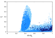
For $\sin\phi_{L}\raisebox{-3.69899pt}{~{}\shortstack{$<$ \\ [-0.07cm] $\sim$}}~{}0.25$, there are no allowed points, as for too low values of $\sin\phi_{L}$ the correct top mass cannot be obtained, cf. Eq. (27). The bottom quark being in the same doublet as the top quark, is hence mostly left-handed composite, as $\sin\phi_{Rb}$ must be small enough in order not to generate a too large bottom mass, cf. Eq. (27). Figure 3 (right) shows $\Delta\chi^{2}\equiv\chi^{2}-\chi^{2}_{min}$ versus $\xi$. The smallest values for $\Delta\chi^{2}$ are obtained for $0.01<\xi<0.2$. In contrast, high values of $\xi$ lead to large $\Delta\chi^{2}$, corresponding to a compatibility with the EWPT at 99% C.L.. Note that the SM limit is obtained for $\xi\to 0$ and $M_{10}\to\infty$. Due to the restriction of the scan to $M_{10}\leq 10$ TeV, it is not contained in the plot.

The impact of the bottom quark and its partners on the $\chi^{2}$ test is significant. Their inclusion not only requires the renormalization of the mixing matrix, which influences the finite terms. For some parameters in our scan the inclusion of the bottom partners in the loops can also change $\Delta\chi^{2}$ by a factor of 2. For the majority of the parameter points, however, the effect is much smaller. The contributions from diagrams with Higgs bosons in the loops alter $\Delta\chi^{2}$ by $\pm 2.9$% at most, for most parameter sets even less.

A comment is in order about the approximation of zero bottom quark mass in the computation of the corrections to the $Zb_{L}\bar{b}_{L}$ vertex. Neglecting the bottom mass changes the couplings of the bottom quark and of the bottom-like quarks to the vector bosons and Goldstone bosons. The effect, however, is small. The matrix element $X^{-1/3,L}_{bb}$, cf. Eq. (40), changes by maximally $1\%$ and the change in the corresponding matrix element for the Goldstone coupling is $\mathcal{O}(m_{b}/v)$. Compared to the largest matrix elements in the Goldstone coupling matrix this is less than a percent effect. We explicitly verified this numerically. Additional mass terms can arise in the loop corrections to the $Zb_{L}\bar{b}_{L}$ vertex. They are proportional to $m_{b}/m_{Z}$, and assuming that the couplings multiplying these terms are of the same order as the ones multiplying $m_{t}/m_{Z}$, they would only contribute to about 3% of the total matrix element. A conservative estimate of the error done by neglecting the bottom mass is therefore $5\%$, obtained by adding up linearly the error due to the kinematics and an estimate of $2\%$ for the error due to the change in the couplings.

As mentioned earlier loop contributions to the $T$ parameter from the top and bottom partners are important to render the model compatible with the EWPT for non-vanishing $\xi$ values. The implications of the electroweak precision data on the masses of the vector-like quarks can be inferred from Fig. 4. It shows $\Delta\chi^{2}$ as a function of $M_{10}$ which sets the scale for the top and bottom partner masses. As expected, the best compatibility of the model with the electroweak precision observables is obtained for non-vanishing masses of the order of 200 GeV$\raisebox{-3.69899pt}{~{}\shortstack{$<$ \\ [-0.07cm] $\sim$}}~{}M_{10}\raisebox{-3.69899pt}{~{}\shortstack{$<$ \\ [-0.07cm] $\sim$}}~{}$5 TeV. The bulk of the masses for the points which are best compatible with EWPT lies between about 800 GeV and 1.6 TeV, however. This is compatible with the lower limits from direct searches for heavy fermions, as will be discussed in detail in the next section.

Figure 4: $\Delta\chi^{2}$ versus $M_{10}$ of the parameters passing the $\chi^{2}$ test of electroweak precision observables, fulfilling in addition $|V_{tb}|>0.92$, for a scan over $\xi$, $\sin\phi_{L}$, $y$ and $M_{10}$. Dark blue: $68\%$ C.L. region, medium blue: $95\%$ C.L. region and light blue: $99\%$ C.L. region.

4 Constraints from Higgs Results and Direct Searches for Heavy Fermions

Further constraints on Composite Higgs Models come from the LHC Higgs search results. Both production processes and decay rates of the Higgs bosons are modified compared to the SM [35]. The modifications arising in our model shall be presented in the following. Subsequently, the constraints due to direct LHC searches for heavy fermions will be discussed.

4.1 Higgs Boson Production Processes

Gluon fusion: Gluon fusion [67] is the main Higgs production mechanism at the LHC and mediated already at leading order by loops of heavy quarks. In addition to the top and bottom quark loops present in the SM, in Composite Higgs Models also heavy quark partners contribute and the Higgs Yukawa couplings are modified. The QCD corrections to the process are important. In the SM they have been obtained at next-to-leading order (NLO) including the full quark mass dependence and in the heavy top mass limit [70]. They increase the cross section by 50-100%. At next-to-next-to-leading order (NNLO) QCD they are known in the heavy top quark limit [71], adding another 20%. Top quark mass effects on the NNLO cross section have been investigated in Ref. [72]. A resummation of soft gluons has been performed at next-to-next-to-leading log (NNLL) accuracy [73]. First results for the $\text{N}^{3}$LO QCD corrections have been given in Refs. [74]. For Composite Higgs Models the QCD corrections up to NNLO were calculated in Ref. [75], keeping the full bottom mass dependence through NLO. The two-loop Yukawa corrections to gluon fusion in the top partner singlet model have been presented in [76]. Note, that in Composite Higgs models without new heavy fermion partners the QCD corrected SM cross section can be taken over by adjusting the Higgs-Yukawa couplings. This cannot not be done, however, for the electroweak corrected process [77].

We implemented our model in the Fortran code HIGLU [78] in order to obtain the NLO QCD corrections with full mass dependence on the quark masses. This was done similar to the implementation of the 4th generation in HIGLU [79]. The Higgs Yukawa couplings had to be adjusted and all summations were extended to also include the loops with the new fermions. Electroweak corrections in Composite Higgs Models are not available and NNLO QCD corrections are only available in the heavy top quark limit, which cannot be applied for the bottom quark. We therefore only take into account the NLO QCD corrections. The $K$-factor obtained in this way,

$$K=\frac{\sigma_{NLO}}{\sigma_{LO}}\,,$$ (52)

is roughly the same as in the SM for NLO QCD corrections, up to deviations of less then $2\%$ depending on the specific parameter point, in agreement with Ref. [75].

In Ref. [43, 36, 44, 45] it was shown by applying the low-energy theorem [47] that the leading order gluon fusion cross section $\sigma$ with fermions in the fundamental representation and neglecting the mixing of the bottom quark with heavy partners, is given by the pure Higgs non-linearities,

$$\frac{\sigma}{\sigma_{SM}}\approx\frac{(1-2\xi)^{2}}{(1-\xi)}\;,$$ (53)

where $\sigma_{SM}$ denotes the SM gluon fusion cross section. The cross section, which only depends on $\xi$ but not on the details of the spectrum of the new fermions, is therefore always reduced compared to the SM for $\xi<0.75$. This result does not hold any more, however, if there exists a mixing with bottom partners [44, 46]. For the bottom quark the LET cannot be applied and the matrix element for the bottom-like contributions ${\cal M}_{bot}$ is given by

$$\mathcal{M}_{bot}\approx\mathcal{M}^{SM}_{LET}\left(\frac{1-2\xi}{\sqrt{1-\xi}}-\frac{y_{b}}{y_{SM}}\right)\;,$$ (54)

with ${\cal M}^{SM}_{LET}$ denoting the SM matrix element in the LET approximation, and $y_{b}$ and $y_{SM}$ being the bottom quark Yukawa coupling in our model and the SM, respectively. The gluon fusion cross section thus depends on the details of the spectrum through $y_{b}$. In Ref. [44] it was shown that this can even lead to an enhancement of the cross section for the gluon fusion process compared to the SM.

Vector boson fusion: Vector boson fusion [80] constitutes the next important Higgs production mechanism after gluon fusion. In the SM, the NLO QCD corrections to vector boson fusion are of $\mathcal{O}(10\%)$ of the total cross section [81, 82], the NNLO QCD corrections are at the percent level [83]. Electroweak corrections have been given in [84] and are of ${\cal O}(5\%)$.

In our model, the cross section at NLO QCD can be obtained from the SM cross section by multiplying it with a factor $(1-\xi)$ stemming from the modified Higgs couplings to massive vector bosons $V$ due to the Higgs non-linearities, cf. Eq. (10),

$$\sigma_{VBF}^{CHM}=(1-\xi)\sigma_{VBF}^{SM}\;.$$

The cross section is reduced compared to the SM cross section, which we calculated at NLO QCD with the Fortran code VV2H [85]. Again, neither electroweak (EW) corrections nor NNLO QCD corrections can be taken into account.

Higgs-strahlung: In Higgs-strahlung the Higgs boson is radiated off vector bosons. The NLO QCD corrections increase the cross-section by ${\cal O}(30\%)$ [82, 86], the NNLO QCD corrections are small [87]. The electroweak corrections for the SM decrease the cross section by $\mathcal{O}(5-10\%)$ [88]. We proceed analogously to vector boson fusion and only take into account NLO QCD corrections. The SM cross section at NLO QCD[82, 86] has been computed with the code V2HV[85] and subsequently multiplied with the appropriate modification factor to obtain the Composite Higgs production cross section,

$$\sigma_{Wh/Zh}^{CHM}=(1-\xi)\sigma_{Wh/Zh}^{SM}\;.$$ (55)

Associated production with top quarks: The cross section for associated production of a SM Higgs boson of $m_{h}=125$ GeV with a top quark pair [89] is two orders of magnitudes smaller than the gluon fusion cross section. We took the SM cross section including NLO QCD corrections [90] from the LHC cross section working group [91] and modified it to take into account the Higgs-top Yukawa coupling of our model,

$$\sigma^{CHM}(t\bar{t}h)=\left(\frac{g_{tth}}{g_{tth}^{SM}}\right)^{2}\sigma^{SM}(t\bar{t}h)\;.$$ (56)

The coupling $g_{tth}$ is obtained from the matrix Eq. (29) after rotation to the mass eigenstates.

4.2 Higgs Boson Decays

The Composite Higgs branching ratios have been calculated with the Fortran code HDECAY[92], which we have adapted to our model by proceeding as follows: To get the Composite Higgs fermionic decay widths, all corresponding SM widths have been modified as

$$\Gamma^{CHM}_{h\to f\bar{f}}=\begin{cases}\left(\frac{(U_{L}^{b\dagger}G_{hb\bar{b}}U_{R}^{b})_{b\bar{b}}}{g_{hb\bar{b}}^{SM}}\right)^{2}\Gamma^{SM}_{h\to f\bar{f}}\hskip 28.45274pt&\mbox{if }f=b\;,\\ \frac{(1-2\xi)^{2}}{1-\xi}\Gamma^{SM}_{h\to f\bar{f}}\hskip 28.45274pt&\mbox{if }f=c,s,\mu,\tau\;.\end{cases}$$ (57)

The decays into top quarks are not relevant for a 125 GeV Higgs boson. In the decay width into bottom quarks the factor $(U_{L}^{b\dagger}G_{hb\bar{b}}U_{R}^{b})_{b\bar{b}}$ denotes the matrix element relevant for the bottom quark coupling after rotation of the Higgs Yukawa coupling matrix $G_{hb\bar{b}}$, Eq. (30), into the basis of the mass eigenstates. The prefactor for the decays into the charm ($c$), strange ($s$), muon ($\mu$) and $\tau$ final states, which are elementary particles in contrast to the top and bottom quark, is due to the Higgs non-linearities, implying a Yukawa coupling

$$g_{hf\bar{f}}^{CHM}=\frac{1-2\xi}{\sqrt{1-\xi}}\,g_{hf\bar{f}}^{SM}$$ (58)

for the fermions in the fundamental and antisymmetric representation [7]. The decays into vector bosons $V$ are obtained from the corresponding SM widths by

$$\Gamma^{CHM}_{h\to VV}=(1-\xi)\,\Gamma^{SM}_{h\to VV}\;.$$ (59)

For the loop-induced decays also the top and bottom partners have to be taken into account. The decay widths $h\to\gamma\gamma$ and $h\to gg$ (at leading order) are modified as

$$\Gamma_{\gamma\gamma}=\frac{G_{F}\alpha^{2}m_{h}^{3}}{128\sqrt{2}\pi^{3}} \left|\,\sum_{i=1}^{5}\frac{16}{9}\frac{v(U_{L}^{t\dagger}G_{htt}U_{R}^{t})_{ii}}{m_{t_{i}}}\,A_{1/2}(\tau_{t_{i}})+\sum_{i=1}^{4}\frac{4}{9}\frac{v(U_{L}^{b\dagger}G_{hbb}U_{R}^{b})_{ii}}{m_{b_{i}}}\,A_{1/2}(\tau_{b_{i}})\right.$$ (60)

$$\left.\,+\frac{4}{3}\frac{1-2\xi}{\sqrt{1-\xi}}\,A_{1/2}(\tau_{\tau})+\frac{16}{9}\frac{1-2\xi}{\sqrt{1-\xi}}\,A_{1/2}(\tau_{c})+\sqrt{1-\xi}A_{1}(\tau_{W})\right|^{2}\;,$$

$$\Gamma_{gg}=\frac{G_{F}\alpha_{s}^{2}m_{h}^{3}}{36\sqrt{2}\pi^{3}} \left|\,\sum_{i=1}^{5}\frac{v(U_{L}^{t\dagger}G_{htt}U_{R}^{t})_{ii}}{m_{t_{i}}}A_{1/2}(\tau_{t_{i}})+\sum_{i=1}^{4}\frac{v(U_{L}^{b\dagger}G_{hbb}U_{R}^{b})_{ii}}{m_{b_{i}}}A_{1/2}(\tau_{b_{i}})\right.$$ (61)

$$\left.\,+\frac{1-2\xi}{\sqrt{1-\xi}}A_{1/2}(\tau_{c})\right|^{2}\;,$$

where we introduced the notation

$$\tau_{W}=\frac{4M_{W}^{2}}{m_{h}^{2}},\hskip 14.22636pt\tau_{t_{i}/b_{i}}=\frac{4m_{t_{i}/b_{i}}^{2}}{m_{h}^{2}},\hskip 14.22636pt\tau_{c}=\frac{4m_{c}^{2}}{m_{h}^{2}}\hskip 14.22636pt\text{and}\hskip 14.22636pt\tau_{\tau}=\frac{4m_{\tau}^{2}}{m_{h}^{2}}\;.$$ (62)

The masses of the top quark and its four heavy partners are denoted by $m_{t_{i}}$ ($i=1,...,5$), the masses of the bottom quark and its three heavy partners by $m_{b_{i}}$ ($i=1,...,4$), $m_{c}$ is the charm quark mass and $m_{\tau}$ the mass of the $\tau$-lepton. The loop functions are given by

$$A_{1}(\tau)=-[2+3\tau+3\tau(2-\tau)f(\tau)]$$ (63)

for $W$ bosons in the loop, and

$$A_{1/2}(\tau)=\frac{3}{2}\tau[1+(1-\tau)f(\tau)]\;,$$ (64)

for fermions in the loop, with

$$f(\tau) =\begin{cases}\arcsin^{2}\frac{1}{\sqrt{\tau}}&\text{for }\,\tau\geq 1\;,\\ -\frac{1}{4}\left[\log(\frac{1+\sqrt{1-\tau}}{1-\sqrt{1-\tau}})-i\pi\right]^{2}&\text{for }\,\tau<1\;.\end{cases}$$ (65)

Remark that in the LET the contribution due to the loops of the top quark and its partners reduces to the pure Higgs non-linearities which means that it is simply given by the SM top loop contribution modified with the coupling factor $(1-2\xi)/\sqrt{1-\xi}$, parallel to the charm and $\tau$ loop contributions. For the bottom loops, where the LET cannot be applied, this is not the case.

We do not give an explicit formula for the decay $h\to Z\gamma$ as we will not investigate this channel any further, which due to its smallness practically does not affect the total decay width. All decays are taken at NLO QCD if available in HDECAY, see [93, 94] for details of the implementation. Neither electroweak corrections nor NNLO QCD corrections were taken into account. For slight deviations from the SM, EW corrections can be included as described in Ref. [93]. We will nevertheless neglect them as we also want to deal with possibly large values of $\xi$.

4.3 Constraints from Searches for Heavy Fermions and from Flavour Physics

The strongest bounds from direct searches for new vector-like fermions come from ATLAS [96, 97] and CMS [98, 99]. Recently, both collaboration have provided direct bounds on the mass of the new fermions as a function of their branching ratios into SM particles [96, 97, 98, 99], since the fermion pair production is a pure QCD process, which only depends on the mass of the particle, and can be computed independently of the model. The new top-like quarks can decay into $Wb$, $ht$ or $Zt$, the new bottom-like fermions into $Wt$, $Zb$ or $hb$ and the new charge-5/3 fermions into $Wt$. We have calculated the decay widths in our model using the formulae of Ref. [45] (see also Ref. [13]), and directly compared them with the bounds quoted by the collaborations. The bounds are obviously valid for the lightest of the composite fermions, but not necessarily for the heavier ones. The reason is that a composite fermion, which is massive enough to decay into a lighter composite fermion and a $W$ or $Z$ boson, could have a substantial decay width into the corresponding channel, hence its branching ratios into the SM particles would be reduced.

In the specific model studied in this work, the situation is made quite simple since the lightest of all composite fermions is always a fermion of charge 5/3, decaying therefore 100% into $Wt$. The strongest bound on charge-5/3 fermions comes from the CMS analysis [100],

$$m_{\chi}\geq 770~{}\textrm{GeV}.$$ (66)

The bound on the bottom-like quarks turns out to be less stringent than for the charge-5/3 fermions, but for top-like quarks ATLAS has limits extending up to around 850 GeV in the case of a decay mostly in $ht$ [96]. This limit can be applied as it is to the lightest of the charge-2/3 fermions, since it is in any case below the threshold for the decay of a heavy top-like partner into $\chi W$ due to the bound of Eq. (66). In our model, however, the search for top-like fermions is never more constraining than the search for the charge-5/3 ones. In the future, and mostly with the LHC operating at 14 TeV, important bounds will be derived from single production of a heavy vector-like fermion, see e.g. [101, 14], but such bounds are not yet available.

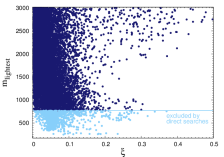
In Fig. 5 we show the mass of the lightest composite fermion as a function of $\xi$. The points in the plot are the ones which pass the EWPT at 99% C.L. and fulfill $|V_{tb}|>0.92$. The light blue points are excluded by direct searches at 95% C.L., the dark blue points are not excluded. The line in the plot marks the exclusion limit from CMS of 770 GeV on charge-5/3 fermions. As can be inferred from the plot this exclusion limit eliminates quite some parameter space for $\text{m}_{\text{lightest}}>770$ GeV. No points are excluded above masses of the lightest partner of 770 GeV which confirms that the bounds on heavy top partners of up to 850 GeV for large branching ratios of $T\to hb$ do not lead to any additional constraints.

Flavour physics can lead to further constraints on Composite Higgs Models. They depend, however, on the exact flavour structure of the model. Anarchic flavour structures seem to be strongly constrained by CP violating observables in the Kaon system[24]. Implementing minimal flavour violation can, however, avoid these constraints [27]. In this case, also the light quarks are required to be composite, which can significantly change the Higgs phenomenology [46]. While dijet searches put constraints on the up and down quarks [102], the second generation quarks are practically not constrained [30]. Alternatively, the top quark can be treated differently than the light quarks [28]. The flavour bounds can still be satisfied, and the constraints from EWPT and searches for compositeness are relaxed, as the first two generations are mostly elementary. Both the left-handed and right-handed top can be composite in this case. Bounds on the masses of the lightest fermionic resonance have been obtained in Ref. [31] and depend on the specific flavour symmetry. We do not assume a specific flavour model and therefore do not further discuss constraints from flavour physics. For additional discussions of flavour constraints on Composite Higgs Models, see e.g. Ref. [29].

Figure 5: Spectrum of the lightest composite fermion as function of $\xi$. The points in the plot are obtained from a scan over $\xi,\,y,\,M_{10}$ and $\sin\phi_{L}$ and fulfill the EWPT at 99% C.L. and $|V_{tb}|>0.92$. The light blue points are excluded by direct searches for vector-like fermions at 95% C.L., the dark blue points are not excluded.

5 Numerical results

In this section, we show numerical results for a combined analysis taking into account the constraints from electroweak precision observables, Higgs search results, the measurement of $V_{tb}$ and the direct searches for heavy fermions. We make a random scan over the parameter ranges defined in Eq. (51) and with the SM input values as given in section 3.4. In order to test the agreement of our model with the aforementioned constraints we perform a global $\chi^{2}$ test similar to that of Refs. [103],

$$\chi^{2}=\chi^{2}_{EWPT}+\chi^{2}_{Higgs}+\chi^{2}_{V_{tb}}\;.$$ (67)

Notice that the constraints from direct searches of new heavy fermions are not included in the global $\chi^{2}$ test, but rather imposed directly by only taking into account points which are not excluded at $95\%$ C.L. by direct searches. The $\chi^{2}_{EWPT}$ is the $\chi^{2}$ for the electroweak precision tests defined in Eq. (49).

Regarding the constraints from the Higgs boson, the ATLAS and CMS collaborations provide the signal strengths

$$\mu(X)=\frac{\sigma(pp\to h)\cdot BR(h\to X)}{\sigma(pp\to h)_{SM}\cdot BR(h\to X)_{SM}}$$ (68)

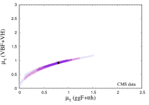
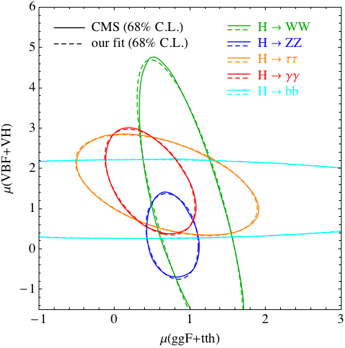
including the correlations between the combination of the vector boson fusion (VBF) and the Higgs-strahlung (VH) production modes (VBF+VH) and the combination of gluon fusion (ggF) and the associated production with a top quark pair (tth) (ggF+tth) [104, 105]. The results have been given as likelihood contours, which correspond approximately for each Higgs boson decay channel to the ellipses obtained from a $\chi^{2}$ test with two variables. We can therefore write

$$\chi^{2}_{Higgs}=\sum_{\scriptscriptstyle channels}\sum_{\scriptscriptstyle i,j=1,2}(\mu_{i}^{exp}-\mu_{i}^{th})C_{ij}^{-1}(\mu_{j}^{exp}-\mu_{j}^{th})\;,$$ (69)

where the best-fit points from the experiments are denoted by $\mu^{exp}_{1}=\mu^{exp}_{\scriptscriptstyle ggF+tth}$ and $\mu^{exp}_{2}=\mu^{exp}_{\scriptscriptstyle VBF+VH}$ and the covariance matrix $C$ is defined as

$$C=\left(\begin{array}[]{c c}\Delta\mu_{\scriptscriptstyle ggF+tth}^{2}&\rho\Delta\mu_{\scriptscriptstyle ggF+tth}\,\Delta\mu_{\scriptscriptstyle VBF+VH}\\ \rho\Delta\mu_{\scriptscriptstyle ggF+tth}\,\Delta\mu_{\scriptscriptstyle VBF+VH}&\Delta\mu_{\scriptscriptstyle VBF+VH}^{2}\end{array}\right),\hskip 14.22636pt\Delta\mu_{i}\equiv\sqrt{\left(\Delta\mu_{i}^{exp}\right)^{2}+\left(\Delta\mu_{i}^{th}\right)^{2}}\;.$$ (70)

The values of $\mu^{exp}_{i}$, $\Delta\mu^{exp}_{i}$ and $\rho$ are extracted from the experimental results, see Appendix C. The theoretical value $\mu^{th}_{1}=\mu^{th}_{\scriptscriptstyle ggF+tth}$ ($\mu^{th}_{2}=\mu^{th}_{\scriptscriptstyle VBF+VH}$) in the final state channel $X$ is obtained by computing in our model the sum of the ggF and tth (VBF and VH) production cross sections and multiplying this with the branching ratio into the final state $X$. Subsequently, the value obtained is normalized to the corresponding SM rate. The final states that we take into account are $X=W,Z,\gamma,b$ and $\tau$. The theoretical uncertainties $\Delta\mu_{i}^{th}$ stem from the scale and PDF uncertainties of the total cross section. We use the relative theoretical uncertainties of the SM throughout the numerical analysis, as we checked explicitly for some parameter points that the theoretical uncertainties obtained within our model are only slightly modified compared to the SM. This leads then to $\Delta\mu_{\scriptscriptstyle VBF+VH}^{th}=0$ and very small $\Delta\mu_{\scriptscriptstyle ggF+tth}^{th}$. As we computed all the production cross sections at NLO QCD, the uncertainties are the ones given at this order. Note also that for the $b\bar{b}$ channel, there is no information available from ATLAS on the correlation. In this case, we then defined

$$\chi^{2}_{h\to b\bar{b}}=\frac{(\mu^{exp}_{b}-\mu^{th}_{b})^{2}}{(\Delta\mu^{exp}_{b})^{2}+(\Delta\mu^{th}_{b})^{2}}\;,$$ (71)

where $\mu_{b}$ is obtained from the sum of all VBF, VH, ggF and tth production modes times the branching ratio into $b\bar{b}$ normalized to the corresponding SM rate.

The constraint from the measured value of the CKM matrix element $|V_{tb}|$ can be treated in two different ways. Either all points with $|V_{tb}|>0.92$ are rejected, or the best fit value quoted by the experiments is included in the $\chi^{2}$ test. The CMS collaboration measured the value to be [66]

$$|V_{tb}^{exp}|=1.02\pm 0.046\;.$$ (72)

The value of $|V_{tb}^{th}|$ in the model considered in this work is taken from the $W$ coupling to the top and the bottom quark. For the SM we assume $|V_{tb}^{th}|=1$. The couplings of all other SM quarks to the $W$ boson in our model are the same as in the SM. A $\chi^{2}$ test for the constraint on $V_{tb}$ can therefore be written as

$$\chi^{2}_{V_{tb}}=\frac{(|V_{tb}^{exp}|-|V_{tb}^{th}|)^{2}}{(\Delta V_{tb}^{exp})^{2}}\;.$$ (73)

	$|V_{tb}|>0.92$			$|V_{tb}|$ in $\chi^{2}$
Experiment	$\xi$	$\chi^{2}/n$	$\chi^{2}_{n}$	$\xi$	$\chi^{2}/n$	$\chi^{2}_{n}$
ATLAS	0.105	8.06/9	0.90	0.096	12.34/10	1.23
	0.0	17.54/13	1.35	0.0	17.73/14	1.25
CMS	0.057	5.22/10	0.52	0.055	6.36/11	0.58
	0.0	9.90/14	0.71	0.0	10.09/15	0.67

Table 2: Global $\chi^{2}$ results for the best fit point taking into account EWPT and the Higgs results for ATLAS and CMS, respectively: Left: For parameter points which fulfill $|V_{tb}|>0.92$. Right: When including the measured value of $|V_{tb}|$ in the $\chi^{2}$ test. The lines for $\xi=0.0$ list for comparison the SM values. The number of degrees of freedom $n$ are counted naively as the difference between the number of observables and the number of parameters in the model, and $\chi^{2}_{n}\equiv\chi^{2}/n$.

We report in Table 2 the $\chi^{2}$ values of the best fit points for our model and, for comparison, the ones for the SM. They are given for the two different ways of including the constraint from $V_{tb}$. The best fit point can be different in both cases. The global $\chi^{2}$ is obviously increased when including $V_{tb}$, although in the SM limit where $|V_{tb}^{th}|=1$ was used, the change is small. The constraint from $|V_{tb}|$ mainly affects scenarios with lower masses of the lightest resonance. We distinguish between the data for the Higgs rates of the two experiments ATLAS [104] and CMS [105], as no combination exists so far. The CMS data turns out to be better described than the ATLAS data. The best fit points are obtained for values of $\xi\approx 0.1$ for ATLAS and for $\xi\approx 0.05$ for CMS. In our Composite Higgs Model their $\chi^{2}$ is slightly smaller than in the SM, due to the larger number of free parameters. The value of $\chi^{2}_{n}\equiv\chi^{2}/n$ gives an estimate of the relative goodness of the fit. Note, however, that the counting of the number of degrees of freedom is not obvious as the SM limit is reached when $\xi\to 0$ and $M_{10}\to\infty$, and then the other parameters become meaningless.

Figure 6: $\Delta\chi^{2}=\chi^{2}-\chi_{min}^{2}$ taking into account the Higgs results of ATLAS (left) and CMS (right), as a function of $\xi$. The dark blue points do better than the SM, the light blue points have a higher $\Delta\chi^{2}$.

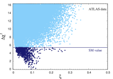
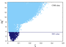
Figure 6 shows, as a function of $\xi$, $\Delta\chi^{2}=\chi^{2}-\chi_{min}^{2}$, where $\chi^{2}$ is defined in Eq. (67) and $\chi^{2}_{min}$ is the value of the best fit point. The color distinguishes between points which do better than the SM and those doing worse. For the CMS results only points with $\xi\lesssim 0.1$ have a lower $\Delta\chi^{2}$ than the SM, while for the ATLAS results this is the case for points up to $\xi\lesssim 0.25$, although most of the scenarios doing better than the SM are for $\xi\raisebox{-3.69899pt}{~{}\shortstack{$<$ \\ [-0.07cm] $\sim$}}~{}0.15$. Figure 7 shows $\Delta\chi^{2}$ as a function of the top and bottom partner mass scale $M_{10}$ for the ATLAS data (left) and the CMS data (right). The lower limit on $M_{10}$ is due to the inclusion of the direct search bounds on heavy fermion masses. The bulk of the masses leading to scenarios doing better than the SM lies around 1–2 TeV. This is mainly due to the EWPT. For very heavy fermion masses the compatibility with the data is not as good.

Figure 7: $\Delta\chi^{2}=\chi^{2}-\chi_{min}^{2}$ taking into account the Higgs results of ATLAS (left) and CMS (right), as a function of $M_{10}$. The dark blue points do better than the SM, the light blue points have a higher $\Delta\chi^{2}$.

Figure 8: Fit results obtained from a scan over $\xi$, $y$, $\sin\phi_{L}$ and $M_{10}$ taking into account the EW precision data, the measured value of $|V_{tb}|$ and the ATLAS Higgs results, shown in the $\mu_{\scriptscriptstyle ggF+tth}-\mu_{\scriptscriptstyle VBF+VH}$ plane for the channels $\gamma\gamma$ (top left), $W^{+}W^{-}$, $ZZ$ (both top right) and $\tau^{+}\tau^{-}$ (bottom). The black rhombus in the plot is the best fit point. The color code in the plots indicates from dark to light colors the $1\sigma$, $2\sigma$, $3\sigma$ and $5\sigma$ regions obtained from the $\chi^{2}$ test with four degrees of freedom.

In Fig. 8, we show the fit results of our parameter scan in the $\mu_{\scriptscriptstyle ggF+tth}-\mu_{\scriptscriptstyle VBF+VH}$ plane for the Higgs decay channels into $\gamma,W,Z$ and $\tau$ pairs, respectively. The color code indicates from dark to light colours the $1\sigma$, $2\sigma$, $3\sigma$ and $5\sigma$ regions obtained from the $\chi^{2}$ test as defined in Eq. (67) with the experimental Higgs results reported by ATLAS. The black rhombus in the plot marks the best fit point which corresponds to the minimum value obtained from the $\chi^{2}$ test. The fit contours for $W$ and $Z$ bosons are the same as their couplings are modified in the same way due to the custodial symmetry of the model and they are therefore depicted in the same plot. As can be inferred from Fig. 8 (top left), the ATLAS data prefer an enhanced Higgs to $\gamma\gamma$ rate. Also the rate into vector bosons is somewhat enhanced whereas the best fit point in the $\tau$ channel shows a nearly SM like rate. 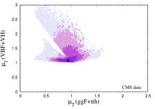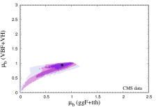The same plots for the CMS Higgs results can be found in Fig. 9, except that additionally the $b\bar{b}$ channel is shown (bottom left), as CMS provides information about the (VBF+VH) and (ggF+tth) production modes and their correlation in the $b\bar{b}$ channel. The best fit points are near the SM-like rates in the $\gamma\gamma$ final state, while the rates in the $W^{+}W^{-}$, $ZZ$, $b\bar{b}$ and $\tau^{+}\tau^{-}$ channel are slightly reduced in the (ggF+tth) production mode with respect to the SM value. From Fig. 8, bottom, and Fig. 9, bottom right, respectively, we see that in the $\tau\tau$ final state the region of the points passing the test is very narrow. In fact this behaviour is already found before applying the EWPT and $|V_{tb}|$ constraints, i.e. the rates for both production channel combinations behave very similarly. The reason is that the behaviour of $BR(h\to\tau\tau)$ and of the production in (ggF+tth) is correlated, and hence the rate $\mu_{\tau}(VBF+VH)$ is correlated with the rate $\mu_{\tau}(ggF+tth)$ via the decay channel. The former can be easily understood if for the moment the heavy fermion contributions are left aside (assuming simply the fermion partners to be very heavy) and the pure Higgs non-linearities are taken into account. Then both (ggF+tth) production and the decay into $\tau\tau$ go to zero for $\xi=0.5$ as all the Higgs-Yukawa couplings are proportional to $(1-2\xi)/\sqrt{1-\xi}$ in this case. With decreasing $\xi$ from 0.5 to 0 then both the (ggF+tth) production cross section and the branching ratio (cf. Fig. 2 in [35]) increase. And also the (VBF+VH) production cross section, which is proportional to $(1-\xi)$, increases. Due to this strong correlation between the rates from the two production channel combinations there remains only a small strip in the $\mu_{\tau}(ggF+tth)-\mu_{\tau}(VBF+VH)$ plane. The effect of imposing the constraints from EWPT and $|V_{tb}|$ is then to simply divide this strip into 1$\sigma$ to 5$\sigma$ regions. The region in the $b$-quark final state, cf. Fig. 9 (bottom left), is explained similarly. It is somewhat more spread because the Higgs coupling to the bottom quarks and hence the branching ratio in the $b\bar{b}$ final state is influenced by the compositeness of the bottom quark. For the $WW$, $ZZ$ and $\gamma\gamma$ final states there is no such strong correlation between the rates, as the rates from (VBF+VH) production do not vanish for $\xi=0.5$ in this case.

Figure 9: Fit results obtained from a scan over $\xi$, $y$, $\sin\phi_{L}$ and $M_{10}$ taking into account the EW precision data, the measured value of $|V_{tb}|$ and the CMS Higgs results, shown in the $\mu_{\scriptscriptstyle ggF+tth}-\mu_{\scriptscriptstyle VBF+VH}$ plane for the channels $\gamma\gamma$ (top left), $W^{+}W^{-}$, $ZZ$ (both top right), $b\bar{b}$ (bottom left) and $\tau^{+}\tau^{-}$ (bottom right). The black rhombus in the plot is the best fit point. The color code in the plots indicates from dark to light colors the $1\sigma$, $2\sigma$, $3\sigma$ and $5\sigma$ regions obtained from the $\chi^{2}$ test with four degrees of freedom.

So far we have not taken into account the constraint on the mass of the lightest top partner, as given in Refs. [8, 9, 10]. These works assumed that the Higgs potential is dominated by the first resonances in the composite sector, and the lightness of the Higgs boson is related to the lightness of the top partners. An approximate bound on the mass $m_{Q}$ of the lightest top partner was given in Ref. [10] based on sum rules:

$$m_{Q}\lesssim\frac{m_{h}\pi v}{m_{t}\sqrt{N_{c}}\sqrt{\xi}}\;,$$ (74)

where $N_{c}=3$ is the number of colors. This bound eliminates automatically large values of $\xi$, as too low masses for the lightest top partner are already excluded by direct searches. Requiring the lightest top partner to satisfy Eq. (74), the best fit points are modified compared to Table 2 and the quality of the fit becomes slightly worse. The new best fit values for $\xi$ and $\chi^{2}$, taking into account this bound, can be found in Table 3. The $\xi$ value for the ATLAS results becomes somewhat smaller, whereas for the CMS results it hardly changes. Note, however, that the bound Eq. (74) can be relaxed if QCD corrections from a new heavy gluon of the strong sector are included [11]. The details depend of course on the mass of the heavy gluon and its couplings.

Experiment	$\xi$	$m_{t_{lightest}}$	$\chi^{2}$
ATLAS	0.067	806 GeV	13.71
CMS	0.055	1335 GeV	7.17

Table 3: Global $\chi^{2}$ results for the best fit point respecting EWPT, $|V_{tb}|$ and the Higgs search results by ATLAS and CMS, respectively, with the corresponding $\xi$ value and the mass of the lightest top partner $m_{t_{lightest}}$. In addition the constraint of Eq. (74) originating from the connection between a light Higgs boson and light resonances has been taken into account.

So far we have not discussed the question of fine-tuning in our model. Experimental data require the electroweak scale $v$ to be significantly smaller than the strong symmetry breaking scale $f$. This is possible through cancellations in the Higgs potential with a precision that is given by $\Delta=f^{2}/v^{2}$. The exact tuning, however, crucially depends on the actual structure of the Higgs potential, which in turn is controlled by the choice of the fermion representations [8, 9, 10]. Therefore $f^{2}/v^{2}=1/\xi$ can only be regarded as a measure for the minimal tuning, while the detailed investigation of the amount of fine-tuning of the model would require the calculation of the Higgs potential. This is beyond the scope of the paper. We therefore restrict ourselves to state that best compatibility of our investigated model with all constraints, that have been taken into account, is achieved for $\xi$ values around 0.05 which corresponds to a minimal tuning of $\Delta=20$. Note that we also found scenarios with lower $\chi^{2}$ than in the SM for values of $\xi\sim 0.3$ which would imply lower tuning. Furthermore, in composite Higgs models a light Higgs mass can in general only be achieved with moderate tuning if the mass of the lightest top partner is not too heavy [8, 9, 10]. With masses for the lightest top partner of the order of 1 TeV our model can therefore be estimated to be moderately tuned.

6 Conclusions

Composite Higgs Models allow for a smooth deviation from the SM with identical particle content at low energy. A light narrow Higgs boson arises as pseudo-Nambu Goldstone boson from the spontaneous breaking of a strong sector and is separated by a mass gap from the other resonances of the strong sector. Heavy fermions acquire their masses by applying the idea of partial compositeness: The quark masses are generated through the mixing with the strong sector by coupling the SM quarks linearly with the heavy partners of the strong sector. This is in particular interesting for heavy quarks like the top quark. While in previous investigations the bottom quark mass has been introduced ad hoc into the model, we applied in this work the mass generation through partial compositeness also to the bottom sector. The model is challenged by strong constraints from the measurement of the $Zb_{L}\bar{b}_{L}$ coupling. The latter is safe from large corrections only if the $b_{L}$ belongs to a bi-doublet of $SU(2)_{L}\times SU(2)_{R}$. Starting from a global symmetry group $SO(5)$, the minimal representation which fulfills this requirement and incorporates partial compositeness for the bottom quark is the antisymmetric ${\bf 10}$. Based on a model with the coset $SO(5)/SO(4)$ and the top and bottom quarks embedded into this representation, we investigated the phenomenology of Composite Higgs Models with both top and bottom quarks being partially composite objects.

We addressed the constraints due to electroweak precision measurements. In particular we calculated the loop corrections to the $Zb_{L}\bar{b}_{L}$ coupling due to the heavy top and bottom partner contributions. The latter did not existed in the literature before and required the renormalization of the mixing matrix. Subsequently, we performed a $\chi^{2}$ test taking into account EWPT and the recent measurement of $|V_{tb}|$. It turned out that the fermionic loop contributions drive back the $T$ parameter into the region compatible with EW precision data, so that the Composite Higgs Model for some parameter combinations even does better than the SM, which is not too astonishing in view of the enlarged set of parameters. The additional contributions from the bottom partners turned out to have a significant impact on the $\chi^{2}$ test so that $\xi$ values of up to 0.2 (0.4) can be obtained at 68% (99%) confidence level, corresponding to a compositeness scale $f$ of 550 GeV (390 GeV).

We then proceeded to test the model with respect to its compatibility with the LHC searches for new heavy fermions and with the LHC Higgs search results. For the latter we computed the production cross sections and branching ratios taking into account the modified Higgs couplings to the SM particles and the new heavy fermion contributions in the loop induced processes such as gluon fusion and the decay into photons.

It has been shown before, by applying the low-energy theorem, that if the determinant of the heavy top mass matrix factorizes into a part depending on the Higgs non-linearities and a part depending on the details of the heavy spectrum – as it is the case here and in most minimal models – then the loop-induced Higgs coupling to gluons that enters the dominant gluon fusion Higgs production process at the LHC is not sensitive to the details of the spectrum of the top sector, but only depends on the Higgs non-linearities. In the case of bottom loops, however, the LET cannot be applied any more, so that the gluon fusion production cross section now shows a dependence on the masses of the heavy bottom partners. We performed a global $\chi^{2}$ test based on the Higgs signal strengths provided by ATLAS and CMS, on the EWPT and on the measurement of $|V_{tb}|$. Keeping in addition only those parameter points which fulfill the limits from the searches for heavy fermions, we found that numerous scenarios are compatible with all the constraints, with the best fit point being closer to the SM when considering the CMS data than for the ATLAS data. For CMS data the best fit point is at $\xi\sim 0.05$, for ATLAS data at $\xi\sim 0.1$. Seeking for a natural explanation of the light Higgs boson mass the lightest top partner cannot be too heavy. Taking this into account the global $\chi^{2}$ for the best fit point deteriorates and is now obtained for $\xi\sim 0.07$ for the ATLAS data, while it hardly changes for the CMS data. The corresponding lightest top mass here is about 1.3 TeV, for ATLAS data it is around 800 GeV.

In summary, being guidelined by the principle of introducing a minimum amount of new parameters, we investigated a Composite Higgs Model with composite top and bottom quarks. We found that the model is in very good agreement with the EWPT, the measurement of $V_{tb}$ and the LHC data from the Higgs and heavy fermion searches. Composite bottom partners can even ameliorate the compatibility of the model with the EWPT. Though the characteristic scale of the strong sector is pushed to somewhat higher values when applying in addition the connection between a light Higgs mass and the lightest new resonance of the model, it is still in good agreement with all the constraints.

Acknowledgments

We would like to thank the ATLAS Exotics Group and in particular Mark Cooke and Merlin Davies for giving us access to the results of ATLAS searches for top partners. We also want to thank A. Azatov, A. Belyaev, R. Contino, L. Di Luzio, M. Serone, M. Spira and M. Wiebusch for helpful discussions, and C. Grojean for reading the draft. R.G. and M.M. are supported by the DFG/SFB-TR9 Computational Particle Physics. R.G. acknowledges financial support by the Landesgraduiertenförderung des Landes Baden-Württembergs. The CP³-Origins centre is partially funded by the Danish National Research Foundation, grant number DNRF90.

Appendix

Appendix A The Fermion Couplings to the Gauge Bosons and to the Goldstone bosons

For the calculation of the New Physics contributions of our model to the $Zb_{L}\bar{b}_{L}$ coupling we need the couplings of the fermions to the gauge bosons and to the Goldstone bosons. The former are obtained from Eq. (14) after rotation to the mass eigenstates. The fermion-Goldstone boson couplings have been derived from the Lagrangian given in Eq. (13), by using Eq. (5) and making the identifications according to Eq. (31). In order to define the couplings in a general way, the Lagrangians for the specific couplings of the $W$ bosons, the $Z$ bosons, the charged Goldstone bosons $G^{\pm}$ and the neutral Goldstone boson $G^{0}$ to the quarks $\Psi$ of charge $Q$, respectively, $Q-1,$ are parameterized as follows

$$\mathcal{L}_{W} =\frac{g}{\sqrt{2}}W_{\mu}^{+}\bar{\Psi}_{Q}^{i}\gamma^{\mu}\left(V_{ij}^{QL}P_{L}+V_{ij}^{QR}P_{R}\right)\Psi_{(Q-1)}^{j}+h.c.\;,$$ (75)

$$\mathcal{L}_{Z} =\frac{g}{2c_{W}}Z_{\mu}\bar{\Psi}_{Q}^{i}\gamma^{\mu}\left(X_{ij}^{QL}P_{L}+X_{ij}^{QR}P_{R}-2s_{W}^{2}Q\delta_{ij}\right)\Psi_{Q}^{j}\;,$$ (76)

$$\mathcal{L}_{G^{\pm}} =\frac{g}{\sqrt{2}}G^{+}\bar{\Psi}_{Q}^{i}\left(W_{ij}^{QL}P_{L}+W_{ij}^{QR}P_{R}\right)\Psi_{(Q-1)}^{j}\;\;\;+h.c\;,$$ (77)

$$\mathcal{L}_{G^{0}} =\frac{g}{2c_{W}}G^{0}\bar{\Psi}_{Q}^{i}\left(Y_{ij}^{QL}P_{L}+Y_{ij}^{QR}P_{R}\right)\Psi_{Q}^{j}\;.$$ (78)

The indices $i,j$ run over the quarks present in the model, $V^{QL/R},X^{QL/R},W^{QL/R}$ and $Y^{QL/R}$ denote the coupling matrices and $P_{L,R}$ the projectors

$$P_{L,R}=\frac{1}{2}(1\mp\gamma_{5})\;.$$ (79)

Here and in the following we use the abbreviations $c_{W}\equiv\cos\theta_{W}$ and $s_{W}\equiv\sin\theta_{W}$. For the coupling of the $Z$ boson to the quarks we define for later use

$$\widetilde{X}^{Q,(L,R)}_{ij}\equiv{X}^{Q,(L,R)}_{ij}-2s_{W}^{2}Q\delta_{ij}\;.$$ (80)

The coupling matrices of the neutral Goldstone boson to the charge-(-1/3) fermions are given by

$$Y^{-1/3,L}=i\frac{2c_{W}}{g}U_{R}^{b\dagger}\left(\begin{array}[]{cccc}0&0&0&0\\ 0&0&\frac{y}{2}\sqrt{\xi}&-\frac{y\sqrt{1-\xi}}{2\sqrt{2}}\\ 0&-\frac{y}{2}\sqrt{\xi}&0&-\frac{y\sqrt{1-\xi}}{2\sqrt{2}}\\ 0&\frac{y\sqrt{1-\xi}}{2\sqrt{2}}&\frac{y\sqrt{1-\xi}}{2\sqrt{2}}&0\end{array}\right)U_{L}^{b}\;,$$ (81)

$$Y^{-1/3,R}=(Y^{-1/3,L})^{\dagger},$$ (82)

with $\xi\equiv v^{2}/f^{2}$. And the coupling matrices of the positively charged Goldstone boson to the charge-2/3 and charge-(-1/3) fermions read

$$W^{2/3,L}=\frac{\sqrt{2}}{g}U_{R}^{t\dagger}\left(\begin{array}[]{cccc}0&0&0&0\\ 0&0&\frac{y}{2}\sqrt{\xi}&-\frac{y\sqrt{1-\xi}}{2\sqrt{2}}\\ 0&-\frac{y}{2}\sqrt{\xi}&0&-\frac{y\sqrt{1-\xi}}{2\sqrt{2}}\\ 0&-\frac{1}{2}y\sqrt{1-\xi}&0&\frac{y\sqrt{\xi}}{2\sqrt{2}}\\ 0&0&-\frac{1}{2}y\sqrt{1-\xi}&-\frac{y\sqrt{\xi}}{2\sqrt{2}}\end{array}\right)U_{L}^{b}\;,$$ (83)

$$W^{2/3,R}=\frac{\sqrt{2}}{g}U_{L}^{t\dagger}\left(\begin{array}[]{cccc}0&0&0&0\\ 0&0&\frac{y}{2}\sqrt{\xi}&-\frac{y\sqrt{1-\xi}}{2\sqrt{2}}\\ 0&-\frac{y}{2}\sqrt{\xi}&0&-\frac{y\sqrt{1-\xi}}{2\sqrt{2}}\\ 0&-\frac{1}{2}y\sqrt{1-\xi}&0&\frac{y\sqrt{\xi}}{2\sqrt{2}}\\ 0&0&-\frac{1}{2}y\sqrt{1-\xi}&-\frac{y\sqrt{\xi}}{2\sqrt{2}}\end{array}\right)U_{R}^{b}\;.$$ (84)

Appendix B Results for the Corrections to $Zb_{L}\bar{b}_{L}$

In this Appendix, the results for the corrections to the decay vertex $Zb_{L}\bar{b}_{L}$ will be presented. The decay amplitude $\mathcal{M}^{heavy}$ as defined in Eq. (38) gets loop contributions from the top quark and its partners, $\mathcal{M}^{heavy}_{t}$, from the bottom quark and its partners, $\mathcal{M}^{heavy}_{b}$, and from Higgs bosons in the loops, $\mathcal{M}^{heavy}_{Higgs}$,

$$\mathcal{M}^{heavy}=\mathcal{M}^{heavy}_{t}+\mathcal{M}^{heavy}_{b}+\mathcal{M}^{heavy}_{Higgs}\;.$$ (85)

We introduce the reduced masses

$$y_{i}=\frac{m_{i}^{2}}{m_{Z}^{2}},\hskip 28.45274pty_{W}=\frac{m_{W}^{2}}{m_{Z}^{2}}\hskip 22.76228pt\text{and}\hskip 22.76228pty_{\beta}^{b}=\frac{m_{b\beta}^{2}}{m_{Z}^{2}}\;,$$ (86)

where $m_{i}$ is the mass of one of the top quarks denoted by the index $i$ and $m_{b\beta}$ the mass of one of the bottom quarks, denoted by the index $\beta$. With the definitions of the gauge and Goldstone boson couplings in Appendix A we then obtain for the contributions from the top quark and the heavy top partners ($Q=2/3$),

$$\begin{split}\mathcal{M}^{heavy}_{t}=&-\frac{\alpha}{8\pi s_{W}^{2}}\sum_{i}\left[\sum_{j}V_{jb}^{QL}V_{ib}^{QL\star}(2\tilde{X}_{ij}^{QR}E_{1}^{ij}+\tilde{X}_{ij}^{QL}E_{2}^{ij})+W_{jb}^{QL}W_{ib}^{QL\star}(\tilde{X}_{ij}^{QL}E_{1}^{ij}+\tilde{X}_{ij}^{QR}E_{3}^{ij})\right]\\ &+\left[\sum_{\beta}\tilde{X}_{b\beta}^{-1/3,L}\left(\frac{1}{2}\left(V_{i\beta}^{QL\star}V_{ib}^{QL}+V_{i\beta}^{QL}V_{ib}^{QL\star}\right)(2E_{4}^{i\beta}-1)\right.\right.\\ &\left.\left.+\frac{1}{2}\left(W_{i\beta}^{QL\star}W_{ib}^{QL}+W_{i\beta}^{QL}W_{ib}^{QL\star}\right)E_{4}^{i\beta}\right)\right]\\ &+(2s_{W}^{2}-1)\left|W_{ib}^{QL}\right|^{2}E_{5}^{i}-2c_{W}^{2}\left|V_{ib}^{QL}\right|^{2}E_{6}^{i}+4s_{W}^{2}\operatorname{Re}(V_{ib}^{QL\star}W_{ib}^{QL})E_{7}^{i}\\ &-\sum_{\beta}\tilde{X}_{\beta b}^{-1/3,L}(W_{ib}^{QR\star}W_{i\beta}^{QL}-4V_{ib}^{QR}V_{i\beta}^{QL\star})E_{8}^{i\beta}\;,\end{split}$$ (87)

where the summation over $i,j$ is over all indices appearing in the top mass matrix and the summation over $\beta$ over all indices appearing in the bottom mass matrix. The index $b$ stands for the mass eigenstate with the bottom quark mass. The abbreviations introduced in the above formula are given by

$$E_{1}^{ij} = \sqrt{y_{i}y_{j}}\,I_{1}(y_{i},y_{W},y_{j})\;,$$ (88)

$$E_{2}^{ij} = \mbox{Div}-2+y_{i}+y_{j}-2y_{W}+2I_{1}(y_{i},y_{W},y_{j})\left(y_{i}-y_{W}-1\right)\left(y_{j}-y_{W}-1\right)$$ (89)

$$-I_{2}(y_{i},y_{j})\left(y_{i}+y_{j}-2y_{W}-3\right)+\log(y_{i})\left(\frac{2y_{i}}{y_{i}-y_{W}}-y_{i}\right)$$

$$+\log(y_{j})\left(\frac{2y_{j}}{y_{j}-y_{W}}-y_{j}\right)+2y_{W}\log(y_{W})\left(1-\frac{y_{i}+y_{j}-2y_{W}}{(y_{i}-y_{W})(y_{j}-y_{W})}\right)\;,$$

$$E_{3}^{ij} = \frac{1}{2}\Big{[}\mbox{Div}+1+y_{i}+y_{j}-2y_{W}+2I_{1}(y_{i},y_{W},y_{j})\left(y_{i}-y_{W}\right)\left(y_{j}-y_{W}\right)$$ (90)

$$-I_{2}(y_{i},y_{j})\left(y_{i}+y_{j}-2y_{W}+1\right)-y_{i}\log(y_{i})-y_{j}\log(y_{j})+2y_{W}\log(y_{W})\Big{]}\;,$$

$$\begin{split}E_{4}^{i\beta}=\frac{1}{2}\begin{cases}\text{Re}\left[-\mbox{Div}+2-\log(y_{W})+x_{+}(y^{b}_{\beta},y_{W},y_{i})\log(1-1/x_{+}(y^{b}_{\beta},y_{W},y_{i}))\right.\\ \left.+x_{-}(y^{b}_{\beta},y_{W},y_{i})\log(1-1/x_{-}(y^{b}_{\beta},y_{W},y_{i}))-\frac{y_{W}-y_{i}}{y_{i}}\sqrt{\frac{y^{b}_{\beta}}{y_{i}}}E_{8}^{i\beta}\right]&\mbox{for }y^{b}_{\beta}\neq 0\;,\\ \\ -\mbox{Div}+1-\frac{y_{i}}{y_{i}-y_{W}}\log(y_{i})-\frac{y_{W}}{y_{W}-y_{i}}\log(y_{W})+\frac{y_{i}+y_{W}}{2(y_{i}-y_{w})}\\ -\frac{y_{i}y_{W}}{(y_{i}-y_{W})^{2}}\log(y_{i}/y_{W})&\mbox{for }y^{b}_{\beta}=0\;,\end{cases}\end{split}$$ (91)

$$E_{5}^{i} = \frac{\mbox{Div}}{2}-\frac{1}{2}+y_{i}-y_{W}-y_{i}\log(y_{i})+y_{W}\log(y_{W})$$ (92)

$$-I_{1}(y_{W},y_{i},y_{W})\left((y_{i}-y_{W})^{2}+y_{i}\right)-I_{2}(y_{W},y_{W})\left(y_{i}-y_{W}+\frac{1}{2}\right)\;,$$

$$E_{6}^{i} = 3\;\mbox{Div}-4+2\left(y_{i}-y_{W}\right)-2I_{1}(y_{W},y_{i},y_{W})\left((y_{i}-y_{W})^{2}+2y_{W}\right)$$ (93)

$$-I_{2}(y_{W},y_{W})\left(2y_{i}-2y_{W}-1\right)$$

$$+2\log(y_{i})\left(\frac{2y_{i}}{y_{i}-y_{W}}-y_{i}\right)+2\log(y_{W})\left(-\frac{2y_{W}}{y_{i}-y_{W}}+y_{W}\right)\;,$$

$$E_{7}^{i} = \sqrt{y_{W}y_{i}}\,I_{1}(y_{W},y_{i},y_{W})\;,$$ (94)

and

$$\begin{split}E_{8}^{i\beta}=\begin{cases}\sqrt{\frac{y_{i}}{y_{\beta}^{b}}}\text{Re}\left[1+\frac{y_{i}}{y_{W}-y_{i}}\log\left(\frac{y_{W}}{y_{i}}\right)+x_{+}(y^{b}_{\beta},y_{W},y_{i})\log(1-1/x_{+}(y^{b}_{\beta},y_{W},y_{i}))\right.\\ \left.+x_{-}(y^{b}_{\beta},y_{W},y_{i})\log(1-1/x_{-}(y^{b}_{\beta},y_{W},y_{i}))\right]&\mbox{for }y_{\beta}^{b}\neq 0\;,\\ \\ 0&\mbox{for }y_{\beta}^{b}=0\;.\end{cases}\end{split}$$ (95)

with

$$x_{\pm}(y_{1},y_{2},y_{3})=\frac{1}{2}\left(1+\frac{y_{3}-y_{2}}{y_{1}}\pm\sqrt{\left(1+\frac{y_{3}-y_{2}}{y_{1}}\right)^{2}-\frac{4y_{3}}{y_{1}}}\right)\;,$$ (96)

$$I_{1}(y_{1},y_{2},y_{3}) = -\int_{0}^{1}dx\frac{1}{x+y_{2}-y_{3}}\log\left[\frac{xy_{1}+(1-x)y_{2}}{xy_{1}+(1-x)y_{3}-x(1-x)}\right]\;,$$ (97)

$$I_{2}(y_{1},y_{2}) = -\int_{0}^{1}dx\log[xy_{1}+(1-x)y_{2}-x(1-x)]\;.$$ (98)

The symbol “Div” in the formulae stands for the divergent part and cancels in the end. The expressions $E_{1},E_{2},E_{3},E_{5},E_{6}$ and $E_{7}$ are the same as the ones obtained in Ref. [22], whereas due to the mixing matrix renormalization expression $E_{4}$ changed and an additional contribution corresponding to the $E_{8}$ term was added. Note that the gauge boson self-interactions and the interactions of the Goldstone bosons with the gauge bosons in the derivation of the result for $\mathcal{M}^{heavy}_{t}$ are those of the SM and defined as in Ref. [22].

In case the fermions in the loop are the bottom quark and its partners, the amplitude $\mathcal{M}^{heavy}_{b}$ is obtained from Eq. (87) for $Q=-1/3$ by taking the first three lines and the last line and making there the replacements

$$y_{W}\to 1,\hskip 8.5359pty_{i,j}\to y^{b}_{i,j},\hskip 8.5359ptV_{ij}^{Q(L,R)}\to\frac{1}{\sqrt{2}c_{W}}\widetilde{X}^{Q(L,R)}_{ij}\hskip 8.5359pt\mbox{ and }\hskip 8.5359ptW_{ij}^{Q(L,R)}\to\frac{1}{\sqrt{2}c_{W}}Y_{ij}^{Q(L,R)}\;.$$ (99)

Additionally, for bottom partners in the loop there are also Higgs contributions. They read

$$\begin{split}\mathcal{M}^{heavy}_{Higgs}=&-\frac{\alpha}{8\pi s_{w}^{2}}\sum_{i}\left[\sum_{j}\tilde{G}^{hbb\star}_{bj}\tilde{G}^{hbb}_{bi}(\tilde{X}_{ij}^{-1/3,L}E_{1}^{ij}+\tilde{X}_{ij}^{-1/3,R}E_{3}^{ij})-\tilde{X}_{jb}^{-1/3,L}(\tilde{G}_{ib}^{hbb\star}\tilde{G}_{ji}^{hbb\star})E_{8}^{ij}\right.\\ &\left.+\tilde{X}_{bj}^{-1/3,L}\frac{E_{4}^{ij}}{2}\left(\tilde{G}^{hbb}_{ji}\tilde{G}^{hbb\star}_{bi}+\tilde{G}^{hbb\star}_{ji}\tilde{G}^{hbb}_{bi}\right)\right]+\frac{4s_{W}^{2}}{\sqrt{2}c_{W}}\operatorname{Re}(\tilde{G}^{hbb\star}_{bi}X_{ib}^{-1/3,L\star})E_{7}^{i}\;,\end{split}$$ (100)

where in the $E_{i}$ expressions as given by Eqs. (88)–(95) the replacements $y_{W}\to m_{h}^{2}/m_{Z}^{2}$ and $y_{i}\to y^{b}_{i}$ have to be done. All summations $i$ and $j$ are understood as summations over the bottom indices. And we defined

$$\tilde{G}^{hbb}=\frac{\sqrt{2}s_{W}}{e}(U^{b}_{L})^{\dagger}G_{hb\bar{b}}U^{b}_{R}\;,$$ (101)

with $U^{b}_{L,R}$ and $G_{hb\bar{b}}$ as in Eqs. (20) and (30). For the SM result $\mathcal{M}^{t+b}_{SM}$, the top-loop contribution $\mathcal{M}^{t}_{SM}$ has been calculated from Eq. (87) by replacing the couplings with the corresponding SM couplings and by taking into account only top contributions, i.e. no summation over heavy top partner contributions is performed. Analogously the bottom-loop contribution $\mathcal{M}^{b}_{SM}$ is obtained from the first three lines of Eq. (87) after making the replacements Eq. (99) and by substituting the corresponding SM couplings where necessary and not taking into account any heavy bottom partner loops.

Appendix C Correlation in the Higgs Production Channels

In their measurements of the signal strengths $\mu_{i}$ for Higgs boson production and decay, ATLAS and CMS can discriminate between the different Higgs production mechanisms by looking at the collider signature of individual events. It is particularly interesting to separate the production mechanisms involving the coupling of the Higgs boson to gauge bosons – vector boson fusion and Higgs-strahlung – from those involving the coupling of the Higgs boson to fermions – gluon fusion and associated production with top quarks. The corresponding signal strengths in a given decay channel are then denoted by $\mu(\textrm{VBF}+\textrm{VH})$ and $\mu(ggF+tth)$, respectively. The categorization of a single event into one of the two production channel combinations, $\mu(\textrm{VBF}+\textrm{VH})$ or $\mu(ggF+tth)$, is nevertheless ambiguous, and there is therefore an important correlation among both signal strengths for each decay channel. Both ATLAS [104] and CMS [105] make this correlation explicit by plotting the 68% (ATLAS and CMS) and 95% (ATLAS only) confidence level contour in the plane $\mu(\textrm{VBF}+\textrm{VH})-\mu(ggF+tth)$. These contours are reproduced here in Fig. 10 (solid lines). The complete statistic tests used by the collaborations to produce these contours are not publicly available, but since the contours follow obviously an ellipsoidal shape, we can fit them with the ellipses obtained from a $\chi^{2}$ test with two variables. Using the correlation matrix of Eq. (70), we find for each channel the set of five parameters $(\mu_{\scriptscriptstyle ggF+tth},\mu_{\scriptscriptstyle VBF+VH},\Delta\mu_{\scriptscriptstyle ggF+tth},\Delta\mu_{\scriptscriptstyle VBF+VH},\rho)$ that give the best fit between the contour provided by the experiments and the $\chi^{2}$ test. The numbers that we obtain are given in Table 4. For CMS, the fit to the 68% C.L. contours matches perfectly. For ATLAS, we choose to fit the 95% C.L. contours, and the agreement is very good as well, although less precise. The channel $H\to ZZ$ for ATLAS is peculiar, since the given contour displays a sharp cutoff for negative values of $\mu(\textrm{VBF}+\textrm{VH})$. Since such negative values are never reached in our model, the fit given by the ellipse is fine for our purposes. Notice also that ATLAS does not show a contour for the channel $H\to b\bar{b}$. Here we use instead the total signal strength in all production channels, Eq. (71).

		$\mu_{\scriptscriptstyle ggF+tth}$	$\mu_{\scriptscriptstyle VBF+VH}$	$\Delta\mu_{\scriptscriptstyle ggF+tth}$	$\Delta\mu_{\scriptscriptstyle VBF+VH}$	$\rho$
CMS	$H\to WW$	0.761	0.321	0.229	0.701	-0.226
	$H\to ZZ$	1.001	0.944	0.464	2.481	-0.739
	$H\to bb$	0.308	1.590	0.794	0.827	-0.467
	$H\to\tau\tau$	0.684	1.591	0.794	0.827	-0.467
	$H\to\gamma\gamma$	0.466	1.668	0.394	0.866	-0.478
ATLAS	$H\to WW$	0.828	1.796	0.358	0.782	-0.178
	$H\to ZZ$	2.119	-2.132	0.751	4.679	-0.800
	$H\to\tau\tau$	2.335	-0.005	1.668	1.114	-0.512
	$H\to\gamma\gamma$	1.695	2.041	0.418	0.849	-0.273

Table 4: Best fit values of the set of parameters $(\mu_{\scriptscriptstyle ggF+tth},\mu_{\scriptscriptstyle VBF+VH},\Delta\mu_{\scriptscriptstyle ggF+tth},\Delta\mu_{\scriptscriptstyle VBF+VH},\rho)$ that reproduce the contours provided by ATLAS (at 95% C.L.) and CMS (at 68% C.L.) for each Higgs boson decay channel, see Fig. 10.

Figure 10: Contours obtained from the experimental collaborations [104, 105] (solid lines) and from our $\chi^{2}$ test with two variables (dashed lines) for CMS (left, 68% C.L.) and ATLAS (right, 95% C.L.) and for each Higgs decay channel separately.

References

- [1] G. Aad et al. [ATLAS Collaboration], Phys. Lett. B 716 (2012) 1 [arXiv:1207.7214 [hep-ex]]; G. Aad et al. [ATLAS Collaboration], ATLAS-CONF-2012-162.
- [2] S. Chatrchyan et al. [CMS Collaboration], Phys. Lett. B 716 (2012) 30 [arXiv:1207.7235 [hep-ex]]; S. Chatrchyan et al. [CMS Collaboration], CMS-PAS-HIG-12-045.
- [3] D. B. Kaplan and H. Georgi, Phys. Lett. B 136 (1984) 183.
- [4] S. Dimopoulos and J. Preskill, Nucl. Phys. B 199 (19829 206; T. Banks, Nucl. Phys. B 243 (1984) 125; D. B. Kaplan, H. Georgi and S. Dimopoulos, Phys. Lett. B 136 (1984) 187; H. Georgi, D. B. Kaplan and P. Galison, Phys. Lett. B 143 (1984) 152; H. Georgi and D. B. Kaplan, Phys. Lett. B 145 (1984) 216; M. J. Dugan, H. Georgi and D. B. Kaplan, Nucl. Phys. B 254 (1984) 299.
- [5] G. F. Giudice, C. Grojean, A. Pomarol and R. Rattazzi, JHEP 0706 (2007) 045 [hep-ph/0703164].
- [6] R. Contino, T. Kramer, M. Son, R. Sundrum, JHEP 0705 (2007) 074 [hep-ph/0612180]; D. B. Kaplan, Nucl. Phys. B 365 (1991) 259.
- [7] R. Contino, L. Da Rold and A. Pomarol, Phys. Rev. D 75 (2007) 055014 [hep-ph/0612048].
- [8] O. Matsedonskyi, G. Panico and A. Wulzer, JHEP 1301 (2013) 164 [arXiv:1204.6333 [hep-ph]]; M. Redi and A. Tesi, JHEP 1210 (2012) 166 [arXiv:1205.0232 [hep-ph]]; G. Panico, M. Redi, A. Tesi and A. Wulzer, arXiv:1210.7114 [hep-ph]; D. Pappadopulo, A. Thamm and R. Torre, JHEP 1307 (2013) 058 [arXiv:1303.3062 [hep-ph]].
- [9] D. Marzocca, M. Serone and J. Shu, JHEP 1208 (2012) 013 [arXiv:1205.0770 [hep-ph]].
- [10] A. Pomarol and F. Riva, JHEP 1208 (2012) 135 [arXiv:1205.6434 [hep-ph]].
- [11] J. Barnard, T. Gherghetta, A. Medina and T. S. Ray, JHEP 1310 (2013) 055 [arXiv:1307.4778 [hep-ph]].
- [12] C. Dennis, M. Karagoz, G. Servant and J. Tseng, hep-ph/0701158; R. Contino and G. Servant, JHEP 0806 (2008) 026 [arXiv:0801.1679 [hep-ph]]; J. A. Aguilar-Saavedra, JHEP 0911 (2009) 030 [arXiv:0907.3155 [hep-ph]]; J. Mrazek and A. Wulzer, Phys. Rev. D 81 (2010) 075006 [arXiv:0909.3977 [hep-ph]]; G. Dissertori, E. Furlan, F. Moortgat and P. Nef, JHEP 1009 (2010) 019 [arXiv:1005.4414 [hep-ph]]; G. Cacciapaglia, A. Deandrea, L. Panizzi, N. Gaur, D. Harada and Y. Okada, JHEP 1203 (2012) 070 [arXiv:1108.6329 [hep-ph]]; R. Barcelo, A. Carmona, M. Chala, M. Masip and J. Santiago, Nucl. Phys. B 857 (2012) 172 [arXiv:1110.5914 [hep-ph]]; K. Harigaya, S. Matsumoto, M. M. Nojiri and K. Tobioka, arXiv:1204.2317 [hep-ph]; A. Azatov et al., arXiv:1204.0455 [hep-ph]; N. Vignaroli, arXiv:1204.0468 [hep-ph]; J. Berger, J. Hubisz and M. Perelstein, JHEP 1207 (2012) 016 [arXiv:1205.0013 [hep-ph]]; A. Carmona, M. Chala and J. Santiago, JHEP 1207 (2012) 049 [arXiv:1205.2378 [hep-ph]]; N. Vignaroli, Phys. Rev. D 86 (2012) 075017 [arXiv:1207.0830 [hep-ph]]; Y. Okada and L. Panizzi, Adv. High Energy Phys. 2013 (2013) 364936 [arXiv:1207.5607 [hep-ph]]; A. De Simone, O. Matsedonskyi, R. Rattazzi and A. Wulzer, JHEP 1304 (2013) 004 [arXiv:1211.5663 [hep-ph]]; M. Chala and J. Santiago, Phys. Rev. D 88 (2013) 035010 [arXiv:1305.1940 [hep-ph]]; M. Redi, V. Sanz, M. de Vries and A. Weiler, JHEP 1308 (2013) 008 [arXiv:1305.3818 [hep-ph]]; J. Li, D. Liu and J. Shu, arXiv:1306.5841 [hep-ph]; A. Azatov, M. Salvarezza, M. Son and M. Spannowsky, arXiv:1308.6601 [hep-ph].
- [13] C. Bini, R. Contino and N. Vignaroli, JHEP 1201 (2012) 157 [arXiv:1110.6058 [hep-ph]].
- [14] T. Andeen, C. Bernard, K. Black, T. Childres, L. Dell’Asta and N. Vignaroli, arXiv:1309.1888 [hep-ph].
- [15] K. Agashe, R. Contino and A. Pomarol, Nucl. Phys. B 719 (2005) 165 [hep-ph/0412089].
- [16] K. Agashe and R. Contino, Nucl. Phys. B 742 (2006) 59 [hep-ph/0510164].
- [17] R. Barbieri, B. Bellazzini, V. S. Rychkov and A. Varagnolo, Phys. Rev. D 76 (2007) 115008 [arXiv:0706.0432 [hep-ph]].
- [18] A. Pomarol and J. Serra, Phys. Rev. D 78 (2008) 074026 [arXiv:0806.3247 [hep-ph]].
- [19] K. Agashe, R. Contino, L. Da Rold and A. Pomarol, Phys. Lett. B 641 (2006) 62 [hep-ph/0605341].
- [20] P. Lodone, JHEP 0812 (2008) 029 [arXiv:0806.1472 [hep-ph]].
- [21] M. Gillioz, Phys. Rev. D 80 (2009) 055003 [arXiv:0806.3450 [hep-ph]].
- [22] C. Anastasiou, E. Furlan and J. Santiago, Phys. Rev. D 79 (2009) 075003 [arXiv:0901.2117 [hep-ph]].
- [23] Y. Grossman and M. Neubert, Phys. Lett. B 474 (2000) 361 [hep-ph/9912408]; T. Gherghetta and A. Pomarol, Nucl. Phys. B 586 (2000) 141 [hep-ph/0003129]; S. J. Huber and Q. Shafi, Phys. Lett. B 498, 256 (2001) [hep-ph/0010195].
- [24] C. Csaki, A. Falkowski and A. Weiler, JHEP 0809 (2008) 008 [arXiv:0804.1954 [hep-ph]].
- [25] A. L. Fitzpatrick, G. Perez and L. Randall, Phys. Rev. Lett. 100 (2008) 171604 [arXiv:0710.1869 [hep-ph]]; C. Csaki, A. Falkowski and A. Weiler, Phys. Rev. D 80 (2009) 016001 [arXiv:0806.3757 [hep-ph]]; C. Csaki, G. Perez, Z. Surujon and A. Weiler, Phys. Rev. D 81 (2010) 075025 [arXiv:0907.0474 [hep-ph]].
- [26] R. S. Chivukula and H. Georgi, Phys. Lett. B 188 (1987) 99; L. J. Hall and L. Randall, Phys. Rev. Lett. 65 (1990) 2939; G. D’Ambrosio, G. F. Giudice, G. Isidori and A. Strumia, Nucl. Phys. B 645 (2002) 155 [hep-ph/0207036]; A. J. Buras, Acta Phys. Polon. B 34 (2003) 5615 [hep-ph/0310208]; V. Cirigliano, B. Grinstein, G. Isidori and M. B. Wise, Nucl. Phys. B 728 (2005) 121 [hep-ph/0507001]; C. Delaunay, O. Gedalia, S. J. Lee, G. Perez and E. Ponton, Phys. Rev. D 83 (2011) 115003 [arXiv:1007.0243 [hep-ph]].
- [27] M. Redi and A. Weiler, JHEP 1111 (2011) 108 [arXiv:1106.6357 [hep-ph]].
- [28] M. Redi, Eur. Phys. J. C 72 (2012) 2030 [arXiv:1203.4220 [hep-ph]].
- [29] N. Vignaroli, Phys. Rev. D 86 (2012) 115011 [arXiv:1204.0478 [hep-ph]].
- [30] L. Da Rold, C. Delaunay, C. Grojean and G. Perez, JHEP 1302 (2013) 149 [arXiv:1208.1499 [hep-ph]].
- [31] R. Barbieri, D. Buttazzo, F. Sala, D. M. Straub and A. Tesi, JHEP 1305 (2013) 069 [arXiv:1211.5085 [hep-ph]].
- [32] R. Contino, Y. Nomura and A. Pomarol, Nucl. Phys. B 671 (2003) 148 [hep-ph/0306259].
- [33] I. Low, R. Rattazzi and A. Vichi, JHEP 1004 (2010) 126 [arXiv:0907.5413 [hep-ph]].
- [34] R. Contino, C. Grojean, M. Moretti, F. Piccinini and R. Rattazzi, JHEP 1005 (2010) 089 [arXiv:1002.1011 [hep-ph]].
- [35] J. R. Espinosa, C. Grojean and M. Muhlleitner, JHEP 1005 (2010) 065 [arXiv:1003.3251 [hep-ph]].
- [36] I. Low and A. Vichi, Phys. Rev. D 84 (2011) 045019 [arXiv:1010.2753 [hep-ph]].
- [37] R. Grober and M. Muhlleitner, JHEP 1106 (2011) 020 [arXiv:1012.1562 [hep-ph]]; R. Grober and M. Muhlleitner, PoS CORFU 2011 (2011) 021.
- [38] J. R. Espinosa, C. Grojean and M. Muhlleitner, EPJ Web Conf. 28 (2012) 08004 [arXiv:1202.1286 [hep-ph]].
- [39] A. Azatov and J. Galloway, Int. J. Mod. Phys. A 28 (2013) 1330004 [arXiv:1212.1380].
- [40] M. Montull, F. Riva, E. Salvioni and R. Torre, Phys. Rev. D 88 (2013) 095006 [arXiv:1308.0559 [hep-ph]].
- [41] A. Azatov, R. Contino, A. Di Iura and J. Galloway, Phys. Rev. D 88 (2013) 075019 [arXiv:1308.2676 [hep-ph]].
- [42] R. Contino, C. Grojean, D. Pappadopulo, R. Rattazzi and A. Thamm, arXiv:1309.7038 [hep-ph].
- [43] A. Falkowski, Phys. Rev. D 77 (2008) 055018 [arXiv:0711.0828 [hep-ph]].
- [44] A. Azatov and J. Galloway, Phys. Rev. D 85 (2012) 055013 [arXiv:1110.5646 [hep-ph]].
- [45] M. Gillioz, R. Grober, C. Grojean, M. Muhlleitner and E. Salvioni, JHEP 1210 (2012) 004 [arXiv:1206.7120 [hep-ph]].
- [46] C. Delaunay, C. Grojean and G. Perez, JHEP 1309 (2013) 090 [arXiv:1303.5701 [hep-ph]].
- [47] J. R. Ellis, M. K. Gaillard and D. V. Nanopoulos, Nucl. Phys. B 106 (1976) 292; M. A. Shifman, A. I. Vainshtein, M. B. Voloshin and V. I. Zakharov, Sov. J. Nucl. Phys. 30 (1979) 711 [Yad. Fiz. 30 (1979) 1368]; B. A. Kniehl and M. Spira, Z. Phys. C 69 (1995) 77 [hep-ph/9505225].
- [48] D. Barducci, A. Belyaev, M. S. Brown, S. De Curtis, S. Moretti and G. M. Pruna, JHEP 1309 (2013) 047 [arXiv:1302.2371 [hep-ph]].
- [49] C. Delaunay, T. Flacke, J. Gonzalez-Fraile, S. J. Lee, G. Panico and G. Perez, arXiv:1311.2072 [hep-ph].
- [50] A. Carmona and F. Goertz, JHEP 1304 (2013) 163 [arXiv:1301.5856 [hep-ph]].
- [51] M. E. Peskin and T. Takeuchi, Phys. Rev. D 46 (1992) 381.
- [52] G. Altarelli and R. Barbieri, Phys. Lett. B 253 (1991) 161; G. Altarelli, R. Barbieri and S. Jadach, Nucl. Phys. B 369 (1992) 3 [Erratum-ibid. B 376 (1992) 444]; G. Altarelli, R. Barbieri and F. Caravaglios, Nucl. Phys. B 405 (1993) 3.
- [53] L. Lavoura and J. P. Silva, Phys. Rev. D 47 (1993) 2046.
- [54] R. Contino, arXiv:1005.4269 [hep-ph].
- [55] C. Grojean, O. Matsedonskyi and G. Panico, JHEP 1310 (2013) 160 [arXiv:1306.4655 [hep-ph]].
- [56] A. Denner, Fortsch. Phys. 41 (1993) 307 [arXiv:0709.1075 [hep-ph]].
- [57] P. Gonzalez, J. Rohrwild and M. Wiebusch, Eur. Phys. J. C 72 (2012) 2007 [arXiv:1105.3434 [hep-ph]].
- [58] A. Denner and T. Sack, Nucl. Phys. B 347 (1990) 203.
- [59] P. Gambino, P. A. Grassi and F. Madricardo, Phys. Lett. B 454 (1999) 98 [hep-ph/9811470]; B. A. Kniehl, F. Madricardo and M. Steinhauser, Phys. Rev. D 62 (2000) 073010 [hep-ph/0005060]; A. Barroso, L. Brucher and R. Santos, Phys. Rev. D 62 (2000) 096003 [hep-ph/0004136].
- [60] Y. Yamada, Phys. Rev. D 64 (2001) 036008 [hep-ph/0103046].
- [61] R. Mertig, M. Bohm and A. Denner, Comput. Phys. Commun. 64 (1991) 345.
- [62] J. Kublbeck, M. Bohm and A. Denner, Comput. Phys. Commun. 60 (1990) 165; T. Hahn, Comput. Phys. Commun. 140 (2001) 418 [hep-ph/0012260].
- [63] T. Hahn and M. Perez-Victoria, Comput. Phys. Commun. 118 (1999) 153 [hep-ph/9807565]; T. Hahn, Comput. Phys. Commun. 178 (2008) 217 [hep-ph/0611273].
- [64] ALEPH, DELPHI, L3, OPAL, SLD, LEP Electroweak Working Group, SLD Electroweak Group, SLD Heavy Flavor Group Collaborations, Phys. Rept. 427 (2006) 257 [hep-ex/0509008].
- [65] T. Aaltonen et al. [CDF Collaboration], Phys. Rev. Lett. 108 (2012) 151803 [arXiv:1203.0275 [hep-ex]]; V. M. Abazov et al. [D0 Collaboration], Phys. Rev. Lett. 108 (2012) 151804 [arXiv:1203.0293 [hep-ex]]; T. E. W. Group [CDF and D0 Collaborations], arXiv:1204.0042 [hep-ex].
- [66] S. Chatrchyan et al. [CMS Collaboration], JHEP 1212 (2012) 035 [arXiv:1209.4533 [hep-ex]].
- [67] H. M. Georgi, S. L. Glashow, M. E. Machacek and D. V. Nanopoulos, Phys. Rev. Lett. 40, 692 (1978).
- [68] S. Dawson and E. Furlan, Phys. Rev. D 86 (2012) 015021 [arXiv:1205.4733 [hep-ph]].
- [69] S. Dawson, E. Furlan and I. Lewis, Phys. Rev. D 87 (2013) 014007 [arXiv:1210.6663 [hep-ph]].
- [70] Including the full mass dependence: D. Graudenz, M. Spira and P. Zerwas, Phys. Rev. Lett. 70 (1993) 1372; M. Spira, A. Djouadi, D. Graudenz and P. M. Zerwas, Phys. Lett. B318 (1993) 347; Nucl. Phys. B453 (1995) 17 [hep-ph/9504378]; R. Harlander and P. Kant, JHEP 0512 (2005) 015 [hep-ph/0509189]; Heavy mass limit: A. Djouadi, M. Spira and P.M. Zerwas, Phys. Lett. B264 (1991) 440; D. Graudenz, M. Spira and P. M. Zerwas, Phys. Rev. Lett. 70 (1993) 1372; S. Dawson, Nucl. Phys. B 359, 283 (1991); R. P. Kauffman and W. Schaffer, Phys. Rev. D 49, 551 (1994) [hep-ph/9305279]; S. Dawson and R. Kauffman, Phys. Rev. D 49, 2298 (1994) [hep-ph/9310281]; M. Kramer, E. Laenen and M. Spira, Nucl. Phys. B 511, 523 (1998) [hep-ph/9611272].
- [71] R. V. Harlander and W. B. Kilgore, Phys. Rev. Lett. 88 (2002) 201801 [hep-ph/0201206]; C. Anastasiou and K. Melnikov, Nucl. Phys. B 646, 220 (2002) [hep-ph/0207004]; V. Ravindran, J. Smith and W. L. van Neerven, Nucl. Phys. B 665 (2003) 325 [hep-ph/0302135]; R. V. Harlander and W. B. Kilgore, JHEP 0210 (2002) 017, arXiv:hep-ph/0208096 [hep-ph]; C. Anastasiou and K. Melnikov, Phys. Rev. D67 (2003) 037501, arXiv:hep-ph/0208115 [hep-ph].
- [72] R. V. Harlander and K. J. Ozeren, Phys. Lett. B 679, 467 (2009) [hep-ph/0907.2997]; R. V. Harlander and K. J. Ozeren, JHEP 0911, 088 (2009) [hep-ph/0909.3420]; A. Pak, M. Rogal and M. Steinhauser, Phys. Lett. B 679, 473 (2009) [hep-ph/0907.2998]; A. Pak, M. Rogal and M. Steinhauser, JHEP 1002 (2010) 025 [arXiv:0911.4662 [hep-ph]].
- [73] S. Catani, D. de Florian, M. Grazzini and P. Nason, JHEP 0307, 028 (2003) [hep-ph/0306211]; S. Catani et al., JHEP 07 (2003) 028, hep-ph/0306211; S. Moch and A. Vogt, Phys. Lett. B631 (2005) 48, hep-ph/0508265; V. Ravindran, Nucl. Phys. B746 (2006) 58, arXiv:hep-ph/0512249 [hep-ph] [hep-ph/0911.4662].
- [74] C. Anastasiou, S. Buehler, C. Duhr and F. Herzog, JHEP 1211 (2012) 062 [arXiv:1208.3130 [hep-ph]]; M. Höschele, J. Hoff, A. Pak, M. Steinhauser and T. Ueda, Phys. Lett. B 721 (2013) 244 [arXiv:1211.6559 [hep-ph]]; C. Anastasiou, C. Duhr, F. Dulat and B. Mistlberger, JHEP 1307 (2013) 003 [arXiv:1302.4379 [hep-ph]]; R. D. Ball, M. Bonvini, S. Forte, S. Marzani and G. Ridolfi, arXiv:1303.3590 [hep-ph]; S. Buehler and A. Lazopoulos, JHEP 1310 (2013) 096 [arXiv:1306.2223 [hep-ph]].
- [75] E. Furlan, JHEP 1110 (2011) 115 [arXiv:1106.4024 [hep-ph]].
- [76] S. Dawson and E. Furlan, arXiv:1310.7593 [hep-ph].
- [77] A. Djouadi and P. Gambino, Phys. Rev. Lett. 73, 2528 (1994) [hep-ph/9406432]; A. Ghinculov and J. J. van der Bij, Nucl. Phys. B 482, 59 (1996) [hep-ph/9511414]; A. Djouadi, P. Gambino and B. A. Kniehl, Nucl. Phys. B 523, 17 (1998) [hep-ph/9712330]; G. Degrassi and F. Maltoni, Phys. Lett. B 600 (2004) 255; [hep-ph/0407249]. U. Aglietti, R. Bonciani, G. Degrassi and A. Vicini, [hep-ph/0610033]; S. Actis, G. Passarino, C. Sturm and S. Uccirati, Phys. Lett. B 670, 12 (2008) [hep-ph/0809.1301]; C. Anastasiou, R. Boughezal and F. Petriello, JHEP 0904, 003 (2009) [hep-ph/0811.3458].
- [78] M. Spira, hep-ph/9510347; M. Spira, Nucl. Instrum. Meth. A 389 (1997) 357 [hep-ph/9610350].
- [79] See in the program code: URL: http://people.web.psi.ch/spira/higlu/.
- [80] R. N. Cahn and S. Dawson, Phys. Lett. B 136, 196 (1984) [Erratum-ibid. B 138, 464 (1984)]; K. I. Hikasa, Phys. Lett. B 164, 385 (1985) [Erratum-ibid. 195B, 623 (1987)]; G. Altarelli, B. Mele and F. Pitolli, Nucl. Phys. B 287, 205 (1987).
- [81] T. Han, G. Valencia and S. Willenbrock, Phys. Rev. Lett. 69 (1992) 3274 [hep-ph/9206246]; T. Figy, C. Oleari and D. Zeppenfeld, Phys. Rev. D 68 (2003) 073005 [hep-ph/0306109]; E. L. Berger and J. M. Campbell, Phys. Rev. D 70 (2004) 073011 [hep-ph/0403194].
- [82] M. Spira, Fortsch. Phys. 46 (1998) 203 [hep-ph/9705337].
- [83] P. Bolzoni, F. Maltoni, S. O. Moch and M. Zaro, Phys. Rev. Lett. 105 (2010) 011801 [arXiv:1003.4451 [hep-ph]]; R. V. Harlander, J. Vollinga and M. M. Weber, Phys. Rev. D 77 (2008) 053010 [arXiv:0801.3355 [hep-ph]].
- [84] M. Ciccolini, A. Denner and S. Dittmaier, Phys. Rev. Lett. 99 (2007) 161803 [arXiv:0707.0381 [hep-ph]]; Phys. Rev. D 77 (2008) 013002 [arXiv:0710.4749 [hep-ph]].
- [85] URL: http://people.web.psi.ch/spira/proglist.html
- [86] T. Han and S. Willenbrock, Phys. Lett. B 273 (1991) 167.
- [87] R. Hamberg, W. L. van Neerven and T. Matsuura, Nucl. Phys. B 359 (1991) 343 [Erratum-ibid. B 644 (2002) 403]; O. Brein, A. Djouadi and R. Harlander, Phys. Lett. B 579 (2004) 149 [hep-ph/0307206].
- [88] M. L. Ciccolini, S. Dittmaier and M. Kramer, Phys. Rev. D 68 (2003) 073003 [hep-ph/0306234].
- [89] R. Raitio and W. W. Wada, Phys. Rev. D 19, 941 (1979); J. N. Ng and P. Zakarauskas, Phys. Rev. D 29, 876 (1984); Z. Kunszt, Nucl. Phys. B 247, 339 (1984); J. F. Gunion, Phys. Lett. B 261 (1991) 510; W. J. Marciano and F. E. Paige, Phys. Rev. Lett. 66, 2433 (1991).
- [90] W. Beenakker, S. Dittmaier, M. Kramer, B. Plumper, M. Spira and P. M. Zerwas, Phys. Rev. Lett. 87 (2001) 201805 [hep-ph/0107081]; Nucl. Phys. B 653 (2003) 151 [hep-ph/0211352]; L. Reina and S. Dawson, Phys. Rev. Lett. 87 (2001) 201804 [hep-ph/0107101]; S. Dawson, L. H. Orr, L. Reina and D. Wackeroth, Phys. Rev. D 67 (2003) 071503 [hep-ph/0211438].
- [91] S. Dittmaier et al. [LHC Higgs Cross Section Working Group Collaboration], arXiv:1101.0593 [hep-ph]; URL: https://twiki.cern.ch/twiki/bin/view/LHCPhysics/CrossSections
- [92] A. Djouadi, J. Kalinowski and M. Spira, Comput. Phys. Commun. 108 (1998) 56 [hep-ph/9704448]; A. Djouadi, M. M. Muhlleitner and M. Spira, Acta Phys. Polon. B 38 (2007) 635 [hep-ph/0609292].
- [93] R. Contino, M. Ghezzi, C. Grojean, M. Muhlleitner and M. Spira, JHEP 1307 (2013) 035 [arXiv:1303.3876 [hep-ph]].
- [94] URL: http://www.itp.kit.edu/maggie/eHDECAY/.
- [95] A. Alloul, B. Fuks and V. Sanz, arXiv:1310.5150 [hep-ph].
- [96] ATLAS Collaboration, ATLAS-CONF-2013-018.
- [97] ATLAS Collaboration, ATLAS-CONF-2013-051, ATLAS-CONF-2013-056, and ATLAS-CONF-2013-060.
- [98] CMS Collaboration, CMS PAS B2G-12-019.
- [99] S. Chatrchyan et al. [CMS Collaboration], arXiv:1311.7667 [hep-ex].
- [100] S. Bhattacharya [on behalf of the CMS Collaboration], arXiv:1310.2299 [hep-ex].
- [101] J. A. Aguilar-Saavedra, R. Benbrik, S. Heinemeyer and M. Perez-Victoria, arXiv:1306.0572 [hep-ph].
- [102] G. Aad et al. [ATLAS Collaboration], JHEP 1301 (2013) 029 [arXiv:1210.1718 [hep-ex]]; S. Chatrchyan et al. [CMS Collaboration], Phys. Rev. D 87 (2013) 052017 [arXiv:1301.5023 [hep-ex]].
- [103] G. Cacciapaglia, A. Deandrea, G. D. La Rochelle and J. -B. Flament, JHEP 1303 (2013) 029 [arXiv:1210.8120 [hep-ph]]; G. Belanger, B. Dumont, U. Ellwanger, J. F. Gunion and S. Kraml, Phys. Rev. D 88 (2013) 075008 [arXiv:1306.2941 [hep-ph]]. A. Belyaev, M. S. Brown, R. Foadi and M. T. Frandsen, arXiv:1309.2097 [hep-ph].
- [104] ATLAS Collaboration, ATLAS-CONF-2013-034.
- [105] CMS Collaboration, CMS-PAS-HIG-13-005.