Complexity and instability of quantum motion near a quantum phase transition

Abstract

We show that the number of harmonics of the Wigner function, recently proposed as a measure of quantum complexity, can also be used to characterize quantum phase transitions. The non-analytic behavior of this quantity in the neighborhood of a quantum phase transition is illustrated by means of the Dicke model and is compared to two well-known measures of the (in)stability of quantum motion: the quantum Loschmidt echo and fidelity.

I Introduction

Quantifying the complexity of quantum systems is a challenging fundamental problem, also of practical relevance to a better understanding of the minimum computational resources required to simulate many-body quantum systems. A very convenient framework for investigating quantum complexity is the phase-space representation of quantum mechanics Chirikov81 ; Gu90 ; Ford91 ; Brumer97 ; Gong03 ; Sokolov08 ; Benenti09 ; SZ08 ; Vinitha10 ; Casati12 ; Benenti12 . The main advantage of such an approach is that it can be equally well applied to classical and quantum mechanics, being based on the structure of the Liouville density in the former case and of the Wigner function in the latter. In this context, the number of Fourier harmonics of the Wigner function — whose growth rate reproduces in the semiclassical limit the well-known notion of classical complexity based on the local exponential instability of chaotic dynamics — has already been used to measure the complexity of single-particle Sokolov08 ; Benenti09 ; SZ08 and many-body Vinitha10 quantum systems.

An interesting question is whether the number of harmonics is capable of characterizing the complexity of the quantum motion near quantum phase transitions (QPTs), where a slight variation in the controlling parameter may induce dramatic change in the wave function. As is known, in addition to conventional quantities such as the order parameter, the fidelity, which is the most basic metric quantity, is also capable of characterizing QPTs zan2006 ; zan2007 ; zana2007 ; coz2007 ; cozz2007 ; buo2007 ; ven2007 ; zho2008 ; liu2009 ; gu2010 ; rams11 . In the context of QPTs, fidelity is defined as the overlap of the ground states of the Hamiltonians with a slight difference in the controlling parameter driving the QPT. The dramatic change of the wave function at a QPT implies a fast decrease of the fidelity when approaching the critical point. Another metric quantity useful for characterizing the occurrence of a QPT is the quantum Loschmidt echo (LE) peres84 ; nie2000 ; ben2004 ; jal2001 ; jac2001 ; cer2002 ; jac2002 ; cuc2002 ; STB03 ; wan2005 ; pro2002t ; pro2002 ; BC02 ; VH03 ; wan2004 ; wang2005 ; Gorin-rep ; wan2007 ; jacquodreport ; Wang10 , which provides a measure to the stability of the quantum motion under two slightly different Hamiltonians. This quantity exhibits a dramatic change in its decaying behavior in the neighborhood of critical points.

Since the number of harmonics is geometric in nature, being based on the richness of the phase-space structure, it is natural to expect that it could be related to other metric quantities such as the fidelity and the LE and, as a result, could also be used to characterize QPTs. It should be stressed that, in contrast to the number of harmonics, the fidelity and the LE in general are not good measures of the complexity of quantum motion. For example, the LE decay does not clearly distinguish, either in quantum or in classical mechanics, between chaotic and integrable systems and for integrable systems the decay can be even faster than for chaotic systems in certain situations Gorin-rep . On the other hand, in classical mechanics the number of harmonics of the classical phase-space distribution function grows linearly for integrable systems and exponentially for chaotic systems, with the growth rate related to the rate of local exponential instability of classical motion Brumer97 ; Gong03 . Thus the growth rate of the number of harmonics is a measure of classical complexity, whose extension to the quantum realm has been more recently demonstrated in Refs. Sokolov08 ; Benenti09 ; SZ08 ; Vinitha10 .

In this paper we show that the number of harmonics of the Wigner function is useful also in characterizing QPTs. For this purpose we study a Hamiltonian that in a low-energy region relevant to a QPT can be written as a finite number of harmonic oscillators, with at least one mode whose frequency vanishes at the critical point. In particular, we focus on the Dicke model in the thermodynamic limit, with a single zero mode. We show that the number of harmonics diverges when approaching the QPT, which is a manifestation of the fact that a small variation of the controlling parameter provides a dramatic change of the wave function in the vicinity of the critical point. As a consequence, the number of harmonics exhibits a nonanalytic behavior at the QTP, similarly to other metric quantities such as the fidelity and the LE, which we briefly discuss for the Dicke model.

The paper is organized as follows. In Sec. II we review basic definitions of the harmonics of the Wigner function and discuss their properties for a Hamiltonian describing a QPT in terms of a finite number of harmonic oscillators. The time evolution of the number of harmonics is then illustrated for the Dicke model in the vicinity of its QPT in Sec. III, while other metric quantities, i.e., the LE and the fidelity, are discussed in Sec. IV. We conclude with a summary in Sec. V.

II Harmonics of the Wigner function close to a QPT

In this section we recall the definition of the number of harmonics of the Wigner function and discuss its application in the neighborhood of a QPT. For the sake of simplicity, we limit ourselves to systems whose Hamiltonian can be written in terms of a set of bosonic creation-annihilation operators, that is to say,

$$\hat{H}\equiv\hat{H}^{(0)}+\hat{H}^{(1)},$$ (1)

where $\hat{H}^{(0)}=\hat{H}^{(0)}(\hat{n}_{1},\ldots,\hat{n}_{M})$ is a time-independent unperturbed Hamiltonian and $\hat{H}^{(1)}=\hat{H}^{(1)}({\hat{a}_{1}^{{\dagger}},\ldots,\hat{a}_{M}^{{\dagger}}},\hat{a}_{1},\ldots,\hat{a}_{M};t)$ is a perturbation. Here $\hat{a}_{i}^{{\dagger}}$ and $\hat{a}_{i}$ are bosonic creation and annihilation operators, $\hat{n}_{i}=\hat{a}_{i}^{{\dagger}}\hat{a}_{i}$ are particle number operators, and $M$ is the number of bosonic modes. Using the $c$-number $\bm{\alpha}$-phase method Bargmann ; Glauber ; Agarwal , the Wigner function of a state, which is described by a density operator $\hat{\rho}(t)$, can be written as

$$W(\bm{\alpha},\bm{\alpha}^{\ast};t)=\frac{1}{\pi^{2M}\hbar^{M}}\int d^{2}\bm{\chi}{\rm exp}\Big{(}\frac{\bm{\chi^{\ast}}\cdot\bm{\alpha}}{\sqrt{\hbar}}-\frac{\bm{\chi}\cdot\bm{\alpha}^{\ast}}{\sqrt{\hbar}}\Big{)}$$

$$\times{\rm Tr}[\hat{\rho}(t)\hat{D}(\bm{\chi})],$$ (2)

where $\bm{\alpha}$ and $\bm{\chi}$ are $M$-dimensional complex parameter vectors and

$$\hat{D}(\bm{\chi})={\rm exp}\Big{[}\sum_{i=1}^{M}\big{(}{\chi_{i}\hat{a}_{i}^{{\dagger}}-\chi_{i}^{*}\hat{a}_{i}}\big{)}\Big{]}$$ (3)

is the so-called displacement operator. Coherent states $|\bm{\alpha}\rangle$ can be generated by $\hat{D}$:

$$|\bm{\alpha}\rangle\equiv|\alpha_{1}\alpha_{2}\alpha_{3}\cdots\alpha_{M}\rangle=\hat{D}\Big{(}\frac{\bm{\alpha}}{\sqrt{\hbar}}\Big{)}|00\cdots 0\rangle,$$ (4)

with $|\alpha_{i}\rangle$ being the eigenstate of the annihilation operator $\hat{a}_{i}$, namely, $\hat{a}_{i}|\alpha_{i}\rangle=(\alpha_{i}/\sqrt{\hbar})|\alpha_{i}\rangle$, and ${|00\cdots 0\rangle}$ being the vacuum state.

We then consider the amplitudes, denoted by $W_{\bm{m}}(\bm{I};t)$, of the $M$-dimensional Fourier expansion of the Wigner function:

$$W(\bm{\alpha},\bm{\alpha}^{\ast};t)=\frac{1}{\pi^{M}}\sum_{\bm{m}}W_{\bm{m}}(\bm{I};t)e^{i\bm{m}\cdot\bm{\theta}},$$ (5)

where $\bm{m}$ is an $M$-dimensional integer vector. Here $\bm{I}$ and $\bm{\theta}$ are $M$-dimensional real vectors, determined from $\bm{\alpha}$ by the relation $\alpha_{l}=\sqrt{I_{l}}e^{-i\theta_{l}}$, with $l=1,\ldots,M$.

To estimate the number of harmonics Sokolov08 ; Benenti09 , we will consider $\sqrt{\langle\bm{m^{2}}\rangle_{t}}$, with $\langle\bm{m^{2}}\rangle_{t}$ the second moment of the harmonics distribution footnote_entropy ,

$$\langle\bm{m^{2}}\rangle_{t}=\sum_{\bm{m}}|\bm{m}|^{2}\mathcal{W}_{\bm{m}}(t),$$ (6)

where

$$\mathcal{W}_{\bm{m}}(t)\equiv\frac{\int d\bm{I}|W_{\bm{m}}(\bm{I};t)|^{2}}{\sum_{\bm{m}}\int d\bm{I}|W_{\bm{m}}(\bm{I};t)|^{2}}.$$ (7)

It is useful to give an explicit expression of $\mathcal{W}_{\bm{m}}(t)$ in terms of the density matrix $\hat{\rho}$. For this purpose, one may note that in the basis of $\hat{H}^{(0)}$, namely, in $|\bm{n}\rangle=|n_{1}\cdots n_{M}\rangle$, the displacement operator $\hat{D}(\bm{\chi})$ has the well-known matrix elements schwinger53

$$\langle n_{i}+m_{i}|\hat{D}(\chi_{i})|n_{i}\rangle=\sqrt{\frac{n_{i}!}{(n_{i}+m_{i})!}}\chi_{i}^{m_{i}}e^{-|\chi_{i}|^{2}/2}L_{n_{i}}^{m_{i}}(|\chi_{i}|^{2})$$ (8)

$(n_{i},m_{i}\geqslant 0,i=1,\ldots,M)$, where $L_{n_{i}}^{m_{i}}(x)$ indicate Laguerre polynomials. Using this expression, the integration over $\bm{\chi}$ in Eq. (2) can be carried out. Then, making use of the orthogonality and the completeness of Laguerre polynomials, one has

$$W_{m_{i}}(I_{i};t) = \frac{2}{\hbar}e^{-\left(2/\hbar\right)I_{i}}\sum_{n_{i}=0}^{\infty}(-1)^{n_{i}}\sqrt{\frac{n_{i}!}{(n_{i}+m_{i})!}}\left(\frac{4I_{i}}{\hbar}\right)^{m_{i}/2}$$ (9)

$$\times L_{n_{i}}^{m_{i}}\left(\frac{4I_{i}}{\hbar}\right)\langle n_{i}+m_{i}|\hat{\rho}(t)|n_{i}\rangle.$$

This gives the following expression of $\mathcal{W}_{\bm{m}}(t)$ Vinitha10 :

$$\mathcal{W}_{\bm{m}}(t)=\frac{\sum_{\bm{n}}|\langle\bm{n+m}|\hat{\rho}(t)|\bm{n}\rangle|^{2}}{\sum_{m_{1},\cdots,m_{M}\geq 0}\sum_{\bm{n}}|\langle\bm{n+m}|\hat{\rho}(t)|\bm{n}\rangle|^{2}}.$$ (10)

In fact, as only the lowest-energy levels are concerned close to the critical point, we assume that the Hamiltonian describing a QPT can be approximately written in terms of $M$ harmonic oscillators (up to an irrelevant constant energy term)

$$\hat{H}(\lambda)=\sum_{i=1}^{M}e_{i}(\lambda)\hat{c}_{i}^{{\dagger}}(\lambda)\hat{c}_{i}(\lambda),$$ (11)

where $\lambda$ is the controlling parameter driving the QPT and $\hat{c}_{i}^{{\dagger}}(\lambda)$ and $\hat{c}_{i}(\lambda)$ are bosonic creation and annihilation operators for the $i$th mode, with frequency $e_{i}(\lambda)/\hbar$. We use $|\Phi_{\bm{\mu}}(\lambda)\rangle$, with $\bm{\mu}=(\mu_{1},\ldots,\mu_{M})$ and $\mu_{1},\ldots,\mu_{M}=0,1,\ldots$, to denote eigenstates of $\hat{H}(\lambda)$:

$$\hat{H}(\lambda)|\Phi_{\bm{\mu}}(\lambda)\rangle=E_{\bm{\mu}}(\lambda)|\Phi_{\bm{\mu}}(\lambda)\rangle,$$ (12)

where

$$|\Phi_{\bm{\mu}}(\lambda)\rangle = \prod_{i=1}^{M}\frac{1}{\sqrt{\mu_{i}!}}(\hat{c_{i}}^{\dagger})^{\mu_{i}}|\Phi_{0}(\lambda)\rangle,$$ (13)

$$E_{\bm{\mu}}(\lambda) = \sum_{i}\mu_{i}e_{i}({\lambda}),$$ (14)

with $|\Phi_{0}(\lambda)\rangle$ indicating the ground state of the Hamiltonian (11).

Let us consider two values $\lambda_{0}$ and $\lambda$ of the controlling parameter. For the sake of clarity, while using $\bm{\mu}$ to indicate eigenstates $|\Phi_{\bm{\mu}}(\lambda)\rangle$ of $\hat{H}(\lambda)$ we use $\bm{n}=(n_{1},\ldots,n_{M})$ to label the eigenstates $|\Phi_{\bm{n}}(\lambda_{0})\rangle$ of $\hat{H}(\lambda_{0})$. We consider the time evolution driven by the Hamiltonian $\hat{H}(\lambda)$, starting at a time $t=0$ from the ground state $|\Phi_{0}(\lambda_{0})\rangle$ of $\hat{H}(\lambda_{0})$. Substituting the time-dependent state vector

$$|\Psi(t)\rangle=\sum_{\bm{\mu}}e^{-iE_{\bm{\mu}}(\lambda)t}|\Phi_{\bm{\mu}}(\lambda)\rangle\langle\Phi_{\bm{\mu}}(\lambda)|\Phi_{0}(\lambda_{0})\rangle$$ (15)

into Eq. (10), the second moment of the harmonics distribution can be expressed as follows:

$$\langle\bm{m}^{2}\rangle_{t}=\frac{\sum\limits_{\mbox{\tiny$\begin{array}[]{c}m_{1},\ldots,m_{M}\geq 0\end{array}$}}\bm{m}^{2}\mathcal{F}(\bm{m},t)}{\sum\limits_{\mbox{\tiny$\begin{array}[]{c}m_{1},\ldots,m_{M}\geq 0\end{array}$}}\mathcal{F}(\bm{m},t)},$$ (16)

where

$$\mathcal{F}(\bm{m},t)=\sum_{n_{1},\ldots,n_{M}\geq 0}\Big{|}\sum\limits_{\bm{\mu}\bm{\nu}}K_{\bm{\mu\nu}}^{\bm{nm}}e^{-i(E_{\bm{\mu}}-E_{\bm{\nu}})t}\Big{|}^{2},$$ (17)

$$\begin{array}[]{c}K_{\bm{\mu\nu}}^{\bm{nm}}=\langle\Phi_{\bm{n+m}}(\lambda_{0})|\Phi_{\bm{\mu}}(\lambda)\rangle\langle\Phi_{\bm{\mu}}(\lambda)|\Phi_{0}(\lambda_{0})\rangle\\ \\ \times\langle\Phi_{0}(\lambda_{0})|\Phi_{\bm{\nu}}(\lambda)\rangle\langle\Phi_{\bm{\nu}}(\lambda)|\Phi_{\bm{n}}(\lambda_{0})\rangle.\end{array}$$ (18)

In computing the harmonics, we have taken $\hat{H}^{(0)}=\hat{H}(\lambda_{0})$ and $\hat{H}=\hat{H}(\lambda)$.

Since the second moment of the harmonics distribution is written in terms of inner products of eigenstates at different values of the controlling parameter, we expect this quantity to change dramatically with $\lambda$ and $\lambda_{0}$ approaching the critical point $\lambda_{c}$. That is, due the fast change of the wave function at a QPT, we expect the number of harmonics to be able to detect the QPT. In the following section we shall illustrate such a property in the physically relevant example of the Dicke model.

III The Dicke model QPT

III.1 Dicke Hamiltonian in the thermodynamic limit

The single-mode Dicke model Emary03 describes the interaction between a single bosonic mode and a collection of $N$ two-level atoms. The system can be described in terms of the collective operator ${\bf\hat{J}}$ for the $N$ atoms, with

$$\hat{J}_{z}\equiv\sum_{i=1}^{N}\hat{s}_{z}^{(i)};\ \ \hat{J}_{\pm}\equiv\sum_{i=1}^{N}\hat{s}_{\pm}^{(i)},$$ (19)

where $\hat{s}_{x(y,z)}^{(i)}$ are Pauli matrices divided by $2$ for the $i$th atom. The Dicke Hamiltonian is written as Emary03 (hereafter we take $\hbar=1$)

$$\hat{H}(\lambda)=\omega_{0}\hat{J}_{z}+\omega\hat{a}^{{\dagger}}\hat{a}+({\lambda}/{\sqrt{N}})(\hat{a}^{{\dagger}}+\hat{a})(\hat{J}_{+}+\hat{J}_{-}).$$ (20)

Performing the Holstein-Primakoff transformation

$$\hat{J}_{+}=\hat{b}^{{\dagger}}\sqrt{2j-\hat{b}^{{\dagger}}\hat{b}},\ \ \hat{J}_{-}=\Big{(}\sqrt{2j-\hat{b}^{{\dagger}}\hat{b}}\Big{)}\hat{b},$$

$$\hat{J}_{z}=(\hat{b}^{{\dagger}}\hat{b}-j),$$ (21)

one has

$$\hat{H}(\lambda) = \omega_{0}(\hat{b}^{{\dagger}}\hat{b}-j)+\omega\hat{a}^{{\dagger}}\hat{a}$$ (22)

$$+ \lambda(\hat{a}^{{\dagger}}+\hat{a})\left(\hat{b}^{{\dagger}}\sqrt{1-\frac{\hat{b}^{{\dagger}}\hat{b}}{2j}}+\sqrt{1-\frac{\hat{b}^{{\dagger}}\hat{b}}{2j}}\ \hat{b}\right),\ \$$

where $j={N}/{2}$. As shown in Ref. Emary03 , in the thermodynamic limit $N\to\infty$, the system undergoes a QPT at $\lambda_{c}=\frac{1}{2}\sqrt{\omega\omega_{0}}$, with a normal phase for $\lambda<\lambda_{c}$ and a superradiant phase for $\lambda>\lambda_{c}$.

In the normal phase and for low-lying states, $\hat{b}^{{\dagger}}\hat{b}/N$ can be neglected and then the Hamiltonian in Eq. (22) can be written as

$${\hat{H}(\lambda)} = \omega_{0}\hat{b}^{{\dagger}}\hat{b}+\omega\hat{a}^{{\dagger}}\hat{a}$$ (23)

$$+\lambda(\hat{a}^{{\dagger}}+\hat{a})(\hat{b}^{{\dagger}}+\hat{b})-j\omega_{0}.$$

This Hamiltonian can be diagonalized and written as a sum of two harmonic oscillators

$${\hat{H}(\lambda)} = e_{1}({\lambda})\hat{c}_{1}^{{\dagger}}\hat{c}_{1}+e_{2}(\lambda)\hat{c}_{2}^{{\dagger}}\hat{c}_{2}+g,$$ (24)

where $g$ is a $c$-number function and

$$e_{1,2}({\lambda})=\left\{\frac{1}{2}\left[(\omega^{2}+\omega^{2}_{0})\pm\sqrt{(\omega^{2}_{0}-\omega^{2})^{2}+16\lambda^{2}\omega\omega_{0}}\right]\right\}^{1/2},$$ (25)

with $e_{1}({\lambda})<e_{2}({\lambda})$. It is seen that $e_{1}({\lambda})=0$ and $e_{2}({\lambda})\neq 0$ for $\lambda=\lambda_{c}$, hence the ground level of $\hat{H}(\lambda_{c})$ is infinitely degenerate and the system undergoes a QPT at $\lambda_{c}$, with a single zero mode.

In the superradiant phase, one may write the bosonic modes in Eq. (22) in terms of two new bosonic modes

$${\hat{a}^{\dagger}\rightarrow\hat{a}^{\prime{\dagger}}+\sqrt{A},\ \ \ \hat{b}^{\dagger}\rightarrow\hat{b}^{\prime{\dagger}}-\sqrt{B},}$$ (26)

where $A$ and $B$ are of order $N$. Then, taking the thermodynamic limit and eliminating the linear terms in the Hamiltonian by choosing appropriate values of $A$ and $B$, one can also diagonalize the Hamiltonian in the superradiant phase, resulting in the same form as in Eq. (24), with the following energy levels of two modes:

$$e_{1,2}(\lambda)=\left\{\frac{1}{2}\left[\omega^{2}+{\frac{\omega^{2}_{0}}{\kappa^{2}}}\pm\sqrt{\left({\frac{\omega^{2}_{0}}{\kappa^{2}}}-\omega^{2}\right)^{2}+4\omega^{2}\omega^{2}_{0}}\right]\right\}^{1/2},$$ (27)

where ${\kappa\equiv\omega\omega_{0}/4\lambda^{2}}$ and $e_{1}(\lambda)<e_{2}(\lambda)$. It is easy to see that $e_{1}(\lambda)=0$ and $e_{2}({\lambda})\neq 0$ for $\lambda=\lambda_{c}$, hence the ground level of $\hat{H}(\lambda_{c})$ is also infinitely degenerate (and with a single zero mode) at the critical point from the superradiant phase side.

Therefore, the Dicke Hamiltonian close to the critical point can be approximated, in both phases, by an effective Hamiltonian of the form (11) with $M=2$ harmonic oscillators. If both values $\lambda$ and $\lambda_{0}$ of the controlling parameter belong to the same phase, as we will always consider in our paper, then we can compute the second moment of the harmonic distribution by means of Eqs. (16)-(18).

III.2 Time evolution of the number of harmonics of the Wigner function near the critical point

When $\lambda$ is sufficiently close to the critical point $\lambda_{c}$ and the dynamics is mainly determined by the lowest-energy levels, i.e., those of the zero mode, Eq. (11) can be further simplified to a single harmonic oscillator ($M=1$). We have numerically checked that adding the second mode, i.e., the nonzero one, does not significantly affect the dynamics close to the critical point. Therefore, in what follows we will present data for the single mode only. We would like to point out that, even though the Dicke model in the vicinity of the QPT has the simple form of a one-dimensional (1D) harmonic oscillator, this does not imply triviality of the problem considered here because the oscillator has different frequencies at different values of $\lambda$ and in particular it is completely degenerate at the critical point $\lambda_{c}$.

For this model, as shown in Fig. 1, the basic feature of the second moment $\langle m^{2}\rangle_{t}$ of the harmonics distribution of the Wigner function is that it is a periodic function of the time $t$. This is because, as discussed above, the Hamiltonian $\hat{H}(\lambda)$ has effectively the form of a 1D harmonic oscillator. To find the period, let us consider the times corresponding to the maximum values of $\langle m^{2}\rangle_{t}$, e.g., points $A$ and $B$ in Fig. 1, and denote these times by $t_{p}$. These times $t_{p}$ can be found by the requirement $d\langle m^{2}\rangle_{t}/dt=0$. Making use of Eq. (16), we find that $d\langle m^{2}\rangle_{t}/dt=0$ is equivalent to the relation

$$\begin{array}[]{c}\sum_{\vartheta\vartheta^{\prime}}G\sin[(\mu-\nu-\beta+\gamma)e_{1}(\lambda)t]\\ \\ \times\cos[(\mu^{\prime}-\nu^{\prime}-\beta^{\prime}+\gamma^{\prime})e_{1}(\lambda)t]=0,\end{array}$$ (28)

where ${\vartheta}\equiv({\mu,\nu,\beta,\gamma})$ and $G$ is a function of the quantity $K_{\mu\nu}^{nm}$ defined in Eq. (18). As discussed in Appendix A, all of $\mu,\ \nu,\ \beta$, and $\gamma$ are even numbers, hence the left-hand side of Eq. (28) is zero at the times satisfying $e_{1}(\lambda)t=k\pi/2$, with odd numbers $k$ corresponding to the maximums and even numbers $k$ corresponding to the minimums of $\langle m^{2}\rangle_{t}$. Hence, we have the maximums at the times

$$t_{p}=\frac{k\pi}{2e_{1}(\lambda)}\ \ \ (k=1,3,5,\ldots).$$ (29)

Therefore, $\langle m^{2}\rangle_{t}$ has a period

$$T=\frac{\pi}{e_{1}({\lambda})}.$$ (30)

This value is in agreement with the numerical calculations shown in Fig. 1. Note that this period $T$ is half of the period of the lowest mode of the system $\hat{H}(\lambda)$ and is infinitely long at the critical point $\lambda_{c}$. It has the same form in both phases of the Dicke model. It is interesting to remark that the period $T$ of the number of harmonics can be related to the gap between the ground state and the first excited state via Eq. (29). Such an important quantity can be obtained also by other time-dependent metric quantities such as the quantum Loschmidt echo (see Sec. IV below).

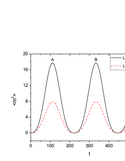
Figure 1: (Color online) Second moment $\langle m^{2}\rangle_{t}$ of the harmonic distribution versus time $t$ for the Dicke model at $\lambda=\lambda_{c}-10^{-4}$, $\lambda_{0}=\lambda_{c}-10^{-3}$ (solid curve) and $\lambda_{0}=\lambda_{c}-7\times 10^{-4}$ (dashed curve). Hereafter we set in numerical calculations $\omega=\omega_{0}=1$.

Next we consider the amplitude of the oscillations of the number of harmonics. We study the maximum value of $\langle m^{2}\rangle_{t}$ in Eq. (16), which is determined by the functions $\mathcal{F}(m,t_{p})$. Substituting Eq. (29) into Eq. (17), we obtain

$$\mathcal{F}(m,t_{p})=\sum\limits_{n\geq 0}\Big{|}\sum\limits_{\mu\nu}(-1)^{(\mu-\nu)/2}K_{\mu\nu}^{nm}\Big{|}^{2}.$$ (31)

Therefore, the amplitude of $\langle m^{2}\rangle_{t}$, denoted by $A_{p}$, is obtained from the summation of the terms $K_{\mu\nu}^{nm}$, with weights $(-1)^{(\mu-\nu)/2}$. As discussed in Appendix A, the quantities $K_{\mu\nu}^{nm}$ are in both phases functions of the ratio

$$\eta=\frac{\lambda-\lambda_{c}}{\lambda_{0}-\lambda_{c}}.$$ (32)

Therefore, $A_{p}$ depends only on the ratio $\eta$ and not on $\lambda$ and $\lambda_{0}$ separately. This property (illustrated in Fig. 2) is in agreement with the scaling derived in Ref. QPTscaling for metric quantities for QPTs with a single bosonic zero mode at the critical point. As shown in Fig. 2, the dependence of $A_{p}$ on $\eta$ can be well fitted by the curve $A_{p}=a|\eta|^{b}$ and since $b$ is negative, $A_{p}$ diverges when $|\eta|$ goes to zero.

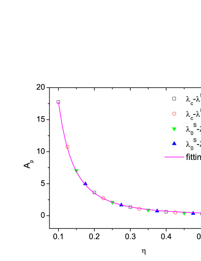
Figure 2: (Color online) Dependence of the amplitude $A_{p}$ on $\eta$ for different values of $|\lambda_{c}-\lambda_{0}|$ and $|\lambda_{c}-\lambda|$. Open symbols (with the superscript $N$ on $\lambda_{0}$) stand for the normal phase and closed symbols (superscript $S$) for the superradiant phase. The solid fitting curve is given by $A_{p}=a|\eta|^{b}$, with $a=0.083$ and $b=-2.3$.

A complete characterization of the harmonics dynamics is obtained by means of the harmonic probability distribution

$$Q(m,t)=\frac{\mathcal{F}(m,t)}{\sum\limits_{m\geq 0}\mathcal{F}(m,t)}.$$ (33)

Numerical simulations given in Fig. 3 for $t=t_{p}$ show that $Q$ decreases exponentially with increasing $m$, while, for a given $m$, the smaller the quantity $|\eta|$ is, the larger the value of $Q$. This latter behavior is in agreement with the fact that $A_{p}$ diverges when $\eta\to 0$. Since the distribution $Q(m,t_{p})$ decrease with $m$ exponentially, we can conclude that the quantity $\sqrt{\langle m^{2}\rangle_{t_{p}}}$ provides a good estimate of the number of harmonics developed up to the time $t_{p}$ and can be considered as a suitable measure of the complexity of the Wigner function at this time.

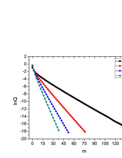
Figure 3: (Color online) Variation of $\ln Q$ with $m$ for $\lambda_{c}-\lambda=0.01$ and the harmonics distribution computed at the times $t_{p}$ corresponding to the maximum value of $\langle m^{2}\rangle_{t}$.

Finally, we discuss our numerical simulations for the time evolution of the number of harmonics of the Wigner function for times $t$ much shorter than the period $T$. Previous studies show that $\langle m^{2}\rangle_{t}$ is proportional to $t^{2}$ in the integrable regime of a single-particle system Benenti09 and grows exponentially in the integrable regime of a many-body system Vinitha10 . In our model, we found, both in the normal and in the superradiant phases, that $\langle m^{2}\rangle_{t}$ increases as $t^{2}$ within an initial period of time (see Fig. 4). For longer times (but still much smaller than $T$), $\langle m^{2}\rangle_{t}$ increases faster than $t^{2}$ in both phases. Further discussion about these behaviors of the number of harmonics will be given in the following section, where the relation between this quantity and the LE is discussed.

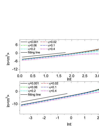
Figure 4: (Color online) Dependence of $\langle m^{2}\rangle_{t}$ on $t$ for $\lambda_{c}-\lambda_{0}=10^{-2}$ and $\eta$ between $0.4$ and $0.001$. The top panel is for the normal phase and the bottom panel is for the superradiant phase. The short solid straight lines indicate the $t^{2}$ behavior.

IV Lochmidt echo and fidelity for the Dicke model at QPT

The divergence of the number of harmonics developed by dynamics when approaching the critical point is a consequence of the fact that a small difference in the controlling parameter leads to a dramatic change of the wave function in the vicinity of a QPT. It is therefore interesting to compare the behavior of the number of harmonics with two other metric quantities, namely, the quantum Loschmidt echo and the fidelity.

The so-called quantum Loschmidt echo gives a measure to the stability of the quantum motion under slight variation of the Hamiltonian peres84 ; nie2000 ; ben2004 . It is defined by $M_{L}(t)=|m(t)|^{2}$, where

$$m_{L}(t)=\langle\Psi_{0}|{\rm exp}(i\hat{H}t/\hbar)\exp(-i\hat{H}^{\prime}t/\hbar)|\Psi_{0}\rangle.$$ (34)

Here $|\Psi_{0}\rangle$ is the initial state, $\hat{H}=\hat{H}^{\prime}+\varepsilon\hat{V}$, and $\varepsilon$ is a small parameter. Extensive investigations have been performed in recent years to understand the decaying behaviors of the LE jal2001 ; jac2001 ; cer2002 ; jac2002 ; cuc2002 ; STB03 ; wan2005 ; VH03 ; pro2002t ; pro2002 ; wan2004 ; wang2005 ; wan2007 ; BC02 ; Gorin-rep ; jacquodreport ; Wang10 . In chaotic systems, roughly speaking, the LE has a Gaussian decay peres84 below a perturbative border and has an exponential decay $M_{L}(t)\propto\exp(-\Gamma t)$ above the border. In the latter case, for intermediately strong perturbation cer2002 ; pro2002 $\Gamma$ is given by the half-width of the local spectral density of states and for relatively strong perturbation it is perturbation independent jal2001 ; STB03 ; wang2005 . In integrable systems with one degree of freedom, the LE has a Gaussian decay, followed after a transient region by a power-law decay wan2007 . In contrast, in integrable systems with many degrees of freedom the LE has an exponential decay Wang10 .

In our study of the LE, we take $\hat{H}=\hat{H}(\lambda)$ and $\hat{H}^{\prime}=\hat{H}(\lambda_{0})$, with $\hat{H}(\lambda)$ the Hamiltonian for the Dicke model and $\varepsilon=\lambda-\lambda_{0}$. Moreover, we choose the initial state to be the ground state $|\Phi_{0}(\lambda_{0})\rangle$ of $\hat{H}(\lambda_{0})$, so that the LE is in fact a survival probability. From Eq.(34) we obtain

$$M_{L}(t)=\left|\sum_{\mu}\left|\langle\Phi_{0}(\lambda_{0})|\Phi_{\mu}(\lambda)\rangle\right|^{2}e^{iE_{\mu}(\lambda)t}\right|^{2}.$$ (35)

Then, substituting Eq. (47) into Eq. (35), the LE can be written as

$$M_{L}(t)=\Big{|}\sum_{\mu}|C_{\mu}^{0}|^{2}e^{iE_{\mu}t}\Big{|}^{2},$$ (36)

where $C_{\mu}^{0}$ is defined in Eq.(47) of Appendix A. Using arguments similar to those given in Sec. III.2, one finds that the LE is also an oscillating function of time with the same period $T=\pi/e_{1}({\lambda})$ as for the number of harmonics. Moreover, $M_{L}(t)$ takes its minimum values, denoted by $M_{p}$, at the same times $t_{p}$ corresponding to the maximum values of the number of harmonics. As shown in Ref. QPTscaling (see Fig. 3 therein), the quantity $M_{p}$ is a function of the scaling parameter $\eta$ only,

$$M_{p}=\frac{2\sqrt{\eta}}{1+\eta}.$$ (37)

The analytical derivation of this formula is here provided in Appendix B.

Recent investigations show that the LE may be employed to characterize QPTs since it has been found to have extra-fast decay in the vicinity of the critical points Quan06 ; LE-qpt ; Rossini07 ; Peng08 ; Zhang09 ; Wang10 . Furthermore, as shown in Refs. Sokolov08 ; Benenti09 , the number of harmonics of the Wigner function may be connected to the LE. For example, in a single-particle system, to the lowest order in $\varepsilon$, the two quantities have the relation

$$M_{L}(t)\simeq 1-\frac{1}{2}\varepsilon^{2}\langle{m}^{2}\rangle_{t}.$$ (38)

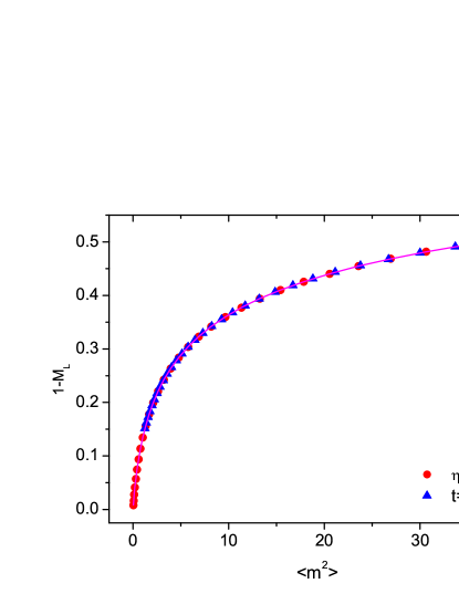
Figure 5: (Color online) Plot of $1-M_{L}$ vs the number of harmonics of the Wigner function $\langle m^{2}\rangle_{t}$. Circles denote $\eta=0.001$ and $\lambda_{0}=\lambda_{c}-0.01$, with the time $t$ varying from 1 to 25. Triangles denote $t=35$ and $\lambda_{0}=\lambda_{c}-0.005$, with $\eta$ varying from 0.001 to 0.3. The solid curve indicates the fitting function $1-M_{L}=\langle m^{2}\rangle_{t}/[3.5+\langle m^{2}\rangle_{t}+3(\langle m^{2}\rangle_{t})^{2/3}]$.

In order to find the relation between the number of harmonics of the Wigner function and the LE in the Dicke model, we have performed numerical simulations. We have found that there exists a one-to-one correspondence between the two quantities, as shown in Fig.5. That is, for different values of $\eta$ and $t$, the LE shows the same dependence on $\langle m^{2}\rangle_{t}$. Specifically, the following fitting function has been found to work well:

$$M_{L}=\frac{a+b(\langle m^{2}\rangle_{t})^{2/3}}{a+\langle m^{2}\rangle_{t}+b(\langle m^{2}\rangle_{t})^{2/3}},$$ (39)

with fitting parameters $a=3.5$ and $b=3.0$. For short times $t$ such that $[\langle m^{2}\rangle_{t}+b(\langle m^{2}\rangle_{t})^{2/3}]\ll a$, Eq. (39) gives

$$M_{L}(t)\simeq 1-\frac{1}{a}\,{\langle m^{2}\rangle_{t}}.$$ (40)

Equation (40) has a form similar to that in Eq. (38), however, one may note a major difference, i.e., the quantity $a$ in Eq. (40) is a fixed (fitting) parameter, but not a function of the perturbation strength $\varepsilon$. The dependence on $\varepsilon$ in (40) is contained only in $\langle m^{2}\rangle_{t}$ and we found numerically that $\langle m^{2}\rangle_{t}\propto\varepsilon^{2}$ for small $\varepsilon$.

In the Dicke model, it is known that the LE has an initial Gaussian decay Wang10 ; QPTscaling . Then Eq. (40) implies that the number of harmonics $\langle m^{2}\rangle_{t}$ should increase as $t^{2}$ within an initial period, in agreement with our numerical results (see Fig. 4) as well as with previous results for integrable single-particle systems Benenti09 . Beyond the initial Gaussian decay, after a transient region, the LE has been found Wang10 to show a $1/t$ decay for relatively long times (shorter than $T/2$) and for sufficiently small $\eta$. Consistently, Fig.4 shows that, in the corresponding situation, the number of harmonics increases faster than $t^{2}$. For $\langle m^{2}\rangle_{t}\gg 1$, the scaling in Eq. (39) reduces to $M_{L}\simeq b\langle m^{2}\rangle_{t}^{-1/3}$. Therefore, given that the LE $M_{L}\propto 1/t$ Wang10 , it gives $\langle m^{2}\rangle_{t}\propto t^{3}$. In fact, this is the reason we chose the exponent $2/3$ in the fitting in Eq. (39). However, we remark that, to see numerically the dependence $\langle m^{2}\rangle_{t}\propto t^{3}$, we would need much smaller values of $\eta$ than those accessible in our calculations.

Finally, for the sake of completeness, we briefly review results for another basic metric quantity used to characterize the occurrence of quantum phase transitions, namely, the fidelity

$$L_{p}=|\langle\Phi_{0}(\lambda_{0})|\Phi_{0}(\lambda)\rangle|,$$ (41)

which is given by the overlap of two ground states at different values $\lambda$ and $\lambda_{0}$ of the controlling parameter gu2010 ; zan2006 ; zho2008 ; zan2007 ; coz2007 ; cozz2007 ; buo2007 ; zana2007 . The dramatic change of the wave function at a QPT implies a fast decrease of $L_{p}$ in the neighborhood of the critical point. In the Dicke model, it has been found that $L_{p}\propto|\lambda_{0}-\lambda_{c}|^{1/8}$ for a sufficiently small $\varepsilon$ zan2006 . In Ref. QPTscaling we have shown that $L_{p}$ only depends on the scaling parameter $\eta$, with $L_{p}={\sqrt{2}\sqrt[8]{\eta}}/{\sqrt{\sqrt{\eta}+1}}$.

V Conclusions

In classical systems the growth rate of the number of harmonics is determined by the Lyapunov exponent Gong03 and complexity arises from the fact that the orbits of deterministic systems with positive Lyapunov exponent are unpredictable, with positive algorithmic complexity Ford ; AY81 . In the quantum realm, it was shown that the number of harmonics can be used to measure the complexity of single-particle systems, pure or mixed Sokolov08 , and to detect in the time domain the crossover from integrability to chaos Benenti09 . The effectiveness of such a measure for quantum many-body dynamics was illustrated for spin chains in Ref. Vinitha10 .

In this paper we have shown that the number of harmonics of the Wigner function is a suitable quantity to characterize quantum phase transitions. We have shown, in the case of the Dicke model, that there exists a one-to-one correspondence between the number of harmonics and the quantum Loschmidt echo such that both quantities can be equivalently used to characterize the quantum phase transition. We can conclude that the number of harmonics emerges as an extremely broad complexity quantifier.

Finally, we point out that our analysis could be extended to the case when several superradiant modes rather than a single one are formed at the transition, a phenomenon in analogy to the decay of collective excitations in highly excited heavy nuclei nuc1 ; nuc2 ; nuc3 ; nuc4 ; nuc5 ; nuc6 ; nuc7 .

Appendix A Some properties of the eigenstates of $\hat{H}(\lambda_{0})$ and $\hat{H}(\lambda)$ for the Dicke model

In this appendix we discuss some properties of the eigenstates of $\hat{H}(\lambda_{0})$ and $\hat{H}(\lambda)$ for the Dicke model. Let us first discuss the normal phase and write the lowest-mode annihilation operator $\hat{c}_{1}({\lambda_{0}})$ in terms of the creation and annihilation operators for the value $\lambda$ of the controlling parameter, namely,

$$\hat{c}_{1}({\lambda_{0}})=P_{1}\hat{c}_{1}(\lambda)^{\dagger}+P_{2}\hat{c}_{1}({\lambda}).$$ (42)

The coefficients $P_{1}$ and $P_{2}$ are given by Emary03

$$P_{1}=\frac{1}{2}\cos({r-r_{0}})\left(\sqrt{\frac{e_{1}(\lambda_{0})}{e_{1}(\lambda)}}-\sqrt{\frac{e_{1}(\lambda)}{e_{1}(\lambda_{0})}}\right),$$ (43)

$$P_{2}=\frac{1}{2}\cos({r-r_{0}})\left(\sqrt{\frac{e_{1}(\lambda_{0})}{e_{1}(\lambda)}}+\sqrt{\frac{e_{1}(\lambda)}{e_{1}(\lambda_{0})}}\right),$$ (44)

where $2{r}=\arctan\left[4\lambda\sqrt{\omega\omega_{0}}/(\omega_{0}^{2}-\omega^{2})\right]$. In the limit of small $\varepsilon=\lambda-\lambda_{0}$, $\cos({r-r_{0}})\approx 1$.

In the close neighborhood of the critical point $\lambda_{c}$, from Eq. (25) one gets

$$e_{1}({\lambda}) \simeq \left[\frac{8\lambda_{c}(\lambda_{c}-\lambda)\omega\omega_{0}}{\omega_{0}^{2}+\omega^{2}}\right]^{1/2}.$$ (45)

Then it is seen that $e_{1}({\lambda_{0}})/e_{1}({\lambda})\simeq(1/\eta)^{1/2}$, with the scaling parameter $\eta=(\lambda-\lambda_{c})/(\lambda_{0}-\lambda_{c})$. Using this result, we see that

$$P_{1}\simeq\frac{1}{2}\left(\frac{1}{\sqrt[4]{\eta}}-\sqrt[4]{\eta}\right),\ \ \ P_{2}\simeq\frac{1}{2}\left(\frac{1}{\sqrt[4]{\eta}}+\sqrt[4]{\eta}\right),$$ (46)

hence $P_{1}$ and $P_{2}$ are, close to the QPT, functions of the ratio $\eta$ only.

We also discuss some properties of the expanding coefficients of $|\Phi_{n}(\lambda_{0})\rangle$ in the basis $|\Phi_{\mu}(\lambda)\rangle$,

$$|\Phi_{n}(\lambda_{0})\rangle=\sum_{\mu}C_{\mu}^{n}|\Phi_{\mu}(\lambda)\rangle.$$ (47)

Let us write the coefficients in the form of vectors, i.e., $\mathbf{C}^{n}\equiv\{C_{0}^{n},C_{1}^{n},C_{2}^{n},\ldots\}$. We note that

$$\hat{c}_{1}({\lambda_{0}})|\Phi_{0}(\lambda_{0})\rangle = 0,$$ (48)

$$\hat{c}_{1}^{\dagger}({\lambda_{0})}|\Phi_{n}(\lambda_{0})\rangle = \sqrt{n+1}\ |\Phi_{n+1}(\lambda_{0})\rangle.$$ (49)

Substituting Eqs. (42) and (47) (for $n=0$) into Eq. (48), we obtain

$$C_{\mu}^{0} = \frac{-P_{1}\sqrt{\mu-1}}{P_{2}\sqrt{\mu}}\,C_{\mu-2}^{0}.$$ (50)

Then, substituting Eqs. (42) and (47) into Eq. (49), we find

$$\mathbf{C}^{n}=\frac{1}{\sqrt{n!}}\,\mathbf{C}^{0}(\mathbf{X})^{n},$$ (51)

where $\mathbf{X}$ is a symmetric triple-diagonal matrix

$$\mathbf{X}=\left(\begin{array}[]{cccc}0&P_{2}&&\\ P_{1}&0&\sqrt{2}P_{2}&\\ &\sqrt{2}P_{1}&0&\sqrt{3}P_{2}\\ &&\sqrt{3}P_{1}&\ddots\\ \end{array}\right).$$ (52)

Next, we discuss the superradiant phase. Similar to Eq. (42), we write

$$\hat{c}_{1}({\lambda_{0}})=P_{1}^{\prime}\hat{c}_{1}(\lambda)^{\dagger}+P_{2}^{\prime}\hat{c}_{1}({\lambda}),$$ (53)

where

$$P^{\prime}_{1}=\frac{1}{2}\cos({r^{\prime}-r^{\prime}_{0}})\left(\sqrt{\frac{e_{1}^{\prime}(\lambda_{0})}{e_{1}^{\prime}(\lambda)}}-\sqrt{\frac{e_{1}^{\prime}(\lambda)}{e_{1}^{\prime}(\lambda_{0})}}\right),$$ (54)

$$P^{\prime}_{2}=\frac{1}{2}\cos({r^{\prime}-r^{\prime}_{0}})\left(\sqrt{\frac{e_{1}^{\prime}(\lambda_{0})}{e_{1}^{\prime}(\lambda)}}+\sqrt{\frac{e_{1}^{\prime}(\lambda)}{e_{1}^{\prime}(\lambda_{0})}}\right).$$ (55)

Here $2{r^{\prime}}=\arctan\left[2\omega\omega_{0}{\kappa^{2}}/(\omega_{0}^{2}-{\kappa^{2}}\omega^{2})\right]$, with $\cos({r^{\prime}-r^{\prime}_{0}})\approx 1$ for small $\varepsilon$. From Eq. (27), one obtains

$$e_{1}^{\prime}(\lambda)\simeq\left[\frac{16(\lambda-\lambda_{c})(\lambda+\lambda_{c})(\lambda^{2}+\lambda^{2}_{c})}{\omega^{2}+\omega_{0}^{2}}\right]^{1/2}.$$ (56)

As a result, $e_{1}^{\prime}(\lambda_{0})/e_{1}^{\prime}(\lambda)\simeq(1/\eta)^{1/2}$, where $(\lambda_{0}+\lambda_{c})(\lambda^{2}_{0}+\lambda^{2}_{c})\simeq(\lambda+\lambda_{c})(\lambda^{2}+\lambda^{2}_{c})$ has been used in the neighborhood of the critical point. Then $P_{1}^{\prime}$ and $P_{2}^{\prime}$ are also functions of the ratio $\eta$ only. Moreover, Eq. (51) also holds in the superradiant phase.

From Eq. (50) we see that the $\mu$th coordinate of $\mathbf{C}^{n}$ is coupled to the $(\mu\pm 2)$th coordinates only, hence $C_{\mu}^{0}$ with even and odd $\mu$ are not connected. The continuity of the ground state of $H(\lambda)$ with respect to variation of $\lambda$ implies that $C_{0}^{0}$ is considerably large at least in the case of $\lambda\simeq\lambda_{0}$. Therefore, in the study of ground states, only even numbers $\mu$ should contribute significantly in Eq. (47). Then $K_{\mu\nu}^{nm}$ in Eq. (18) can be written as

$$K_{\mu\nu}^{nm}=(C^{n+m}_{\mu})^{\ast}C^{0}_{\mu}(C^{0}_{\nu})^{\ast}C^{n}_{\nu},$$ (57)

with even numbers $\mu$ and $\nu$.

Appendix B Derivation of Eq. (37)

Following arguments similar to those given in Sec. III.2 for the times at which the number of harmonics of the Wigner function takes the local-maximum values, it is seen that the LE in the Dicke model takes its locally lowest values $M_{p}$ at the same times $t_{p}$. Therefore, we can compute $M_{p}$ by Eq. (36) with $t=t_{p}$ and obtain

$$M_{p}=\left|\sum_{\mu}(-1)^{\mu/2}\left|C_{\mu}^{0}\right|^{2}\right|^{2},$$ (58)

with $\mu$ an even integer number. From Eq. (50) and the normalization condition, we obtain

$$\left|C_{\mu}^{0}\right|^{2}=\frac{\mathcal{P}^{\mu/2}\mathcal{D}_{\mu}}{\sum_{\mu}\mathcal{P}^{\mu/2}\mathcal{D}_{\mu}},$$ (59)

where $\mathcal{P}=(P_{1}/P_{2})^{2}$ and $\mathcal{D}_{\mu}=(\mu-1)!!/(\mu)!!$. Noticing that

$$\sum_{\mu}\mathcal{P}^{\mu/2}\frac{(\mu-1)!!}{(\mu)!!} = \frac{1}{\sqrt{1-\mathcal{P}}},$$ (60)

$$\sum_{\mu}(-1)^{\mu/2}\mathcal{P}^{\mu/2}\frac{(\mu-1)!!}{(\mu)!!} = \frac{1}{\sqrt{1+\mathcal{P}}},$$ (61)

we get

$$M_{p}=\frac{1-\mathcal{P}}{1+\mathcal{P}}.$$ (62)

Then, making use of Eq. (46), we have

$$\mathcal{P}=\left(\frac{1-\sqrt{\eta}}{1+\sqrt{\eta}}\right)^{2}.$$ (63)

Substituting this equation into Eq. (62), we finally obtain (37).

References

- (1) B. V. Chirikov, F. M. Izrailev, and D. L. Shepelyansky, Sov. Sci. Rev. C 2, 209 (1981).
- (2) Y. Gu, Phys. Lett. A 149, 95 (1990).
- (3) J. Ford, G. Mantica, and G. H. Ristow, Physica D 50, 493 (1991).
- (4) A. K. Pattanayak and P. Brumer, Phys. Rev. E 56, 5174 (1997).
- (5) J. Gong and P. Brumer, Phys. Rev. A 68, 062103 (2003).
- (6) V. V. Sokolov, O. V. Zhirov, G. Benenti, and G. Casati, Phys. Rev. E 78, 046212 (2008).
- (7) G. Benenti and G. Casati, Phys. Rev. E 79, 025201 (2009).
- (8) V. V. Sokolov and O. V. Zhirov, Europhys. Lett. 84, 30001 (2008).
- (9) V. Balachandran, G. Benenti, G. Casati, and J. Gong, Phys. Rev. E 82, 046216 (2010).
- (10) G. Casati, I. Guarneri, and J. Reslen, Phys. Rev. E 85, 036208 (2012).
- (11) G. Benenti, G. G. Carlo, and T. Prosen, Phys. Rev. E 85, 051129 (2012).
- (12) P. Zanardi and N. Paunković, Phys. Rev. E 74, 031123 (2006).
- (13) P. Zanardi, M. Cozzini and P. Giorda, J. Stat. Mech. (2007) L02002.
- (14) P. Zanardi, H. T. Quan, X. Wang and C. P. Sun, Phys. Rev. A 75, 032109 (2007).
- (15) M. Cozzini, P. Giorda and P. Zanardi, Phys. Rev. B 75, 014439 (2007).
- (16) M. Cozzini, R. Ionicioiu and P. Zanardi, Phys. Rev. B 76, 104420 (2007).
- (17) P. Buonsante and A. Vezzani, Phys. Rev. Lett. 98, 110601 (2007).
- (18) L. C. Venuti and P. Zanardi, Phys. Rev. Lett. 99, 095701 (2007)
- (19) H. Q. Zhou and J. P. Barjaktarevič, J. Phys. A: Math. Theor. 41, 412001 (2008).
- (20) T. Liu, Y. Y. Zhang, Q. H. Chen and K. L. Wang, Phys. Rev. A 80, 023810 (2009).
- (21) S. J. Gu, Int. J. Mod. Phys. B 24, 4371 (2010)
- (22) M. M. Rams and B. Damski, Phys. Rev. Lett. 106, 055701 (2011).
- (23) A. Peres, Phys. Rev. A 30, 1610 (1984)
- (24) M. A. Nielsen and I. L. Chuang, Quantum Computation and Quantum Information (Cambridge University Press, Cambridge, 2000).
- (25) G. Benenti, G. Casati, and G. Strini, Principles of Quantum Computation and Information, Vol. I: Basic concepts (World Scientific, Singapore, 2004); Principles of Quantum Computation and Information, Vol. II: Basic tools and special topics (World Scientific, Singapore, 2007).
- (26) R. A. Jalabert and H. M. Pastawski, Phys. Rev. Lett. 86, 2490 (2001).
- (27) Ph. Jacquod, P. G. Silvestrov, and C. W. J. Beenakker, Phys. Rev. E 64, 055203(R) (2001).
- (28) N. R. Cerruti and S. Tomsovic, Phys. Rev. Lett. 88, 054103 (2002).
- (29) Ph. Jacquod, I. Adagideli, and C. W. J. Beenakker, Phys. Rev. Lett. 89, 154103 (2002).
- (30) F. M. Cucchietti, C. H. Lewenkopf, E. R. Mucciolo, H. M. Pastawski, and R. O. Vallejos, Phys. Rev. E 65, 046209 (2002).
- (31) T. Prosen, Phys. Rev. E 65, 036208 (2002).
- (32) T. Prosen and M. Žnidarič, J. Phys. A: Math. Gen. 35, 1455 (2002).
- (33) G. Benenti and G. Casati, Phys. Rev.E 65, 066205 (2002).
- (34) J. Vaníček and E. J. Heller, Phys. Rev. E 68, 056208 (2003).
- (35) P. G. Silvestrov, J. Tworzydło, and C. W. J. Beenakker, Phys. Rev. E 67, 025204(R) (2003).
- (36) W.-G. Wang, G. Casati and B. Li, Phys. Rev. E 69, 025201(R) (2004).
- (37) W.-G. Wang and B. Li Phys. Rev. E 71, 066203 (2005).
- (38) W.-G. Wang, G. Casati, B. Li, and T. Prosen, Phys. Rev. E 71, 037202 (2005).
- (39) W.-G. Wang, G. Casati, and B. Li, Phys. Rev. E 75, 016201 (2007).
- (40) T. Gorin, T. Prosen, T. H. Seligman, and M. Žnidarič, Phys. Rep. 435, 33 (2006).
- (41) Ph. Jacquod and C. Petitjean, Adv. Phys. 58, 67 (2009).
- (42) W.-G. Wang, P. Qin, L. He, and P. Wang, Phys. Rev. E 81, 016214 (2010).
- (43) V. Bargmann, Commun. Pure Appl. Math. 14, 187 (1961).
- (44) R. J. Glauber, Phys. Rev. 131 2766 (1963).
- (45) G. S. Agarwal and E. Wolf, Phys. Rev. D 2, 2161 (1970).
- (46) The number of harmonics has been more precisely defined in Ref. Vinitha10 in terms of an entropic measure. However, for the purposes of the present paper it is sufficient to consider the second moment , which, as we will show, leads to a reliable estimate of the number of harmonics for the Dicke model close to its QPT.
- (47) J. Schwigner, Phys. Rev. 91, 728 (1953).
- (48) C. Emary and T. Brandes, Phys. Rev. E 67, 066203 (2003).
- (49) W.-G. Wang, P. Qin, Q. Wang, G. Benenti, and G. Casati, Phys. Rev. E 86, 021124 (2012).
- (50) H. T. Quan, Z. Song, X. F. Liu, P. Zanardi, and C. P. Sun, Phys. Rev. Lett. 96, 140604 (2006).
- (51) Z. G. Yuan, P. Zhang, and S. S. Li, Phys. Rev. A 75, 012102 (2007); Y. C. Li and S. S. Li, ibid. 76, 032117 (2007).
- (52) D. Rossini, T. Calarco, V. Giovannetti, S. Montangero, and R. Fazio, Phys. Rev. A 75, 032333 (2007).
- (53) J. Zhang, X. Peng, N. Rajendran, and D. Suter, Phys. Rev. Lett. 100, 100501 (2008).
- (54) J. Zhang, F. M. Cucchietti, C. M. Chandrashekar, M. Laforest, C. A. Ryan, M. Ditty, A. Hubbard, J. K. Gamble, and R. Laflamme, Phys. Rev. A 79, 012305 (2009).
- (55) J. Ford, Phys. Today 36(4), 40 (1983).
- (56) V. M. Alekseev and M. V. Yakobson, Phys. Rep. 75, 290 (1981).
- (57) V. V. Sokolov and V. G. Zelevinsky, Phys. Lett. 202, 10 (1988).
- (58) V. V. Sokolov and V. G. Zelevinsky, Nucl. Phys. A 504, 562 (1989).
- (59) V. V. Sokolov and V. G. Zelevinsky, Ann. Phys. (N.Y.) 216, 323 (1992).
- (60) F. M. Izrailev, D. Saher, and V. V. Sokolov, Phys. Rev. E 49, 130 (1994).
- (61) N. Lehmann, D. Saher, V. V. Sokolov, and H.-J. Sommers, Nucl. Phys. A 582, 223 (1995).
- (62) G. E. Mitchell, A. Richter, and H. A. Weidenmüller, Rev. Mod. Phys. 82, 2845 (2010).
- (63) N. Auerbach and V. Zelevinsky, Rep. Prog. Phys. 74, 106301 (2011).