Geometrically induced phase transitions in two-dimensional dumbbell-shaped domains

Abstract.

We continue the analysis, started in [16], of a two-dimensional non-convex variational problem, motivated by studies on magnetic domain walls trapped by thin necks. The main focus is on the impact of extreme geometry on the structure of local minimizers representing the transition between two different constant phases. We address here the case of general non-symmetric dumbbell-shaped domains with a small constriction and general multi-well potentials. Our main results concern the existence and uniqueness of non-constant local minimizers, their full classification in the case of convex bulks, and the complete description of their asymptotic behavior, as the size of the constriction tends to zero.

1. Introduction

In this paper we continue the study started in [14, 16] of the local minimizers of the following non-convex energy functional

$$F(u,\Omega_{\varepsilon})=\frac{1}{2}\int_{\Omega_{\varepsilon}}|\nabla u|^{2}\,dx+\int_{\Omega_{\varepsilon}}W(u)\,dx,$$ (1.1)

where $\Omega_{\varepsilon}\subset\mathbb{R}^{n}$ is a dumbbell shaped domain with a small neck (see Figure 1), $W(\cdot)$ is a multi-well potential, and $\varepsilon\ll 1$ is a small parameter related to the size of the neck.

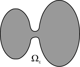
Figure 1. A dumbbell-shaped domain $\Omega_{\varepsilon}$.

We recall that a physical motivation comes from the investigation of the so-called geometrically constrained walls and the magnetoresistance properties of thin films with a small constriction. Indeed, if the thin film has cross section along the $xy$-plane given by a domain as in Figure 1, and the magnetization $m$ is allowed to vary only in the $yz$-plane (see Figure 2); i.e.,

$$m=(0,\cos u,\sin u),$$

with preferred directions $m=(0,\pm 1,0)$ (this assumption correspond to the case of uniaxial ferromagnet), then the magnetostatic interaction can be ignored and the stable magnetic structures are described by the local minimizers of a non-convex energy of the form (1.1), with $W(u)\approx\sin^{2}u$.

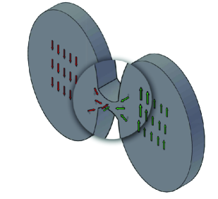
Figure 2. A thin micromagnetic film, with the arrows representing the magnetization. The magnified region is the magnetic domain wall.

One then wants to study the nonconstant local minimizers of (1.1) representing the transition from the constant state $(0,-1,0)$ in one bulk to the constant state $(0,1,0)$ in the other bulk.

Following the pioneering work by Bruno [2], the study of geometrically constrained walls has attracted the interest of the physical community from both the theoretical [15, 5] and the experimental points of view [6, 13, 18, 19]. Bruno noticed that when the size of the constriction becomes very small the neck will be the preferred location for a domain wall, that is, the transition layer between two regions of (almost) constant magnetization. He also observed that under these circumstances the impact of the geometry of the neck on the structure of the wall profile becomes dominant and produces a limiting behavior that is independent of the material parameters (whence the name of geometrically constrained walls or geometrically induced phase transitions).

When the size $\varepsilon$ of the constriction is very small, we may regard the neck as a singular perturbation of the domain given by the disjoint union of the two bulks. There exists an extensive mathematical literature devoted to a study of the properties of solutions to nonlinear partial differential equations in singularly perturbed domains, see for instance [1, 4, 7, 8, 9, 10, 11, 12, 14, 16, 17]. Apart from the directly relevant papers [14, 16] the closest in spirit to this work is that of Jimbo. In the series of papers [10, 11, 12] he uses PDE methods to study the asymptotic behaviour of the solutions of semilinear elliptic problems for $n$-dimensional dumbbell shaped domain ($n\geq 2$) with a rotationally symmetric neck of fixed length and shrinking in the radial direction.

As already mentioned, our work is closely related to [14, 16]. In [14] a rigorous study of geometrically constrained walls was undertaken in the three-dimensional case. The authors constructed a suitable family $u_{\varepsilon}$ of non-trivial local minimizers of $F(\cdot,\Omega_{\varepsilon})$ with the choice $W(u):=(u^{2}-1)^{2}$ and investigated their asymptotic behavior using variational methods and $\Gamma$-convergence arguments. This behavior was shown to strongly depend on the size of the neck, specifically on the ratio between the radius $\delta$ of the neck and its length $\varepsilon$. Three asymptotic regimes were identified, leading to three different limiting problems:

• the thin neck regime, corresponding to $\displaystyle\frac{\delta}{\varepsilon}\to 0$;

• the normal neck regime, corresponding to $\displaystyle\frac{\delta}{\varepsilon}\to l=cost$;

• the thick neck regime, corresponding to $\displaystyle\frac{\delta}{\varepsilon}\to\infty$.

The findings of [14] show that in the thin neck regime the wall profile is asymptotically confined inside the neck and its limiting one-dimensional behavior depends only on the geometry of the neck. This is the only regime where the one-dimensional ansatz considered in [2] turns out to be correct. Instead, in the normal neck regime the asymptotic profile is three-dimensional and spreads into the bulks. Finally, in the thick neck regime the asymptotic problem is independent of the neck geometry and the full transition between the two states of constant magnetization occurs outside of the neck.

The variational methods introduced in [14] do not apply to the two-dimensional case, where the logarithmic slow decay of the fundamental solution significantly affects the qualitative behavior of local minimizers. This problem was treated in [16] in the case when $\Omega_{\varepsilon}\subset\mathbb{R}^{2}$ is a dumbbell shaped domain symmetric with respect to the $y$-axis and $W$ is an even double-well potential with the two symmetric wells located at $-1$ and $1$ (and satisfying some additional structure assumptions of technical nature). More precisely, in [16] we have constructed a particular family $(u_{\varepsilon})$ of local minimizers, odd with respect to the $x$-variable, and asymptotically converging to $1$ on the right bulk and to $-1$ on the left bulk, and we studied their asymptotic behavior as $\varepsilon\to 0$. The result of this investigation shows that the two-dimensional case displayis a richer variety of asymptotic regimes. In particular, in addition to the normal and thick neck regimes, we found out that the thin neck regime subdivides into three further subregimes:

• the subcritical thin neck regime, corresponding to $\displaystyle\frac{\delta|\ln\delta|}{\varepsilon}\to 0$;

• the critical thin neck regime, corresponding to $\displaystyle\frac{\delta|\ln\delta|}{\varepsilon}\to l=const$;

• the supercritical thin neck regime, corresponding to $\displaystyle\frac{\delta|\ln\delta|}{\varepsilon}\to\infty$.

In all cases, the limiting behavior turns out to be nonvariational and can be described in terms of elliptic problems on suitable unbounded domains, with prescribed behavior at infinity. This is the reason why the approach introduced in [16] is based on PDE methods rather then $\Gamma$-convergence techniques. There, the main idea is to exploit the Maximum Principle in order to construct precise lower and upper barriers for the given local minimizers, which allow us to capture their asymptotic behavior. Nevertheless, these constructions heavily rely on the symmetry of $\Omega_{\varepsilon}$ and the fact that $u_{\varepsilon}=0$ on the middle vertical segment $\{x=0\}\cap\Omega_{\varepsilon}$.

The main questions left open in [16] are: (a) Is the constructed family $(u_{\varepsilon})$ the unique family of nontrivial local minimizer of $F_{\varepsilon}$ asymptotically connecting the constant states $-1$ and $1$? (b) Can the analysis of [16] be extended to the case of non-symmetric domains? We address these issues in the present paper.

We are now in a position to describe our results in more detail, referring to the next sections for the precise statements. We assume $\Omega_{\varepsilon}$ to be a dumbbell shaped domain consisting of two bulks $\Omega_{\varepsilon}^{l}=\Omega_{l}-(\varepsilon,0)$ and $\Omega_{\varepsilon}^{r}=\Omega_{r}+(\varepsilon,0)$ not necessarily symmetric and connected by a small neck $N_{\varepsilon}$. The dimensions of the neck are governed by two small parameters $\varepsilon$ and $\delta$, corresponding to its length and height, respectively. We consider general multi-well potentials $W$ of class $C^{2}$, with isolated wells. Our main findings can be summarized as follows:

1. (existence): we prove that for any pair $\alpha\neq\beta$ of wells of $W$, there exists a family $(u_{\varepsilon})$ of non-constant local minimizers of $F(\cdot,\Omega_{\varepsilon})$, which asymptotically connect the constant states $\alpha$ and $\beta$; i.e., $u_{\varepsilon}\approx\alpha$ on one bulk and $u_{\varepsilon}\approx\beta$ on the other, for $\varepsilon$ small enough;

2. (uniqueness): we show that for given $\alpha$, $\beta$, the corresponding family of non-constant local minimizers as in (1) is unique;

3. (classification): we show that the family of non-constant local minimizers considered in the previous items exhaust all the possible local minimizers of $F(\cdot,\Omega_{\varepsilon})$ for $\varepsilon$ small enough, provided that the bulks $\Omega^{l}$ and $\Omega^{r}$ are convex and regular enough;

4. (asymptotics): we identify the limiting behavior of the families of local minimizers considered in (1) and (2) in all the regimes determined by the scaling parameters $\varepsilon$ and $\delta$.

We will refer to the families of local minimizers described in (1) as families of nearly locally constant local minimizers. The proof of the existence is purely variational and adapts to the present setting an argument developed in [14]. In fact, the same argument could be used to establish the following general bridge principle: if $u^{l}$ and $u^{r}$ are isolated local minimizers of $F(\cdot,\Omega^{l})$ and $F(\cdot,\Omega^{r})$, respectively, then there exists a (unique) family $(u_{\varepsilon})$ of local minimizers of $F(\cdot,\Omega_{\varepsilon})$ such that $u_{\varepsilon}\approx u^{l}$ in the left bulk $\Omega_{\varepsilon}^{l}$ and $u_{\varepsilon}\approx u^{r}$ in $\Omega_{\varepsilon}^{r}$ for $\varepsilon$ small enough (see Remark 3.7). We remark that the non-convexity of $\Omega_{\varepsilon}$ is a necessary condition for the existence of non-constant local minimizers (see [3]).

The uniqueness follows from showing that the local minimizers $u_{\varepsilon}$ are in fact isolated $L^{1}$-local minimizer of $F(\cdot,\Omega_{\varepsilon})$. This observation is based on a second variation argument and requires one to carefully track the behavior of the first eigenvalue $\lambda_{\varepsilon}$ of $\partial^{2}F(\cdot,\Omega_{\varepsilon})$, as $\varepsilon\to 0$.

As shown in [3], if $\Omega$ is regular and convex, then all the stable critical points of $F(\cdot,\Omega)$ are constant. This fact, properly combined with the existence and uniqueness results described before, allows us to provide a complete classification of the stable critical points of $F(\cdot,\Omega_{\varepsilon})$ for $\varepsilon$ small enough, when the bulks $\Omega^{l}$ and $\Omega^{r}$ are convex and regular. See Theorem 3.12 for precise statement.

Finally, a few words are in order regarding the study of the asymptotic behavior of the local minimizers. As mentioned before, the methods and the constructions of [16] were heavily relying on the symmetry assumptions of both $\Omega_{\varepsilon}$ and the potential $W$. The lack of symmetry here is overcome by a careful estimate of the amount of energy $F(u_{\varepsilon},B_{\delta})$, which concentrates on small balls $B_{\delta}$ of size $\delta$ centered at points of the neck. This localization estimate, which is obtained by a blow-up argument, allows us to adapt (and in fact to simplify) some of the constructions of [16] and to extend all the results to general non-symmetric domains.

The paper is organized as follows. In Section 2 we formulate the problem and describe the assumptions on the domains $\Omega_{\varepsilon}$ and the potential $W$. In Section 3 we prove the existence and uniqueness of families of nearly locally constant local minimizers, and provide a complete classification of stable critical points in the case of regular convex bulks $\Omega^{l}$ and $\Omega^{r}$. Finally, Section 4 is devoted to the study of the asymptotic behavior of families of nearly locally constant local minimizers in the various regimes. We will work out the details only in the normal neck and critical thin neck regimes and only state the results in the remaining regimes, leaving the similar (and in fact easier proofs) to the interested reader.

2. Formulation of the problem

In this section we give the precise formulation of the problem. We start by describing the limiting domain. This will be the disjoint union

$$\Omega_{0}=\Omega^{l}\cup\Omega^{r}\,,$$

where $\Omega^{l}$ and $\Omega^{r}$ are bounded connected open sets of class $C^{1,\gamma}$ for some $\gamma\in(0,1)$, satisfying (see Figure 3):

• the origin $(0,0)$ belongs to both $\partial\Omega^{r}$ and $\partial\Omega^{l}$;

• $\Omega^{r}$ lies in the right half-plane $\{x>0\}$, while $\Omega^{l}$ lies in left half-plane $\{x<0\}$.

Finally, throughout the paper we will also make the following technical assumption:

• there exists $r_{0}>0$ such that $\partial\Omega^{r}\cap B_{2r_{0}}(0,0)$ and $\partial\Omega^{l}\cap B_{2r_{0}}(0,0)$ are flat and vertical.

Hypothesis (O3) is not really necessary for the analysis carried out in this paper. We decided to add it in order to avoid some technicalities that would distract from the main new ideas introduced here. All the results we are going to prove remain valid also without the additional assumption. Indeed, if (O3) does not hold, one can reduce to it by straightening the boundary through a suitable conformal change of variables and then construct the same barriers and test functions presented here, but with respect to the new variables (see, for instance, [16, Section 3]).

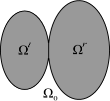
Figure 3. The limiting set $\Omega_{0}$.

The profile of the neck after rescaling is described by two functions $f_{1},f_{2}\,:\,[-1,1]\mapsto(0,+\infty)$ of class $C^{1,\gamma}$ and by the two small parameters $\varepsilon>0$ and $\delta=\delta(\varepsilon)>0$, which represent the scaling of length and height of the neck, respectively. As in [16], $\delta$ will always be considered as depending on $\varepsilon$, even though, for notational convenience, we will often omit to explicitly write such a dependence. We also assume throughout the paper that $\delta(\varepsilon)\to 0$ as $\varepsilon\to 0$. To describe the $\varepsilon$-domain, we set

$$\Omega_{\varepsilon}=\Omega_{\varepsilon}^{l}\cup N_{\varepsilon}\cup\Omega_{\varepsilon}^{r},$$ (2.1)

where

$$\Omega_{\varepsilon}^{r}:=\Omega^{r}+(\varepsilon,0)\,,\qquad\Omega_{\varepsilon}^{l}:=\Omega^{l}-(\varepsilon,0)$$ (2.2)

and

$$N_{\varepsilon}:=\Bigl{\{}(x,y)\,:\,|x|\leq\varepsilon,\,-\delta f_{2}\Bigl{(}\frac{x}{\varepsilon}\Bigr{)}<y<\delta f_{1}\Bigl{(}\frac{x}{\varepsilon}\Bigr{)}\Bigr{\}}$$ (2.3)

(see Figure 4).

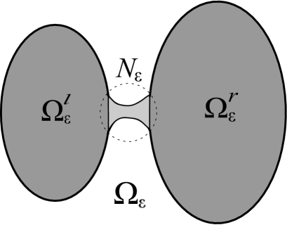
Figure 4. The dumbbell-shaped set $\Omega_{\varepsilon}$.

Note that

$$N_{\varepsilon}=\{(\varepsilon x,\delta y):(x,y)\in N\}\,,$$

where $N$ is the unscaled neck given by

$$N=\{(x,y):x\in[-1,1]\,,-f_{2}(x)<y<f_{1}(x)\}\,.$$ (2.4)

Finally, observe that $\Omega_{\varepsilon}$ is a Lipschitz domain.

The main focus of the paper is the study of a suitable class of nearly constant critical points of the energy functional

$$F(u,\Omega_{\varepsilon}):=\frac{1}{2}\int_{\Omega_{\varepsilon}}|\nabla u|^{2}\,dxdy+\int_{\Omega_{\varepsilon}}W(u)\,dxdy\,,$$

defined for all $u\in H^{1}(\Omega_{\varepsilon})$. Here, and throughout the paper, $W:\mathbb{R}\to\mathbb{R}$ is a multi-well potential with the following properties (see Figure 5):

• $W$ is of class $C^{2}$;

• the set

  $$V:=\{t\in\mathbb{R}:\,W^{\prime}(t)=0\text{ and }W^{\prime\prime}(t)>0\}$$ (2.5)

  contains at least two points.

Clearly, $V$ represents the set of wells of the potential $W$. A model case is of course given by $W(u):=(u-\alpha)^{2}(u-\beta)^{2}$.

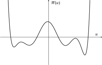
Figure 5. An example of a potential $W(u)$.

We recall that a function $u\in H^{1}(\Omega_{\varepsilon})$ is a critical point for $F(\cdot,\Omega_{\varepsilon})$ if it satisfies

$$\begin{cases}\Delta u=W^{\prime}(u)&\text{in $\Omega_{\varepsilon}$,}\\ \displaystyle\frac{\partial u}{\partial\nu}=0&\text{on $\partial\Omega_{\varepsilon}$,}\end{cases}$$ (2.6)

or, equivalently,

$$\int_{\Omega_{\varepsilon}}\nabla u\nabla\varphi\,dxdy+\int_{\Omega_{\varepsilon}}W^{\prime}(u)\varphi\,dxdy=0\qquad\text{for all }\varphi\in H^{1}(\Omega_{\varepsilon})\,.$$ (2.7)

Finally, it is convenient to extend the definition of $F$ to any subset $\Omega\subset\mathbb{R}^{2}$, by setting

$$F(u,\Omega):=\frac{1}{2}\int_{\Omega}|\nabla u|^{2}\,dxdy+\int_{\Omega}W(u)\,dxdy\,,$$ (2.8)

for all $u\in H^{1}(\Omega)$.

3. Nearly locally constant critical points

In this paper we are concerned with the existence and the asymptotic behavior of sequences of critical points that are nearly constant, according to the following definition.

Definition 3.1.

For $\varepsilon>0$ let $u_{\varepsilon}\in H^{1}(\Omega_{\varepsilon})$ be a critical point of $F(\cdot,\Omega_{\varepsilon})$. We say that the family $(u_{\varepsilon})$ is an admissible family of nearly locally constant critical points if

• there exists $\bar{\varepsilon}>0$ such that $\sup_{0<\varepsilon\leq\bar{\varepsilon}}\|u_{\varepsilon}\|_{\infty}=:\overline{M}<+\infty$;

• there exist constants $\alpha\neq\beta$ belonging to the set $V$ in (2.5) such that

  $$\|u_{\varepsilon}-\alpha\|_{L^{1}(\Omega^{l}_{\varepsilon})}\to 0\qquad\text{and}\qquad\|u_{\varepsilon}-\beta\|_{L^{1}(\Omega^{r}_{\varepsilon})}\to 0\,,$$ (3.1)

  as $\varepsilon\to 0^{+}$.

Remark 3.2.

Under additional assumptions on the potential $W$, condition (a) in the above definition is automatically satisfied. For instance, this is the case when $W$ satisfies:

• there exists $\overline{M}>0$ such that $W^{\prime}(t)>0$ if $t\geq\overline{M}$ and $W^{\prime}(t)<0$ if $t\leq-\overline{M}$.

Indeed, by the maximum principle one can show that any solution $u$ to (2.6) satisfies $|u|\leq\overline{M}$.

We will prove that nearly constant critical points are local minimizers of the energy functional for $\varepsilon$ small enough. Hence, they represent physically observable stable configurations.

Theorem 3.3.

Let $(u_{\varepsilon})$ be a family of critical points as in Definition 3.1. Then, there exist $\varepsilon_{0}>0$ and $\eta_{0}>0$ such that for $0<\varepsilon\leq\varepsilon_{0}$

$$F(v,\Omega_{\varepsilon})>F(u_{\varepsilon},\Omega_{\varepsilon})\qquad\text{for all $v\in H^{1}(\Omega_{\varepsilon})$ such that $0<\|v-u_{\varepsilon}\|_{L^{1}(\Omega_{\varepsilon})}\leq\eta_{0}$.}$$ (3.2)

Both $\varepsilon_{0}$ and $\eta_{0}$ depend only on the constants $\alpha$, $\beta$, and $\overline{M}$ appearing in Definition 3.1.

The proof the theorem borrows some ideas from [16, Lemma 2.2]. Before starting, we recall the following simple Poincaré inequality (see [16, Proof of Lemma 2.2-Step 2]).

Lemma 3.4.

There exists a constant $C_{1}>0$ independent of $\varepsilon$ such that

$$\int_{N^{+}_{\varepsilon}}|\nabla\varphi|^{2}\,dxdy\geq\frac{C_{1}}{\varepsilon^{2}}\int_{N^{+}_{\varepsilon}}|\varphi|^{2}\,dxdy$$

for all $\varphi\in H^{1}(N^{+}_{\varepsilon})$ satisfying $\varphi=0$ on $\{x=\varepsilon\}$, where $N^{+}_{\varepsilon}:=N_{\varepsilon}\cap\{x>0\}$.

Proof of Theorem 3.3.

We split the proof into theree steps.

Step 1. (Positive definiteness of the second variation) We start by assuming that there exists $M>0$ such that

$$|W^{\prime\prime}(t)|\leq M\qquad\text{for all $t\in\mathbb{R}$.}$$ (3.3)

Given $u$, $\varphi\in H^{1}(\Omega_{\varepsilon})$, and $\Omega\subset\Omega_{\varepsilon}$ we define the second variation of $F(\cdot,\Omega)$ at $u$ with respect to the direction $\varphi$ as

$$\partial^{2}F(u,\Omega)[\varphi]:=\frac{d^{2}}{dt^{2}}F(u+t\varphi,\Omega)|_{t=0}=\int_{\Omega}|\nabla\varphi|^{2}\,dxdy+\int_{\Omega}W^{\prime\prime}(u)\varphi^{2}dxdy\,.$$

Set $\Omega_{\varepsilon}^{+}:=\Omega_{\varepsilon}\cap\{x>0\}$. We claim that there exist $\eta^{+}_{0}>0$ (independent of $\varepsilon$) and $\varepsilon_{0}^{+}>0$ such that

$$\partial^{2}F(v,\Omega^{+}_{\varepsilon})[\varphi]\geq\frac{W^{\prime\prime}(\beta)}{2}\|\varphi\|^{2}_{L^{2}(\Omega^{+}_{\varepsilon})}\qquad\text{for all $\varphi\in H^{1}(\Omega_{\varepsilon}^{+})$}$$ (3.4)

provided that $\varepsilon\in(0,\varepsilon_{0}^{+})$ and $\|v-u_{\varepsilon}\|_{L^{1}(\Omega^{+}_{\varepsilon})}\leq\eta_{0}^{+}$. To this aim, we argue by contradiction by assuming that there exist $\varepsilon_{n}\to 0$ and $(v_{n})$ such that

$$\|v_{n}-u_{\varepsilon_{n}}\|_{L^{1}(\Omega^{+}_{\varepsilon_{n}})}\to 0$$ (3.5)

and for all $n\in\mathbb{N}$

$$\partial^{2}F(v_{n},\Omega^{+}_{\varepsilon_{n}})[\varphi]<\frac{W^{\prime\prime}(\beta)}{2}\|\varphi\|^{2}_{L^{2}(\Omega^{+}_{\varepsilon_{n}})}\qquad\text{for some $\varphi\in H^{1}(\Omega_{\varepsilon_{n}}^{+})$.}$$

Thus, if we set

$$\lambda^{+}_{n}:=\min\left\{\partial^{2}F(v_{n},\Omega_{\varepsilon}^{+})[\varphi]:\,\varphi\in H^{1}(\Omega_{\varepsilon}^{+}),\,\|\varphi\|_{L^{2}(\Omega_{\varepsilon}^{+})}=1\right\}\,,$$ (3.6)

we have

$$\liminf_{n\to+\infty}\lambda_{n}^{+}\leq\frac{W^{\prime\prime}(\beta)}{2}\,.$$ (3.7)

We may assume, without generality, that $\liminf_{n\to\infty}\lambda_{n}^{+}=\lim_{n\to\infty}\lambda_{n}^{+}$. Let $\varphi_{n}$ be a minimizer for the problem (3.6) corresponding to $\varepsilon_{n}$ and note that

$$\sup_{n}\|\varphi_{n}\|_{H^{1}(\Omega^{+}_{\varepsilon_{n}})}^{2}\leq 1+\sup_{n}(\lambda^{+}_{n}+\|W^{\prime\prime}(u_{\varepsilon_{n}})\|_{\infty})<+\infty\,.$$ (3.8)

Thus, in particular, there exists $\varphi\in H^{1}(\Omega^{r})$ and a subsequence (not relabeled) such that

$$\psi_{n}:=\varphi_{n}(\varepsilon_{n}+\cdot,\cdot)\rightharpoonup\varphi$$ (3.9)

weakly in $H^{1}(\Omega^{r})$. We claim that

$$\|\varphi\|_{L^{2}(\Omega^{r})}=1\,.$$ (3.10)

To this aim, extend $\varphi_{n}|_{\Omega_{\varepsilon_{n}}^{r}}$ to a function $\tilde{\varphi}_{n}\in H^{1}(\mathbb{R}^{2})$ in such a way that

$$\|\tilde{\varphi}_{n}\|_{H^{1}(\mathbb{R}^{2})}\leq C^{\prime}\|\varphi_{n}\|_{H^{1}(\Omega^{r}_{\varepsilon_{n}})}\,,$$

with $C^{\prime}$ independent of $n$, where we recall $\Omega^{r}_{\varepsilon_{n}}=\Omega^{r}+(\varepsilon,0)$. Note that this is possible due to the regularity of $\partial\Omega^{r}$.

Fix $p>2$. Then,

$$\int_{N^{+}_{\varepsilon_{n}}}\tilde{\varphi}_{n}^{2}\,dxdy\leq\Bigl{(}\int_{N^{+}_{\varepsilon_{n}}}\tilde{\varphi}_{n}^{p}\,dxdy\Bigr{)}^{\frac{2}{p}}|N_{\varepsilon_{n}}^{+}|^{1-\frac{2}{p}}\leq c_{p}\|\varphi_{n}\|^{2}_{H^{1}(\Omega^{+}_{\varepsilon})}|N_{\varepsilon_{n}}^{+}|^{1-\frac{2}{p}}\to 0\,,$$ (3.11)

where we used the imbedding of $H^{1}(\mathbb{R}^{2})$ into $L^{p}(\mathbb{R}^{2})$ and (3.8). Moreover,

$$\int_{N^{+}_{\varepsilon_{n}}}|\nabla\varphi_{n}|^{2}\,dxdy \geq\frac{1}{2}\int_{N^{+}_{\varepsilon_{n}}}|\nabla(\varphi_{n}-\tilde{\varphi}_{n})|^{2}\,dxdy-\int_{N^{+}_{\varepsilon_{n}}}|\nabla\tilde{\varphi}_{n}|^{2}\,dxdy$$ (3.12)

$$\geq\frac{C_{1}}{\varepsilon_{n}^{2}}\int_{N^{+}_{\varepsilon_{n}}}|\varphi_{n}-\tilde{\varphi}_{n}|^{2}\,dxdy-C_{2}\,,$$

where in the last inequality we have used Lemma 3.4 and again the fact that $\sup_{n}\|\tilde{\varphi}_{n}\|^{2}_{H^{1}(\mathbb{R}^{2})}\leq C_{2}<+\infty$ thanks to (3.8). Since the left-hand side of (3.12) is bounded, recalling (3.11), we deduce

$$\int_{N^{+}_{\varepsilon_{n}}}\varphi_{n}^{2}\,dxdy\to 0\,.$$ (3.13)

Thus, claim (3.10) follows from (3.9) observing that $\int_{\Omega^{r}}\psi^{2}_{n}\,dxdy=1-\int_{N^{+}_{\varepsilon_{n}}}\varphi_{n}^{2}\,dxdy$.

Set now $w_{n}(x,y):=v_{n}(x+\varepsilon_{n},y)$ and note that by (3.1)-(ii) and (3.5) we have $w_{n}\to\beta$ in $L^{1}(\Omega^{r})$. Thus, by lower semicontinuity and recalling also (3.6) and (3.9), we have

$$\liminf_{n\to\infty}\lambda_{\varepsilon_{n}}^{+} \geq\liminf_{n\to\infty}\int_{\Omega_{\varepsilon_{n}}^{r}}|\nabla\varphi_{n}|^{2}\,dxdy+\int_{\Omega^{+}_{\varepsilon_{n}}}W^{\prime\prime}(v_{n})\varphi_{n}^{2}dxdy$$

$$=\liminf_{n\to\infty}\int_{\Omega^{r}}|\nabla\psi_{n}|^{2}\,dxdy+\int_{\Omega^{r}}W^{\prime\prime}(w_{n})\psi_{n}^{2}dxdy$$

$$\geq\int_{\Omega^{r}}|\nabla\varphi|^{2}\,dxdy+W^{\prime\prime}(\beta)\int_{\Omega^{r}}\varphi^{2}dxdy\geq W^{\prime\prime}(\beta)\,,$$

where the equality is a consequence of (3.3) and (3.13), while the last inequality follows from the definition of $\lambda_{0}^{+}$ and (3.10). The above chain of inequalities contradicts (3.7) and completes the proof of (3.4). An entirely similar argument shows that there exist $\eta^{-}_{0}>0$ (independent of $\varepsilon$) and $\varepsilon_{0}^{-}>0$ such that

$$\partial^{2}F(v,\Omega^{-}_{\varepsilon})[\varphi]\geq\frac{W^{\prime\prime}(\alpha)}{2}\|\varphi\|^{2}_{L^{2}(\Omega^{-}_{\varepsilon})}\qquad\text{for all $\varphi\in H^{1}(\Omega_{\varepsilon}^{-})$}$$

provided that $\varepsilon\in(0,\varepsilon_{0}^{-})$ and $\|v-u_{\varepsilon}\|_{L^{1}(\Omega^{-}_{\varepsilon})}\leq\eta_{0}^{-}$, where $\Omega_{\varepsilon}^{-}:=\Omega_{\varepsilon}\cap\{x<0\}$. Thus, setting $\varepsilon_{0}:=\min\{\varepsilon_{0}^{-},\varepsilon_{0}^{+}\}$, $\eta_{0}:=\min\{\eta_{0}^{-},\eta_{0}^{+}\}$, and $\lambda_{0}:=\min\{W^{\prime\prime}(\alpha),W^{\prime\prime}(\beta)\}$, we may assert that

$$\partial^{2}F(u_{\varepsilon},\Omega_{\varepsilon})[\varphi]\geq\frac{\lambda_{0}}{2}\|\varphi\|^{2}_{L^{2}(\Omega_{\varepsilon})}\qquad\text{for all $\varphi\in H^{1}(\Omega_{\varepsilon})$}$$ (3.14)

provided that $\varepsilon\in(0,\varepsilon_{0})$ and $\|v-u_{\varepsilon}\|_{L^{1}(\Omega_{\varepsilon})}\leq\eta_{0}$.

Step 2. (Conclusion under assumption (3.3)) Assume (3.3). Fix $v\in H^{1}(\Omega_{\varepsilon})$ with $\|v-u_{\varepsilon}\|_{L^{1}(\Omega_{\varepsilon})}\leq\eta_{0}$ and set $f(t):=F(u_{\varepsilon}+t(v-u_{\varepsilon}),\Omega_{\varepsilon})$. Then, for $t\in(0,1)$ by (3.14) we have

$$f^{\prime\prime}(t)=\partial^{2}F(u_{\varepsilon}+t(v-u_{\varepsilon}),\Omega_{\varepsilon})[v-u_{\varepsilon}]\geq\frac{\lambda_{0}}{2}\|v-u_{\varepsilon}\|^{2}_{L^{2}(\Omega_{\varepsilon})}$$

provided that $\varepsilon\in(0,\varepsilon_{0})$. Hence, also recalling that $f^{\prime}(0)=0$ due to the criticality of $u_{\varepsilon}$, we deduce

$$F(v,\Omega_{\varepsilon}) =f(1)=f(0)+\int_{0}^{1}(1-t)f^{\prime\prime}(t)\,dt$$

$$\geq F(u_{\varepsilon},\Omega_{\varepsilon})+\frac{\lambda_{0}}{4}\|u_{\varepsilon}-v\|^{2}_{L^{2}(\Omega_{\varepsilon})}\,,$$

which yields the conlusion of the theorem under assumption (3.3)

Step 3. (The general case) We now remove the extra assumption (3.3). To this aim, let $\widetilde{W}:\mathbb{R}\to\mathbb{R}$ be a $C^{2}$ function such that

• $\widetilde{W}=W$ on $[-\overline{M},\overline{M}]$ where $\overline{M}$ is the constant appearing in condition (a) of Definition 3.1;

• $\widetilde{W}\leq W$ everywhere;

• $|\widetilde{W}^{\prime\prime}|\leq M$ everywhere, for some $M>0$.

For every $u\in H^{1}(\Omega_{\varepsilon})$ define

$$\widetilde{F}(u,\Omega_{\varepsilon}):=\frac{1}{2}\int_{\Omega_{\varepsilon}}|\nabla u|^{2}\,dx+\int_{\Omega_{\varepsilon}}\widetilde{W}(u)\,dx\,,$$

and note that

$$F(v,\Omega_{\varepsilon})\geq\widetilde{F}(v,\Omega_{\varepsilon})\quad\text{for all $v\in H^{1}(\Omega_{\varepsilon})$ and }\widetilde{F}(u_{\varepsilon},\Omega_{\varepsilon})=F(u_{\varepsilon},\Omega_{\varepsilon})\,.$$

Then, by the previous step, there exist $\lambda_{0}>0$, $\eta_{0}>0$, and $\varepsilon_{0}>0$ such that

$$F(v,\Omega_{\varepsilon})\geq\widetilde{F}(v,\Omega_{\varepsilon})\geq\widetilde{F}(u_{\varepsilon},\Omega_{\varepsilon})+\frac{\lambda_{0}}{4}\|u_{\varepsilon}-v\|^{2}_{L^{2}(\Omega_{\varepsilon})}=F(u_{\varepsilon},\Omega_{\varepsilon})+\frac{\lambda_{0}}{4}\|u_{\varepsilon}-v\|^{2}_{L^{2}(\Omega_{\varepsilon})}\,,$$

provided that $\varepsilon\in(0,\varepsilon_{0})$ and $\|v-u_{\varepsilon}\|_{L^{1}(\Omega_{\varepsilon})}\leq\eta_{0}$. This concludes the proof of the theorem. ∎

Remark 3.5.

We highlight here the following well-known fact: if $u\in H^{1}(\Omega)\cap L^{\infty}(\Omega)$ is a critical point for $F(\cdot,\Omega)$ and

$$\partial^{2}F(u,\Omega)[\varphi]>0\qquad\text{for all $\varphi\in H^{1}(\Omega)\setminus\{0\}$},$$

then $u$ is an isolated local $L^{1}$-minimizer; i.e, there exists $\eta_{0}>0$ such that $F(v,\Omega)>F(u,\Omega)$ for all $v\in H^{1}(\Omega)$ with $0<\|v-u\|_{L^{1}(\Omega)}\leq\eta_{0}$. This fact can be proved with arguments similar to the ones used in the proof of previous theorem. More precisely, one first observes as before that (3.3) may be assumed without loss of generality. Then, one shows that the map

$$v\in H^{1}(\Omega)\mapsto\lambda(v):=\min\left\{\partial^{2}F(v,\Omega)[\varphi]:\,\varphi\in H^{1}(\Omega),\,\|\varphi\|_{L^{2}(\Omega)}=1\right\}\$$

is lower semicontinuous with respect to the $L^{1}$-convergence. This is similar to Step 1 of the previous proof and in fact easier since there is no $\varepsilon$-dependence. The conclusion then follows arguing as in Step 2 of the previous proof.

In the following we show that the existence of at least one family of geometrically constrained walls can be proven through a constrained minimization procedure, similar to the one used in [14, Theorem 3.1]. For the reader’s convenience we provide the full proof. To this aim, for $\alpha$, $\beta\in V$ (see (W2)) and for $\varepsilon\in(0,1)$ define

$$u_{0,\varepsilon}(x,y):=\begin{cases}\alpha&\text{if $(x,y)\in\Omega_{\varepsilon}^{l}$,}\\ \frac{\alpha+\beta}{2}&\text{if $(x,y)\in N_{\varepsilon}$,}\\ \beta&\text{if $(x,y)\in\Omega_{\varepsilon}^{r}$.}\\ \end{cases}$$

Moreover, for $d>0$ set

$$B_{d,\varepsilon}:=\{u\in H^{1}(\Omega_{\varepsilon}):\,\|u-u_{0,\varepsilon}\|_{L^{1}(\Omega_{\varepsilon})}\leq d\}\,.$$ (3.15)

Theorem 3.6 (Existence of nearly locally constant critical points).

For any $\alpha\neq\beta\in V$ there exists an admissible family $(u_{\varepsilon})$ of nearly locally constant critical points as in Definition 3.1.

Proof.

We introduce a potential $\widetilde{W}$ of class $C^{1}$, with the following properties:

1. $\widetilde{W}(u)=W(u)$ for $\min\{\alpha,\beta\}\leq u\leq\max\{\alpha,\beta\}$;

2. $\widetilde{W}^{\prime}(u)<0$ for $u<\min\{\alpha,\beta\}$ and $\widetilde{W}^{\prime}(u)>0$ for $u>\max\{\alpha,\beta\}$.

Accordingly, we consider the energy functional

$$\widetilde{F}(u,\Omega):=\frac{1}{2}\int_{\Omega}|\nabla u|^{2}\,dx+\int_{\Omega}\widetilde{W}(u)\,dx\,.$$ (3.16)

Let us fix $d>0$ so small that for all $u\in H^{1}(\Omega^{l})$, with $0<\|u-\alpha\|_{L^{1}(\Omega^{l})}\leq d$ we have $\widetilde{F}(u,\Omega^{l})>\widetilde{F}(\alpha,\Omega^{l})$, and for all $v\in H^{1}(\Omega^{r})$, with $0<\|v-\beta\|_{L^{1}(\Omega^{r})}\leq d$ we have $\widetilde{F}(v,\Omega^{l})>\widetilde{F}(\beta,\Omega^{l})$. This is possible since the constant functions $\alpha$ and $\beta$ are isolated local minimizers of $\widetilde{F}(\cdot,\Omega^{l})$ and $\widetilde{F}(\cdot,\Omega^{r})$, respectively (see Remark 3.5).

Let $u_{\varepsilon}$ be a minimizer of the problem

$$\min_{u_{\varepsilon}\in B_{d,\varepsilon}}\widetilde{F}(u,\Omega_{\varepsilon})\,,$$ (3.17)

where $B_{d,\varepsilon}$ is the set defined in (3.15). We would like to show that there exists $\varepsilon_{0}>0$ such that for all $\varepsilon<\varepsilon_{0}$ the function $u_{\varepsilon}$ is an $L^{1}$-local minimizer of $\widetilde{F}(\cdot,\Omega_{\varepsilon})$. In order to do this we adapt the arguments of [14, Theorem 1].

Using property (b) of $\widetilde{W}$ and a truncation argument it is straightforward to show that

$$\min\{\alpha,\beta\}\leq u_{\varepsilon}\leq\max\{\alpha,\beta\}.$$ (3.18)

We also notice that if $u_{\varepsilon}$ lies in the interior of $B_{d,\varepsilon}$ then it is an $L^{1}$-local minimizer of $\widetilde{F}(u,\Omega_{\varepsilon})$. In fact, we claim that

$$\lim_{\varepsilon\to 0}\|u_{\varepsilon}-u_{0,\varepsilon}\|_{L^{1}(\Omega_{\varepsilon})}=0\,.$$ (3.19)

Let $M:=\max\{f_{1}(\pm 1),f_{2}(\pm 1)\}+1$, $\gamma\in(0,1)$, and consider the following test function

$$\xi_{\varepsilon}(x,y):=\begin{cases}\alpha&\text{ if $|(x+\varepsilon,y)|\geq\delta^{\gamma}$ and $x<-\varepsilon$ }\\ {\alpha+\beta\over 2}-h_{\varepsilon}(x+\varepsilon,y)&\text{ if $|(x+\varepsilon,y)|<\delta^{\gamma}$ and $x<-\varepsilon$ }\\ {\alpha+\beta\over 2}&\text{ if $-\varepsilon\leq x\leq\varepsilon$ }\\ {\alpha+\beta\over 2}+h_{\varepsilon}(x-\varepsilon,y)&\text{ if $|(x-\varepsilon,y)|\leq\delta^{\gamma}$ and $x>\varepsilon$ }\\ \beta&\text{ if $|(x-\varepsilon,y)|>\delta^{\gamma}$ and $x>\varepsilon$, }\end{cases}$$

where $h_{\varepsilon}\,:\,\mathbb{R}^{2}\to\mathbb{R}$ satisfies

$$\begin{cases}\Delta h_{\varepsilon}(x,y)=0&\text{ for $(x,y)\in B_{\delta^{\gamma}}(0,0)\setminus\overline{B_{M\delta}(0,0)}$}\\ h_{\varepsilon}(x,y)=0&\text{ for $(x,y)\in\bar{B}_{M\delta}(0,0)$}\\ h_{\varepsilon}(x,y)=\frac{\beta-\alpha}{2}&\text{ for $(x,y)\in\mathbb{R}^{2}\setminus B_{\delta^{\gamma}}(0,0)$}.\end{cases}$$

Note that the function $h_{\varepsilon}$ in $B_{\delta^{\gamma}}(0,0)\setminus\overline{B_{M\delta}(0,0)}$ is explicitly given by

$$h_{\varepsilon}(x,y)=\frac{\beta-\alpha}{2(\log\delta^{\gamma-1}-\log M)}\log\frac{|(x,y)|}{M\delta}\,.$$

It is easy to check that $\|\xi_{\varepsilon}-u_{0,\varepsilon}\|_{L^{1}(\Omega_{e})}\to 0$ as $\varepsilon\to 0$. Moreover, a direct computation shows

$$\lim_{\varepsilon\to 0}\widetilde{F}(\xi_{\varepsilon},\Omega_{\varepsilon})=W(\alpha)|\Omega^{l}|+W(\beta)|\Omega^{r}|\,.$$

Therefore, by the minimality of $u_{\varepsilon}$, we have

$$\limsup_{\varepsilon\to 0}\widetilde{F}(u_{\varepsilon_{k}},\Omega_{\varepsilon_{k}})\leq\lim_{\varepsilon\to 0}\widetilde{F}(\xi_{\varepsilon_{k}},\Omega_{\varepsilon_{k}})=W(\alpha)|\Omega^{l}|+W(\beta)|\Omega^{r}|\,.$$ (3.20)

Fix now any sequence $\varepsilon_{k}\to 0$ and define

$$u_{k}^{l}(x,y):=u_{\varepsilon_{k}}(x-\varepsilon_{k},y),\text{ for }(x,y)\in\Omega^{l},$$

$$u_{k}^{r}(x,y):=u_{\varepsilon_{k}}(x+\varepsilon_{k},y),\text{ for }(x,y)\in\Omega^{r}.$$

It is clear that both sequences are bounded in $H^{1}$ and therefore, up to a subsequence (not relabeled), we may assume $u_{k}^{l}\rightharpoonup u^{l}_{*}$ and $u_{k}^{r}\rightharpoonup u^{r}_{*}$ weakly in $H_{1}(\Omega^{l})$ and $H_{1}(\Omega^{r})$, respectively, with $\|u^{l}_{*}-\alpha\|_{L^{1}(\Omega^{l})}\leq d$ and $\|u^{r}_{*}-\beta\|_{L^{1}(\Omega^{r})}\leq d$. Recalling (3.18), note that

$$\widetilde{F}(u_{\varepsilon_{k}},\Omega_{\varepsilon_{k}})\geq\widetilde{F}(u_{k}^{l},\Omega^{l})+\widetilde{F}(u_{k}^{r},\Omega^{r})-|N_{\varepsilon_{k}}|\sup_{|t|\leq\max\{|\alpha|,|\beta|\}}|W(t)|\,\,.$$

Thus, using also (3.20), we obtain

$$W(\alpha)|\Omega^{l}|+W(\beta)|\Omega^{r}|\geq\liminf\widetilde{F}(u_{\varepsilon_{k}},\Omega_{\varepsilon_{k}})\geq\widetilde{F}(u_{*}^{l},\Omega^{l})+\widetilde{F}(u_{*}^{r},\Omega^{r})\geq W(\alpha)|\Omega^{l}|+W(\beta)|\Omega^{r}|.$$

Since $\alpha$ and $\beta$ are isolated local minimizers of $\widetilde{F}(\cdot,\Omega^{l})$ and $\widetilde{F}(\cdot,\Omega^{r})$, the above chain of inequalities implies that $u_{*}^{l}=\alpha$ and $u_{*}^{r}=\beta$. But then, $\|u_{\varepsilon_{k}}-u_{0,\varepsilon_{k}}\|_{L^{1}(\Omega_{\varepsilon_{k}})}\to 0$ and claim (3.19) is established. Thus, $u_{\varepsilon}$ is a local minimizer and, in turn, a critical point of $\widetilde{F}(\cdot,\Omega_{\varepsilon})$ for $\varepsilon$ small enough. Recalling property (a) satisfied by $\widetilde{W}$ and (3.18), it plainly follows that $u_{\varepsilon}$ is also a critical point of $F(\cdot,\Omega_{\varepsilon})$. It is now clear that the family $(u_{\varepsilon})$ satisfies all the properties stated in Definition 3.1. ∎

Remark 3.7 (Bridge Principle).

More generally, by similar arguments one could prove the following bridge principle: If $u^{l}\in H^{1}(\Omega^{l})\cap L^{\infty}(\Omega^{l})$ and $u^{r}\in H^{1}(\Omega^{r})\cap L^{\infty}(\Omega^{r})$ are isolated $L^{1}$-local minimizers of $F(\cdot,\Omega^{l})$ and $F(\cdot,\Omega^{r})$, respectively, then there exists a family $(u_{\varepsilon})$ such that $u_{\varepsilon}$ is an $L^{1}$-local minimizer of $F(\cdot,\Omega_{\varepsilon})$ for $\varepsilon$ small enough and

$$\|u_{\varepsilon}(\varepsilon+\cdot,\cdot)-u^{l}\|_{L^{1}(\Omega^{l})}\to 0\,,\qquad\|u_{\varepsilon}(\cdot-\varepsilon,\cdot)-u^{r}\|_{L^{1}(\Omega^{r})}\to 0\,,$$

as $\varepsilon\to 0^{+}$. The local minimizers $u_{\varepsilon}$ can be constructed by the same constrained minimization procedure employed above; i.e., as solutions to (3.17), where $\widetilde{F}$ is defined as in (3.16) and $\widetilde{W}$ satisfies (a) and (b) with $\alpha$ and $\beta$ replaced by $\|u^{l}\|_{\infty}$ and $\|u^{r}\|_{\infty}$, respectively, and $B_{d,\varepsilon}$ is as in (3.15), with $u_{0,\varepsilon}$ given by

$$u_{0,\varepsilon}(x,y):=\begin{cases}u^{l}&\text{if $(x,y)\in\Omega_{\varepsilon}^{l}$,}\\ \frac{(u^{l}+u^{r})(0,0)}{2}&\text{if $(x,y)\in N_{\varepsilon}$,}\\ u^{r}&\text{if $(x,y)\in\Omega_{\varepsilon}^{r}$.}\\ \end{cases}$$

Then, by similar arguments, one can show that (3.19) still holds. We leave the details to the interested reader.

Next we show that given $\alpha$, $\beta\in V$, the corresponding admissible family of critical points as in Definition 3.1 is unique. More precisely, we have:

Theorem 3.8 (Uniqueness of nearly locally constant critical points).

Fix $\alpha$, $\beta\in V$ and $\overline{M}\geq\max\{|\alpha|,|\beta|\}$, and let $\varepsilon_{0}>0$ and $\eta_{0}>0$ be the corresponding constants provided by Theorem 3.3. Then, there exixts $0<\varepsilon_{1}\leq\varepsilon_{0}$ depending only on $\alpha$, $\beta$ and $\overline{M}$ such that for all $0<\varepsilon\leq\varepsilon_{1}$ there is a unique critical point $u_{\varepsilon}$ of $F(\cdot,\Omega_{\varepsilon})$ with the property that $\|u_{\varepsilon}\|_{L^{\infty}(\Omega_{\varepsilon})}\leq\overline{M}$, $\|u_{\varepsilon}-\alpha\|_{L^{1}(\Omega^{l}_{\varepsilon})}\leq\frac{\eta_{0}}{8}$ and $\|u_{\varepsilon}-\beta\|_{L^{1}(\Omega^{r}_{\varepsilon})}\leq\frac{\eta_{0}}{8}$.

Proof.

Choose $\varepsilon_{1}\in(0,\varepsilon_{0})$ be so small that $\frac{\eta_{0}}{2}+2\overline{M}|N_{\varepsilon}|<\eta_{0}$ for all $0<\varepsilon\leq\varepsilon_{1}$. For $0<\varepsilon\leq\varepsilon_{1}$, let $u_{\varepsilon}$ and $v_{\varepsilon}$ be two critical points with all the required properties. Then, in particular, $\|u_{\varepsilon}-v_{\varepsilon}\|_{L^{1}(\Omega_{\varepsilon})}\leq\|u_{\varepsilon}-\alpha\|_{L^{1}(\Omega^{l}_{\varepsilon})}+\|v_{\varepsilon}-\alpha\|_{L^{1}(\Omega^{l}_{\varepsilon})}+\|u_{\varepsilon}-\beta\|_{L^{1}(\Omega^{r}_{\varepsilon})}+\|v_{\varepsilon}-\beta\|_{L^{1}(\Omega^{r}_{\varepsilon})}+2\overline{M}|N_{\varepsilon}|\leq\frac{\eta_{0}}{2}+2\overline{M}|N_{\varepsilon}|<\eta_{0}$. Thus, by Theorem 3.3, we have $F(v_{\varepsilon},\Omega_{\varepsilon})>F(u_{\varepsilon},\Omega_{\varepsilon})$ and $F(u_{\varepsilon},\Omega_{\varepsilon})>F(v_{\varepsilon},\Omega_{\varepsilon})$, that is impossible. ∎

As an immediate consequence of the previous theorem, we have:

Corollary 3.9.

If $(u_{\varepsilon})_{\varepsilon}$ is a family of critical points as in Definition 3.1, with $\alpha=\beta$, then for $\varepsilon$ small enough we have $u_{\varepsilon}\equiv\alpha$.

If the potential $W$ satisfies (W3) of Remark 3.2, then the following holds.

Corollary 3.10 (Uniqueness under assumption (W3)).

Assume that the potential $W$ also satisfies (W3) of Remark 3.2. Then for any $\alpha$, $\beta\in V$ there exist $\varepsilon_{1}>0$ and $\eta_{1}>0$ such that for all $0<\varepsilon\leq\varepsilon_{1}$ there is a unique critical point $u_{\varepsilon}$ of $F(\cdot,\Omega_{\varepsilon})$ with the property that $\|u_{\varepsilon}-\alpha\|_{L^{1}(\Omega^{l}_{\varepsilon})}\leq\eta_{1}$ and $\|u_{\varepsilon}-\beta\|_{L^{1}(\Omega^{r}_{\varepsilon})}\leq\eta_{1}$.

Proof.

The statement is a straightforward consequence of Theorem 3.8, after recalling that by Remark 3.2 any critical point has $L^{\infty}$-norm bounded by $\overline{M}$. ∎

We conclude the section by showing that under convexity assumptions on the bulk regions $\Omega^{l}$ and $\Omega^{r}$ and some natural structural assumptions on the potential $W$, a complete classification of stable critical points can be given. To this aim, we recall the following notion of stability.

Definition 3.11.

A critical point $u_{\varepsilon}$ of $F(\cdot,\Omega_{\varepsilon})$ is called stable, if the second variation of $F(\cdot,\Omega_{\varepsilon})$ at $u_{\varepsilon}$ is non-negative definite; i.e.,

$$\int_{\Omega_{\varepsilon}}|\nabla\varphi|^{2}\,dxdy+\int_{\Omega_{\varepsilon}}W^{\prime\prime}(u_{\varepsilon})\varphi^{2}dxdy\geq 0\qquad\text{for all }\varphi\in H^{1}(\Omega_{\varepsilon})\,.$$ (3.21)

We are now in a position to state the following result.

Theorem 3.12 (Classification of stable critical points).

In addition to the standing hypotheses, assume that $\Omega^{l}$ and $\Omega^{r}$ are smooth convex open sets, that (W3) of Remark 3.2 holds, and that $W^{\prime}(t)=0$ implies $W^{\prime\prime}(t)\neq 0$. Then, there exists $\varepsilon_{2}>0$ such that for all $0<\varepsilon\leq\varepsilon_{2}$ the total number of non-constant stable critical points of $F(\cdot,\Omega_{\varepsilon})$ is given by $N(N-1)$, where $N:=\mathrm{card\,}V$. These stable critical points are nearly locally constant. More precisely, setting

$$\eta_{2}:=\min_{\alpha_{1}\not=\alpha_{2}\in V}|\alpha_{1}-\alpha_{2}|\min\{|\Omega^{l}|,|\Omega^{r}|\}\,,$$

for each pair $(\alpha,\beta)\in V\times V$, with $\alpha\not=\beta$, and for $0<\varepsilon\leq\varepsilon_{2}$ there exists a unique stable critical point $u_{\varepsilon}^{\alpha,\beta}$ of $F(\cdot,\Omega_{\varepsilon})$ such that $\|u_{\varepsilon}^{\alpha,\beta}-\alpha\|_{L^{1}(\Omega^{l}_{\varepsilon})}<\frac{\eta_{2}}{2}$ and $\|u_{\varepsilon}^{\alpha,\beta}-\beta\|_{L^{1}(\Omega^{r}_{\varepsilon})}<\frac{\eta_{2}}{2}$. Viceversa, if $v$ is a non-constant stable critical point of $F(\cdot,\Omega_{\varepsilon})$, with $0<\varepsilon\leq\varepsilon_{2}$, then there exists a unique pair $(\alpha,\beta)\in V\times V$, with $\alpha\not=\beta$, such that $v=u_{\varepsilon}^{\alpha,\beta}$. Moreover,

$$\|u_{\varepsilon}^{\alpha,\beta}-\alpha\|_{L^{1}(\Omega^{l}_{\varepsilon})}\to 0\,,\qquad\text{and}\qquad\|u_{\varepsilon}^{\alpha,\beta}-\beta\|_{L^{1}(\Omega^{r}_{\varepsilon})}\to 0\,,$$

as $\varepsilon\to 0$.

Proof.

In view of Theorem 3.6 and Corollary 3.10, the statement is an easy consequence of the following claim: For all $\varepsilon>0$ sufficiently small let $u_{\varepsilon}$ be a non-constant stable critical point of $F(\cdot,\Omega_{\varepsilon})$. Then, then there exist $\alpha$, $\beta\in V$, with $\alpha\not=\beta$, such that, up to a subsequence,

$$\|u_{\varepsilon}-\alpha\|_{L^{1}(\Omega^{l}_{\varepsilon})}\to 0\,,\qquad\text{and}\qquad\|u_{\varepsilon}-\beta\|_{L^{1}(\Omega^{r}_{\varepsilon})}\to 0\,.$$

To this aim, we start by observing that, thanks to Remark 3.2, the family $(u_{\varepsilon})$ is uniformly bounded in $L^{\infty}$. Using (2.7) with $\varphi=u_{\varepsilon}$, we also have that the $H^{1}$-norms are uniformly bounded. Thus, we may find $u_{0}\in H^{1}(\Omega^{l}\cup\Omega^{r})$ and a subsequence (not relabeled) such that

$$u_{\varepsilon}(\cdot+\varepsilon,\cdot)_{|\Omega^{r}}\rightharpoonup{u_{0}}_{|\Omega^{r}}\quad\text{weakly in }H^{1}(\Omega^{r})\,,\qquad u_{\varepsilon}(\cdot-\varepsilon,\cdot)_{|\Omega^{l}}\rightharpoonup{u_{0}}_{|\Omega^{l}}\quad\text{weakly in }H^{1}(\Omega^{l})\,.$$ (3.22)

Since the diameter of $N_{\varepsilon}$ vanishes as $\varepsilon\to 0$, the 2-capacity of $N_{\varepsilon}$ vanishes as well. Therefore, it is possible to construct a family $(w_{\varepsilon})$, with the following properties:

• $w_{\varepsilon}\in H^{1}(\Omega_{\varepsilon})$ and $0\leq w_{\varepsilon}\leq 1$;

• $w_{\varepsilon}=0$ in $\Omega_{\varepsilon}\setminus\Omega_{\varepsilon}^{r}$;

• $w_{\varepsilon}(x+\varepsilon,y)\to 1$ for a.e. $(x,y)\in\Omega^{r}$;

• $\displaystyle\int_{\Omega_{\varepsilon}}|\nabla w_{\varepsilon}|^{2}\,dxdy\to 0$ as $\varepsilon\to 0$.

Now we fix $\psi\in C^{\infty}(\overline{\Omega}^{r})$ and set $\varphi_{\varepsilon}:=w_{\varepsilon}\psi(\cdot-\varepsilon,\cdot)\in H^{1}(\Omega_{\varepsilon})$. By the criticality and the stability assumption, recalling (3.21), we have

$$- \int_{\Omega_{\varepsilon}}\nabla u_{\varepsilon}\nabla\varphi_{\varepsilon}\,dxdy=\int_{\Omega_{\varepsilon}}W^{\prime}(u_{\varepsilon})\varphi_{\varepsilon}\,dxdy\,,$$

$$\int_{\Omega_{\varepsilon}}|\nabla\varphi_{\varepsilon}|^{2}\,dxdy+\int_{\Omega_{\varepsilon}}W^{\prime\prime}(u_{\varepsilon})\varphi_{\varepsilon}^{2}dxdy\geq 0\,.$$

Using (3.22), the definition of $\varphi_{\varepsilon}$, and the properties of $w_{\varepsilon}$, one can check that in the limit as $\varepsilon\to 0$ the above expressions become

$$- \int_{\Omega^{r}}\nabla u_{0}\nabla\psi\,dxdy=\int_{\Omega^{r}}W^{\prime}(u_{0})\psi\,dxdy\,,$$

$$\int_{\Omega^{r}}|\nabla\psi|^{2}\,dxdy+\int_{\Omega^{r}}W^{\prime\prime}(u_{0})\psi^{2}dxdy\geq 0\,.$$

Since $\psi$ is an arbitrary $C^{\infty}$ function on $\overline{\Omega}^{r}$, by density we deduce that ${u_{0}}_{|\Omega^{r}}$ is a stable critical point for $F(\cdot,\Omega^{r})$. In turn, by [3, Theorem 2], the smoothness and the convexity of $\Omega^{r}$ imply that $u_{0}$ is a stable constant function; i.e., there exists $\beta\in V$ such that ${u_{0}}_{|\Omega^{r}}\equiv\beta$. The same argument shows that ${u_{0}}_{|\Omega^{l}}\equiv\alpha$ for some $\alpha\in V$. Since all the $u_{\varepsilon}$ are non-constant, we must also have $\alpha\not=\beta$ thanks to Corollary 3.9. This concludes the proof of the claim and the theorem follows. ∎

4. Asymptotic behavior

The goal of this section is to study the asymptotic behavior of admissible families $(u_{\varepsilon})$ of nearly locally constant critical points as $\varepsilon\to 0$. As explained in the introduction, such a behavior is strongly influenced by the geometry of the neck $N_{\varepsilon}$ and, more specifically, by the asymptotic value of the ratio $\delta\over\varepsilon$ between width and length of $N_{\varepsilon}$. Before entering the details of the asymptotic analysis, we state and prove two technical lemmas that will be useful in the following.

Lemma 4.1.

Let $(u_{\varepsilon})$ be a family of critical points as in Definition 3.1. Then

$$F(u_{\varepsilon},\Omega_{\varepsilon})-W(\alpha)|\Omega^{l}|-W(\beta)|\Omega^{r}|\leq\frac{C}{|\ln\delta|}\$$ (4.1)

for some constant $C>0$ independent of $\varepsilon$.

Proof.

Let $\xi_{\varepsilon}$ be the test function constructed in the proof of Theorem 3.6. Since $\|u_{\varepsilon}-\xi_{\varepsilon}\|_{L^{1}(\Omega_{\varepsilon})}\to 0$, by Theorem 3.3 we have that $F(u_{\varepsilon},\Omega_{\varepsilon})\leq F(\xi_{\varepsilon},\Omega_{\varepsilon})$, provided that $\varepsilon$ is sufficiently small. An explicit calculations shows that

$$\lim_{\varepsilon\to 0}|\ln\delta|(F(\xi_{\varepsilon},\Omega_{\varepsilon})-W(\alpha)|\Omega^{l}|-W(\beta)|\Omega^{r}|)=\frac{(\beta-\alpha)^{2}}{4}\frac{\pi}{1-\gamma}$$ (4.2)

and the conclusion follows. ∎

Lemma 4.2 (Barriers).

For $0<\rho_{0}<\rho_{1}$ let $A^{r}(\rho_{0},\rho_{1}):=\{(x,y):\rho_{0}<|(x,y)|<\rho_{1},\,x>0\}$. Let $u\in H^{1}(A^{r}(\rho_{0},\rho_{1}))\cap L^{\infty}(A^{r}(\rho_{0},\rho_{1}))$ satisfy

$$\begin{cases}\Delta u=W^{\prime}(u)&\text{in $A^{r}(\rho_{0},\rho_{1})$,}\\ \displaystyle\frac{\partial u}{\partial\nu}=0&\text{on $\partial A^{r}(\rho_{0},\rho_{1})\cap\{x=0\}$,}\\ a_{-}\leq u\leq a_{+}&\text{on $\partial B_{\rho_{0}}(0,0)\cap\{x>0\}$},\\ b_{-}\leq u\leq b_{+}&\text{on $\partial B_{\rho_{1}}(0,0)\cap\{x>0\}$}\end{cases}$$

for some constants $a_{\pm}$ and $b_{\pm}$. Let $d$ be any constant such that $d\geq\max_{|t|\leq\|u\|_{\infty}}|W^{\prime}(t)|$. Then

$$u^{-}(x,y)\leq u(x,y)\leq u^{+}(x,y)$$

for all $(x,y)\in A^{r}(\rho_{0},\rho_{1})$, where

$$u^{\pm}(x,y):=\frac{\mp d|(x,y)|^{2}}{4}+\frac{(b_{\pm}-a_{\pm})\pm\frac{d}{4}(\rho_{1}^{2}-\rho_{0}^{2})}{\ln\frac{\rho_{1}}{\rho_{0}}}\ln\frac{|(x,y)|}{\rho_{0}}+a_{\pm}\pm\frac{d}{4}\rho_{0}^{2}\,.$$

Proof.

The conclusion follows by observing that

$$\begin{cases}\Delta u^{\pm}=\mp d&\text{in $A^{r}(\rho_{0},\rho_{1})$,}\\ \displaystyle\frac{\partial u^{\pm}}{\partial\nu}=0&\text{on $\partial A^{r}(\rho_{0},\rho_{1})\cap\{x=0\}$,}\\ u^{\pm}=a_{\pm}&\text{on $\partial B_{\rho_{0}}(0,0)\cap\{x>0\}$},\\ u^{\pm}=b_{\pm}&\text{on $\partial B_{\rho_{1}}(0,0)\cap\{x>0\}$\,}\end{cases}$$

and by applying the comparison principle (see, for instance, [16, Proposition 6.1]). ∎

We are now in position to perform the asymptotic analysis in the various regimes.

4.1. The normal neck regime

In this subsection we consider the normal neck regime; i.e., we assume that

$$\lim_{\varepsilon\to 0}\frac{\delta}{\varepsilon}=\ell\in(0,\infty)\,.$$ (4.3)

We denote by $\Omega_{\infty}$ the “limit” of the rescaled sets $\frac{1}{\varepsilon}\Omega_{\varepsilon}$. More precisely, $\Omega_{\infty}$ consists of the union of two half planes (the limits of the rescaled bulk domains) and the rescaled neck

$$\Omega_{\infty}:=\Omega_{\infty}^{l}\cup N_{\infty}\cup\Omega_{\infty}^{r}\,,$$

where $\Omega_{\infty}^{l}:=\{(x,y):\,x<-1\}$, $\Omega_{\infty}^{r}:=\{(x,y):\,x>1\}$, and $N_{\infty}:=\{(x,y):\,|x|\leq 1,\,-\ell f_{2}(x)<y<\ell f_{1}(x)\}$ (see Figure 6 below).

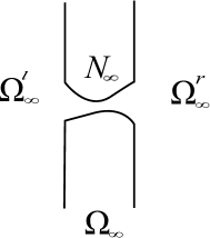
Figure 6. The limiting set $\Omega_{\infty}$.

We are now in a position to state the main result of this subsection.

Theorem 4.3 (Asymptotic behavior in the normal neck regime).

Assume (4.3) and let $(u_{\varepsilon})$ be a family of critical points as in Definition 3.1. Set

$$v_{\varepsilon}(x,y):=|\ln\varepsilon|(u_{\varepsilon}(\varepsilon x,\varepsilon y)-u_{\varepsilon}(0,0)).$$ (4.4)

Then, for every $p\geq 1$ we have $v_{\varepsilon}\to v$ in $W^{2,p}_{loc}(\Omega_{\infty})$ as $\varepsilon\to 0^{+}$, where $v$ is the unique solution to the following problem:

$$\begin{cases}\Delta v=0&\text{in $\Omega_{\infty}$,}\vspace{4pt}\\ \partial_{\nu}v=0&\text{on $\partial\Omega_{\infty}$,}\vspace{4pt}\\ \displaystyle\frac{v(x,y)}{\ln|(x,y)|}\to{\beta-\alpha\over 2}&\text{as $|(x,y)|\to+\infty$ with $x>1$,}\vspace{4pt}\\ \displaystyle\frac{v(x,y)}{\ln|(x,y)|}\to{\alpha-\beta\over 2}&\text{as $|(x,y)|\to+\infty$ with $x<1$,}\vspace{4pt}\\ v(0,0)=0\,.\end{cases}$$ (4.5)

Moreover, $u_{\varepsilon}(0,0)\to{\alpha+\beta\over 2}$ and $\nabla v_{\varepsilon}\chi_{\frac{1}{\varepsilon}\Omega_{\varepsilon}}\to\nabla v\chi_{\Omega_{\infty}}$ in $L^{2}_{loc}(\mathbb{R}^{2};\mathbb{R}^{2})$. Finally,

$$\lim_{\varepsilon\to 0^{+}}|\ln\varepsilon|\left(F(u_{\varepsilon},\Omega_{\varepsilon})-W(\beta)|\Omega^{r}|-W(\alpha)|\Omega^{l}|\right)={\pi\over 4}(\beta-\alpha)^{2}\,.$$ (4.6)

Remark 4.4.

The theorem shows that the rescaled profiles of nearly locally constant critical points (and their energy) display a universal asymptotic behavior, which depends only on the wells $\alpha$ and $\beta$, and on the limiting shape of the rescaled necks. In particular, such a behavior is independent of $\Omega^{l}$, $\Omega^{r}$, and the specific form of the double-well potential $W$.

Proof of Theorem 4.3.

To simplify the presentation and avoid inessential technicalities throughout the proof we assume $\ell=1$ and $\delta=\varepsilon$. We also assume without loss of generality that $\alpha<\beta$. Integrating by parts, we have

$$\int_{\Omega_{\varepsilon}}|\nabla u_{\varepsilon}|^{2}=\int_{\Omega_{\varepsilon}}W^{\prime}(u_{\varepsilon})u_{\varepsilon}\to 0,$$ (4.7)

where we have used the fact that $\chi_{\Omega_{\varepsilon}}W^{\prime}(u_{\varepsilon})\to 0$ in $L^{p}$ for all $p\geq 1$, which easily follows from conditions (a) and (b) of Definition 3.1. In particular,

$$\sup_{0<\varepsilon\leq\bar{\varepsilon}}\|u_{\varepsilon}\|_{H^{1}(\Omega_{\varepsilon})}<+\infty\,.$$ (4.8)

For any fixed $0<\rho_{1}<r_{0}$, let

$$A^{r}_{\varepsilon}(\rho_{1}) :=(\varepsilon,0)+\{(x,y)\in\Omega^{r}:\rho_{1}<|(x,y)|\}\,,$$ (4.9)

$$A^{l}_{\varepsilon}(\rho_{1}) :=-(\varepsilon,0)+\{(x,y)\in\Omega^{l}:\rho_{1}<|(x,y)|\}\,.$$

Recalling (4.8) and the regularity assumptions on $\Omega^{l}$ and $\Omega^{r}$, by standard elliptic estimates we have

$$\eta^{r}_{\varepsilon}:=\|u_{\varepsilon}-\beta\|_{L^{\infty}(A^{r}_{\varepsilon}(\rho_{1}))}\to 0\,,\qquad\eta^{l}_{\varepsilon}:=\|u_{\varepsilon}-\alpha\|_{L^{\infty}(A^{l}_{\varepsilon}(\rho_{1}))}\to 0\,.$$ (4.10)

We now split the remaining part of the proof into several steps.

Step 1.(limit of $u_{\varepsilon}(0,0)$ and of the energy) Set

$$M:=\max\{\|f_{1}\|_{\infty},\|f_{2}\|_{\infty}\}+1\,$$ (4.11)

where $f_{1}$ and $f_{2}$ are the functions appearing in (2.3). Since the function $\hat{u}_{\varepsilon}(x,y):=u_{\varepsilon}(\varepsilon x,\varepsilon y)$ satisfies the Euler-Lagrange equation

$$\begin{cases}\Delta\hat{u}_{\varepsilon}=\varepsilon^{2}W^{\prime}(\hat{u}_{\varepsilon}),\\ \displaystyle{\partial\hat{u}_{\varepsilon}\over\partial n}=0,\end{cases}$$

and $\int_{B_{2M}(0,0)\cap\Omega_{\infty}}|\nabla\hat{u}_{\varepsilon}|^{2}\,dxdy\,\to 0$ by (4.7), again standard regularity results imply the existence of a constant $m$ such that

$$\hat{u}_{\varepsilon}\to m\qquad\text{locally uniformly on $B_{2M}(0,0)\cap\Omega_{\infty}$}$$ (4.12)

and

$$\hat{u}_{\varepsilon}\to m\qquad\text{ uniformly on $\partial B_{M}(1,0)\cap\Omega_{\infty}$.}$$ (4.13)

Here we have also used the fact that $(\Omega_{\varepsilon}/\varepsilon)\cap B_{2M}(0,0)=\Omega_{\infty}\cap B_{2M}(0,0)$ for $\varepsilon$ small enough (see Assumption (O3) in Section 2). We claim that

$$m=\frac{\alpha+\beta}{2}\,.$$ (4.14)

To this aim, recall that for any given $\gamma\in(0,1)$, it is possible to construct a sequence of functions $\xi_{\varepsilon}$ such that $\|\xi_{\varepsilon}-u_{\varepsilon}\|_{L^{1}(\Omega_{\varepsilon})}\to 0$ and

$$\lim_{\varepsilon\to 0^{+}}|\ln\varepsilon|\left(F(\xi_{\varepsilon},\Omega_{\varepsilon})-W(\beta)|\Omega^{r}|-W(\alpha)|\Omega^{l}|\right)=\frac{(\beta-\alpha)^{2}}{4}\frac{\pi}{1-\gamma}\,,$$

see (4.2). By (3.2) and the arbitrariness of $\gamma$ we deduce that

$$\limsup_{\varepsilon\to 0^{+}}|\ln\varepsilon|\left(F(u_{\varepsilon},\Omega_{\varepsilon})-W(\beta)|\Omega^{r}|-W(\alpha)|\Omega^{l}|\right)\leq{\pi\over{4}}(\beta-\alpha)^{2}\,.$$ (4.15)

Recall now that due to (4.13) for any given $\eta>0$ and $\varepsilon$ sufficiently small we have

$$m-\eta\leq u_{\varepsilon}\leq m+\eta\qquad\text{on $\{(x,y):\,|(x-\varepsilon,y)|=M\varepsilon\,,x>\varepsilon\}$}.$$ (4.16)

Moreover, by (4.10),

$$\beta-\eta_{\varepsilon}^{r}\leq u_{\varepsilon}\leq\beta+\eta_{\varepsilon}^{r}\qquad\text{on $\{(x,y):\,|(x-\varepsilon,y)|=\rho_{1}\,,x>\varepsilon\}$.}$$

Assume now that $m<\beta$ so that for $\eta$ and $\varepsilon$ sufficiently small we also have $m+\eta<\beta-\eta_{\varepsilon}^{r}$. Then, we may estimate

$$\int_{\{M\varepsilon<|(x-\varepsilon,y)|<\rho_{1},\,x>\varepsilon\}}|\nabla u_{\varepsilon}|^{2}dxdy$$

$$\geq\min\left\{\int_{\{M\varepsilon<|(x-\varepsilon,y)|<\rho_{1},\,x>\varepsilon\}}\!\!\!|\nabla u|^{2}dxdy:\,u\leq m+\eta\text{ on }\partial B_{M\varepsilon}(\varepsilon,0)\cap\{x>\varepsilon\}\,,\right.$$

$$\left.\vphantom{\int}\qquad\qquad\qquad\qquad\quad u\geq\beta-\eta^{r}_{\varepsilon}\text{ on }\partial B_{\rho_{1}}(\varepsilon,0)\cap\{x>\varepsilon\}\right\}$$

$$=\min\left\{\int_{\{M\varepsilon<|(x-\varepsilon,y)|<\rho_{1},\,x>\varepsilon\}}\!\!\!|\nabla u|^{2}dxdy:\,u=m+\eta\text{ on }\partial B_{M\varepsilon}(\varepsilon,0)\cap\{x>\varepsilon\}\,,\right.$$

$$\left.\vphantom{\int}\qquad\qquad\qquad\qquad\quad u=\beta-\eta^{r}_{\varepsilon}\text{ on }\partial B_{\rho_{1}}(\varepsilon,0)\cap\{x>\varepsilon\}\right\}\,,$$ (4.17)

where the last equality easily follows by a standard truncation argument, recalling that $m+\eta<\beta-\eta_{\varepsilon}^{r}$. The unique minimizer of the last minimization problem is given by

$$\tilde{u}_{\varepsilon}(x,y)=m+\eta+\frac{\beta-\eta^{r}_{\varepsilon}-m-\eta}{\ln\frac{\rho_{1}}{M\varepsilon}}\ln\frac{|(x-\varepsilon,y)|}{M\varepsilon}\,.$$

The explicit computation of its Dirichlet energy, (4.17), and the arbitrariness of $\eta$ yield

$$\liminf_{\varepsilon\to 0}\frac{|\ln\varepsilon|}{2}\int_{\{M\varepsilon<|(x-\varepsilon,y)|<\rho_{1},\,x>\varepsilon\}}|\nabla u_{\varepsilon}|^{2}dxdy\geq\frac{\pi(\beta-m)^{2}}{2}\,.$$

The same inequality is trivial when $m=\beta$ and can be proven similarly when $m>\beta$, using the fact that for $\eta$ and $\varepsilon$ sufficiently small $m-\eta>\beta+\eta_{\varepsilon}^{r}$. By an analogous argument we also have

$$\liminf_{\varepsilon\to 0}\frac{|\ln\varepsilon|}{2}\int_{\{M\varepsilon<|(x+\varepsilon,y)|<\rho_{1},\,x<-\varepsilon\}}|\nabla u_{\varepsilon}|^{2}dxdy\geq\frac{\pi(\alpha-m)^{2}}{2}\,.$$

Collecting the two inequalities, we get

$$\liminf_{\varepsilon\to 0}\frac{|\ln\varepsilon|}{2}\int_{\Omega_{\varepsilon}}|\nabla u_{\varepsilon}|^{2}dxdy\geq\frac{\pi(\beta-m)^{2}}{2}+\frac{\pi(\alpha-m)^{2}}{2}\,.$$ (4.18)

We now claim that

$$\liminf_{\varepsilon\to 0^{+}}|\ln\varepsilon|\left(\int_{\Omega_{\varepsilon}}W(u_{\varepsilon})\,dxdy-W(\beta)|\Omega^{r}|-W(\alpha)|\Omega^{l}|\right)\geq 0\,.$$ (4.19)

To this aim, choose $\tau>0$ so small that that

$$W(t)\geq W(\alpha)\quad\text{for all $t\in(\alpha-\tau,\alpha+\tau)$,}\qquad W(t)\geq W(\beta)\quad\text{for all $t\in(\beta-\tau,\beta+\tau)$.}$$ (4.20)

This is possible thanks to condition (b) of Definition 3.1.

Recalling (4.16) (with $\eta=1$) and (4.10), we can apply Lemma 4.2 with $\rho_{0}:=M\varepsilon$, $a_{-}:=m-1$, $b_{-}:=\beta-\eta_{\varepsilon}^{r}$, and

$$d:=\max_{|t|\leq\sup_{\varepsilon}\|u_{\varepsilon}\|_{\infty}}|W^{\prime}(t)|$$

to deduce that

$$u_{\varepsilon}(x,y)\geq u^{-}_{\varepsilon}(x,y):=u^{-}(x-\varepsilon,y)\qquad\text{for $(x,y)\in\{M\varepsilon\leq|(x-\varepsilon,y)|\leq\rho_{1},\,x>\varepsilon\}$}\,,$$ (4.21)

where

$$u^{-}(x,y):=\frac{d|(x,y)|^{2}}{4}+\frac{\left(\beta-\eta_{\varepsilon}^{r}-m+1-\frac{d}{4}(\rho_{1}^{2}-M^{2}\varepsilon^{2})\right)}{\ln\frac{\rho_{1}}{M\varepsilon}}\ln\frac{|(x,y)|}{M\varepsilon}+m-1-\frac{d}{4}M^{2}\varepsilon^{2}\,.$$

Fix $\gamma\in(0,1)$ and note that

$$u_{\varepsilon}^{-}\geq\begin{cases}\displaystyle(\beta-\eta_{\varepsilon}^{r}-m+1)\frac{\ln\frac{\varepsilon^{\gamma}}{M\varepsilon}}{\ln\frac{\rho_{1}}{M\varepsilon}}-\frac{d}{2}\rho_{1}^{2}+m-1&\text{if $\beta-\eta_{\varepsilon}^{r}-m+1\geq 0$}\vspace{5pt}\\ \displaystyle\vphantom{\int}\beta-\eta_{\varepsilon}^{r}-\frac{d}{2}\rho_{1}^{2}&\text{otherwise}\end{cases}$$

on the set $\{\varepsilon^{\gamma}\leq|(x-\varepsilon,y)|\leq\rho_{1}\}$, provided that $\varepsilon$ is sufficiently small. By taking $\gamma$, $\rho_{1}$, and $\varepsilon$ small enough and recalling (4.10) and (4.21), we may conclude that

$$u_{\varepsilon}\geq u_{\varepsilon}^{-}\geq\beta-\tau\qquad\text{on $\{\varepsilon^{\gamma}\leq|(x-\varepsilon,y)|\leq\rho_{1}\}$.}$$

Using now the upper bound $u_{\varepsilon}^{+}:=u^{+}(\cdot-\varepsilon,\cdot)$ provided by Lemma 4.2 with $a_{+}:=m+1$, $b_{+}:=\beta+\eta_{\varepsilon}^{r}$ and $\rho_{0}=M\varepsilon$, and $d$ as before (and taking $\gamma$ and $\rho_{1}$ smaller, if needed), we can prove similarly that

$$u_{\varepsilon}\leq u_{\varepsilon}^{+}\leq\beta+\tau\qquad\text{on $\{\varepsilon^{\gamma}\leq|(x-\varepsilon,y)|\leq\rho_{1}\}$.}$$

Taking into account also (4.10), we therefore conclude that for $\varepsilon$ small enough

$$\beta-\tau\leq u_{\varepsilon}\leq\beta+\tau\qquad\text{on $A_{\varepsilon}^{r}(\varepsilon^{\gamma})$,}$$ (4.22)

where $A_{\varepsilon}^{r}(\varepsilon^{\gamma})$ is the set defined in (4.9) (with $\rho_{1}$ replaced by $\varepsilon^{\gamma}$). Clearly, the same argument shows also that (upon possible modification of $\gamma$ and $\rho_{1}$, if necessary)

$$\alpha-\tau\leq u_{\varepsilon}\leq\alpha+\tau\qquad\text{on $A_{\varepsilon}^{l}(\varepsilon^{\gamma})$}$$ (4.23)

for all $\varepsilon$ sufficiently small. Combining (4.20), (4.22), and (4.23), we obtain

$$\int_{\Omega_{\varepsilon}}W(u_{\varepsilon})\,dxdy =\int_{A_{\varepsilon}^{l}(\varepsilon^{\gamma})}W(u_{\varepsilon})\,dxdy+\int_{A_{\varepsilon}^{r}(\varepsilon^{\gamma})}W(u_{\varepsilon})\,dxdy+\int_{\Omega_{\varepsilon}\setminus\left(A_{\varepsilon}^{l}(\varepsilon^{\gamma})\cup A_{\varepsilon}^{r}(\varepsilon^{\gamma})\right)}W(u_{\varepsilon})\,dxdy$$

$$\geq W(\alpha)|\Omega^{l}|+W(\beta)|\Omega^{r}|-C\varepsilon^{2\gamma}\,,$$

for some constant $C>0$ independent of $\varepsilon$. Note that we have also used the fact that the measure of $\Omega_{\varepsilon}\setminus\left(A_{\varepsilon}^{l}(\varepsilon^{\gamma})\cup A_{\varepsilon}^{r}(\varepsilon^{\gamma})\right)$ is of order $\varepsilon^{2\gamma}$ together with the uniform $L^{\infty}$ bound on $W(u_{\varepsilon})$. From the above inequality we easily infer (4.19).

Combining (4.15), (4.18), and (4.19) we obtain

$$\liminf_{\varepsilon\to 0^{+}}|\ln\varepsilon| \left(F(u_{\varepsilon},\Omega_{\varepsilon})-W(\beta)|\Omega^{r}|-W(\alpha)|\Omega^{l}|\right)\geq\frac{\pi(\beta-m)^{2}}{2}+\frac{\pi(\alpha-m)^{2}}{2}$$

$$\geq{\pi\over{4}}(\beta-\alpha)^{2}\geq\limsup_{\varepsilon\to 0^{+}}|\ln\varepsilon|\left(F(u_{\varepsilon},\Omega_{\varepsilon})-W(\beta)|\Omega^{r}|-W(\alpha)|\Omega^{l}|\right)\,.$$

Hence, in particular,

$$\frac{\pi(\beta-m)^{2}}{2}+\frac{\pi(\alpha-m)^{2}}{2}={\pi\over{4}}(\beta-\alpha)^{2}\,,$$

which implies (4.14) and (4.6).

Step 2. (localization estimate for the energy) Let

$$c_{\varepsilon}:=\int_{\Omega_{\varepsilon}\cap B_{2M\varepsilon}(0,0)}|\nabla u_{\varepsilon}|^{2}\,dxdy.$$ (4.24)

We claim that there exist positive constants $C_{1}$ and $C_{2}$ independent of $\varepsilon$ such that

$${C_{1}\over|\ln\varepsilon|^{2}}\leq c_{\varepsilon}\leq{C_{2}\over|\ln\varepsilon|^{2}}.$$ (4.25)

We argue by contradiction assuming that, up to a subsequence, either

$$c_{\varepsilon}|\ln\varepsilon|^{2}\to\infty\quad\text{ as $\varepsilon\to 0$}$$ (4.26)

or

$$c_{\varepsilon}|\ln\varepsilon|^{2}\to 0\quad\text{ as $\varepsilon\to 0$.}$$ (4.27)

We can define for $(x,y)\in\Omega_{\varepsilon}/\varepsilon$

$$w_{\varepsilon}(x,y)={1\over\sqrt{c_{\varepsilon}}}\left(u_{\varepsilon}(\varepsilon x,\varepsilon y)-\bar{u}_{\varepsilon}\right),$$

where $\bar{u}_{\varepsilon}:=-\kern-8.96268pt\int_{B_{M\varepsilon}(0,0)\cap\Omega_{\varepsilon}}u_{\varepsilon}\,dxdy\,$. Notice that for small $\varepsilon$ we have

$$\int_{\Omega_{\infty}\cap B_{2M}(0,0)}|\nabla w_{\varepsilon}|^{2}\,dxdy=1\,.$$ (4.28)

Here we used also that fact that $\Omega_{\infty}\cap B_{2M}(0,0)=\frac{1}{\varepsilon}\Omega_{\varepsilon}\cap B_{2M}(0,0)$ for $\varepsilon$ small enough. By compactness and standard elliptic estimates, we may thus assume that, up to subsequences,

$$w_{\varepsilon}\to w_{0}\quad\text{in }W^{2,p}_{loc}({\Omega}_{\infty}\cap B_{2M}(0,0))\quad\text{and}\quad\sup_{\varepsilon}\|w_{\varepsilon}\|_{L^{\infty}({\Omega}_{\infty}\cap B_{r}(0,0))}<+\infty\text{ for all $0<r<2M$.}$$ (4.29)

Moreover the convergence is uniform away from the corner points of $\Omega_{\infty}\cap B_{M}(1,0)$, so that in particular we have $w_{\varepsilon}\to w_{0}$ uniformly on $\partial B_{M}(1,0)\cap\{x>1\}$. Set $m_{0}:=\min_{\partial B_{M}(1,0)\cap\{x>1\}}w_{0}-1$ and $M_{0}:=\max_{\partial B_{M}(1,0)\cap\{x>1\}}w_{0}+1$. Thus, for $\varepsilon$ small enough we have

$$m_{0}\leq w_{\varepsilon}\leq M_{0}\qquad\text{on }\partial B_{M}(1,0)\cap\{x>1\}$$

or, equivalently,

$$m_{0}\sqrt{c_{\varepsilon}}+\bar{u}_{\varepsilon}\leq u_{\varepsilon}\leq M_{0}\sqrt{c_{\varepsilon}}+\bar{u}_{\varepsilon}\qquad\text{on }\partial B_{M\varepsilon}(\varepsilon,0)\cap\{x>\varepsilon\}\,.$$

We can now apply Lemma 4.2 with $\rho_{0}:=M\varepsilon$, $a_{-}:=m_{0}\sqrt{c_{\varepsilon}}+\bar{u}_{\varepsilon}$, $a_{+}:=M_{0}\sqrt{c_{\varepsilon}}+\bar{u}_{\varepsilon}$, $b_{-}:=\beta-\eta_{\varepsilon}^{r}$, $b_{+}:=\beta+\eta_{\varepsilon}^{r}$ and

$$d:=\max_{|t|\leq\sup_{\varepsilon}\|u_{\varepsilon}\|_{\infty}}|W^{\prime}(t)|$$ (4.30)

to deduce that

$$u^{-}_{\varepsilon}(x,y):=u^{-}(x-\varepsilon,y)\leq u_{\varepsilon}(x,y)\leq u^{+}_{\varepsilon}(x,y):=u^{+}(x-\varepsilon,y)\\ \text{for $(x,y)\in\{M\varepsilon\leq|(x-\varepsilon,y)|\leq\rho_{1},\,x>\varepsilon\}$}\,,$$ (4.31)

where

$$u^{-}(x,y):=\frac{d|(x,y)|^{2}}{4}+\frac{\left(\beta-\eta_{\varepsilon}^{r}-m_{0}\sqrt{c_{\varepsilon}}-\bar{u}_{\varepsilon}-\frac{d}{4}(\rho_{1}^{2}-M^{2}\varepsilon^{2})\right)}{\ln\frac{\rho_{1}}{M\varepsilon}}\ln\frac{|(x,y)|}{M\varepsilon}\\ +m_{0}\sqrt{c_{\varepsilon}}+\bar{u}_{\varepsilon}-\frac{d}{4}M^{2}\varepsilon^{2}$$

and

$$u^{+}(x,y):=-\frac{d|(x,y)|^{2}}{4}+\frac{\left(\beta+\eta_{\varepsilon}^{r}-M_{0}\sqrt{c_{\varepsilon}}-\bar{u}_{\varepsilon}+\frac{d}{4}(\rho_{1}^{2}-M^{2}\varepsilon^{2})\right)}{\ln\frac{\rho_{1}}{M\varepsilon}}\ln\frac{|(x,y)|}{M\varepsilon}\\ +M_{0}\sqrt{c_{\varepsilon}}+\bar{u}_{\varepsilon}+\frac{d}{4}M^{2}\varepsilon^{2}\,.$$

Assume now that (4.26) holds. Then, it is straightforward to check that

$$\frac{u^{-}_{\varepsilon}(\varepsilon\cdot,\varepsilon\cdot)-\bar{u}_{\varepsilon}}{\sqrt{c_{\varepsilon}}}\to m_{0}\,,\quad\frac{u^{+}_{\varepsilon}(\varepsilon\cdot,\varepsilon\cdot)-\bar{u}_{\varepsilon}}{\sqrt{c_{\varepsilon}}}\to M_{0}\quad\text{locally uniformly in $\{x>1\}\setminus B_{M}(1,0)$.}$$

Since

$$\frac{u^{-}_{\varepsilon}(\varepsilon\cdot,\varepsilon\cdot)-\bar{u}_{\varepsilon}}{\sqrt{c_{\varepsilon}}}\leq w_{\varepsilon}\leq\frac{u^{+}_{\varepsilon}(\varepsilon\cdot,\varepsilon\cdot)-\bar{u}_{\varepsilon}}{\sqrt{c_{\varepsilon}}}$$

and recalling (4.29), we deduce that $w_{\varepsilon}$ are locally uniformly bounded in $\Omega_{\infty}\cap\{x>0\}$. A completely analogous argument shows that the same locally uniform bounds hold in $\Omega_{\infty}\cap\{x<0\}$. Therefore, by standard arguments (see for instance [16, Proposition 6.2]) we can conclude that, up to a subsequence, $w_{\varepsilon}\to w_{0}$ in $W^{2,p}_{loc}(\Omega_{\infty})$ for all $p>2$, where $w_{0}$ is a bounded harmonic function in $\Omega_{\infty}$ satisfying homogeneous Neumann boundary conditions on $\partial\Omega_{\infty}$. Using the Riemann mapping theorem we can find a conformal mapping $\Psi$ from the infinite strip $\mathcal{R}:=(-1,1)\times\mathbb{R}$ onto $\Omega_{\infty}$. Thus, $w_{0}\circ\Psi$ is bounded and harmonic in $\mathcal{R}$ and satisfies a homogeneous Neumann condition on $\partial\mathcal{R}$. By reflecting $w_{0}\circ\Psi$ infinitely many times, we obtain a bounded entire harmonic function, which then must be constant by Liouville theorem. Since we also have $\nabla w_{\varepsilon}\chi_{\frac{\Omega_{\varepsilon}}{\varepsilon}}\to\nabla w_{0}\chi_{\Omega_{\infty}}$ in $L^{2}_{loc}(\mathbb{R}^{2};\mathbb{R}^{2})$ (see again [16, Proposition 6.2]), it follows, in particular,

$$\int_{\Omega_{\infty}\cap B_{2M}(0,0)}|\nabla w_{\varepsilon}|^{2}\,dxdy=\int_{\frac{\Omega_{\varepsilon}}{\varepsilon}\cap B_{2M}(0,0)}|\nabla w_{\varepsilon}|^{2}\,dxdy\to\int_{\Omega_{\infty}\cap B_{2M}(0,0)}|\nabla w_{0}|^{2}\,dxdy=0\,,$$

a contradiction to (4.28).

We now assume that (4.27) holds. Using also the fact that

$$\bar{u}_{\varepsilon}\to\frac{\alpha+\beta}{2}\,,$$ (4.32)

which follows from (4.12) and (4.14), one can check in this case that

$$w_{\varepsilon}\geq\frac{u^{-}_{\varepsilon}(\varepsilon x,\varepsilon y)-\bar{u}_{\varepsilon}}{\sqrt{c_{\varepsilon}}}\to+\infty$$

for all $(x,y)\in\{x>1\}\setminus B_{M}(1,0)$. This, in turn, gives a contradiction to (4.29) and concludes the proof of (4.25).

Step 3. (conclusion) Set now

$$\widetilde{w}_{\varepsilon}(x,y):=|\ln\varepsilon|(u_{\varepsilon}(\varepsilon x,\varepsilon y)-\bar{u}_{\varepsilon})\,.$$

Using (4.25), it follows that

$$\int_{\Omega_{\infty}\cap B_{2M}(0,0)}|\nabla\widetilde{w}_{\varepsilon}|^{2}\,dxdy\leq C$$

for some constant $C$ independent of $\varepsilon$. Thus, arguing exactly as before, we may deduce the existence of $\widetilde{w}_{0}$ such that, up to subsequences,

$$\widetilde{w}_{\varepsilon}\to\widetilde{w}_{0}\quad\text{in }W^{2,p}_{loc}({\Omega}_{\infty}\cap B_{2M}(0,0))\text{ and }\sup_{\varepsilon}\|\widetilde{w}_{\varepsilon}\|_{L^{\infty}({\Omega}_{\infty}\cap B_{r}(0,0))}<+\infty\text{ for $0<r<2M$.}$$ (4.33)

Moreover, again exactly as before, we may also show that

$$|\ln\varepsilon|(\widetilde{u}^{-}_{\varepsilon}(\varepsilon\cdot,\varepsilon\cdot)-\bar{u}_{\varepsilon})\leq\widetilde{w}_{\varepsilon}\leq|\ln\varepsilon|(\widetilde{u}^{+}_{\varepsilon}(\varepsilon\cdot,\varepsilon\cdot)-\bar{u}_{\varepsilon})\,,$$

where $\widetilde{u}^{-}_{\varepsilon}$ and $\widetilde{u}^{+}_{\varepsilon}$ are defined as $u^{-}_{\varepsilon}$ and $u^{+}_{\varepsilon}$, respectively, with $c_{\varepsilon}$, $m_{0}$, and $M_{0}$ replaced by $\frac{1}{|\ln\varepsilon|^{2}}$, $\widetilde{m}_{0}:=\min_{\partial B_{M}(1,0)\cap\{x>1\}}\widetilde{w}_{0}-1$, and $\widetilde{M}_{0}:=\max_{\partial B_{M}(1,0)\cap\{x>1\}}\widetilde{w}_{0}+1$, respectively. By a straightforward computation, taking into account (4.32), we have that

$$\begin{array}[]{c}|\ln\varepsilon|(\widetilde{u}^{-}_{\varepsilon}(\varepsilon x,\varepsilon y)-\bar{u}_{\varepsilon})\to\displaystyle\widetilde{m}_{0}+\frac{\beta-\alpha}{2}\ln\frac{|(x-1,y)|}{M}\,,\vspace{5pt}\\ |\ln\varepsilon|(\widetilde{u}^{+}_{\varepsilon}(\varepsilon x,\varepsilon y)-\bar{u}_{\varepsilon})\to\displaystyle\widetilde{M}_{0}+\frac{\beta-\alpha}{2}\ln\frac{|(x-1,y)|}{M}\end{array}$$ (4.34)

for all $(x,y)\in\{x>1\}\setminus B_{M}(1,0)$. The convergence is in fact uniform on the bounded subsets of $\{x>1\}\setminus B_{M}(1,0)$. Recalling that $\widetilde{w}_{\varepsilon}$ satisfies

$$\begin{cases}\Delta\widetilde{w}_{\varepsilon}=|\ln\varepsilon|\varepsilon^{2}W^{\prime}(u_{\varepsilon})&\text{in $\frac{\Omega_{\varepsilon}}{\varepsilon}$,}\\ \displaystyle\frac{\partial\widetilde{w}_{\varepsilon}}{\partial\nu}=0&\text{on $\frac{\partial\Omega_{\varepsilon}}{\varepsilon}$,}\end{cases}$$

using (4.33), (4.34), and the corresponding bounds in $\{x<-1\}\setminus B_{M}(-1,0)$, by [16, Proposition 6.2] we can deduce that, up to subsequences,

$$\widetilde{w}_{\varepsilon}\to\widetilde{w}_{0}\quad\text{in $W^{2,p}_{loc}(\Omega_{\infty})$,}$$ (4.35)

with $\widetilde{w}_{0}$ solving

$$\begin{cases}\Delta\widetilde{w}_{0}=0&\text{in $\Omega_{\infty}$,}\vspace{4pt}\\ \displaystyle\frac{\partial\widetilde{w}_{0}}{\partial\nu}=0&\text{on $\partial\Omega_{\infty}$,}\vspace{4pt}\\ \displaystyle\frac{\widetilde{w}_{0}(x,y)}{\ln|(x,y)|}\to{\beta-\alpha\over 2}&\text{as $|(x,y)|\to+\infty$ with $x>1$,}\vspace{4pt}\\ \displaystyle\frac{\widetilde{w}_{0}(x,y)}{\ln|(x,y)|}\to{\alpha-\beta\over 2}&\text{as $|(x,y)|\to+\infty$ with $x<-1$.}\end{cases}$$ (4.36)

Next we claim that

$$|\ln\varepsilon||\bar{u}_{\varepsilon}-u_{\varepsilon}(0,0)|\leq C$$ (4.37)

for some constant $C$ independent of $\varepsilon$. To this aim, fix $0<\rho_{0}<M$ so small that $B_{\rho_{0}}(0,0)\subset\subset\Omega_{\infty}$ and define $a_{\varepsilon}:=-\kern-8.96268pt\int_{B_{\rho_{0}}(0,0)}u_{\varepsilon}(\varepsilon x,\varepsilon y)\,dxdy$. Notice that

$$|\bar{u}_{\varepsilon}-a_{\varepsilon}| \leq-\kern-10.66977pt\int_{B_{M}(0,0)\cap\Omega_{\infty}}|u_{\varepsilon}(\varepsilon x,\varepsilon y)-a_{\varepsilon}|\,dxdy$$

$$\leq C\|u_{\varepsilon}(\varepsilon\cdot,\varepsilon\cdot)-a_{\varepsilon}\|_{L^{2}(B_{M}(0,0)\cap\Omega_{\infty})}\leq\frac{C}{|\ln\varepsilon|}\,,$$ (4.38)

where the least inequality follows from the Poincaré-Wirtinger inequality, (4.24), and (4.25). Observe now that by the Sobolev Embedding Theorem and standard elliptic estimates, we have for any $p>2$

$$\|\nabla u_{\varepsilon}(\varepsilon\cdot,\varepsilon\cdot)\|_{C^{0}(B_{\rho_{0}}(0,0))} \leq C\|u_{\varepsilon}(\varepsilon\cdot,\varepsilon\cdot)-\bar{u}_{\varepsilon}\|_{W^{2,p}(B_{\rho_{0}}(0,0))}$$

$$\leq C(\|\varepsilon^{2}W^{\prime}(u_{\varepsilon})\|_{L^{p}(B_{M}(0,0)\cap\Omega_{\infty})}+\|u_{\varepsilon}(\varepsilon\cdot,\varepsilon\cdot)-\bar{u}_{\varepsilon}\|_{H^{1}(B_{M}(0,0)\cap\Omega_{\infty})})\leq\frac{C}{|\ln\varepsilon|}\,,$$

where the last inequality follows again from (4.24) and (4.25). From the above inequality, it immediately follows that

$$|a_{\varepsilon}-u_{\varepsilon}(0,0)|\leq\frac{C}{|\ln\varepsilon|}\,,$$

which together with (4.38) yields (4.37).

We are now ready to conclude. Indeed, by (4.35) and (4.37), we have that, up to a further subsequence, the functions $v_{\varepsilon}$ defined in (4.4) converge to $v$ in $W^{2,p}_{loc}(\Omega_{\infty})$ for every $p\geq 1$, where $v$ solves (4.5). Since the solution to this problem is unique, as shown in Step 5 of the proof of [16, Theorem 3.1], the convergence holds for the full sequence. Finally, the fact that $u_{\varepsilon}(0,0)\to\frac{\alpha+\beta}{2}$ follows from (4.32) and (4.37).

∎

4.2. The thick neck regime

In this subsection we state the result concerning the asymptotic behavior of admissible families of critical point in the so-called thick neck regime. We omit the proof since it is similar (and in fact easier) to that of Theorem 4.3. We define

$$y_{i}=\min\{\,f_{i}(x),\,x\in[-1,1]\,\}\quad\text{for }i=1,2\,.$$

Using assumptions on $f_{i}(x)$ it is clear that $y_{i}>0$ for $i=1,2$.

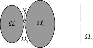
Figure 7. The limiting set $\Omega^{+}_{\infty}$.

Theorem 4.5.

Assume that

$$\lim_{\varepsilon\to 0^{+}}\frac{\delta}{\varepsilon}=+\infty\,.$$

Let $(u_{\varepsilon})$ be a family of critical points as in Definition 3.1 and set

$$v_{\varepsilon}(x,y):=|{\ln\delta}|(u_{\varepsilon}(\delta x,\delta y)-u_{\varepsilon}(0,0))$$

and $\Omega_{\infty}:=\mathbb{R}^{2}\setminus\{(0,y):\,y\geq y_{1}\text{ or }y\leq-y_{2}\}$. Then, for every $p\geq 1$ we have $v_{\varepsilon}\to v$ in $W^{2,p}_{loc}(\Omega_{\infty})$, where $v$ is the unique solution to the following problem:

$$\begin{cases}\Delta v=0&\text{in $\Omega_{\infty}$,}\vspace{4pt}\\ \partial_{\nu}v=0&\text{on $\partial\Omega_{\infty}$,}\vspace{4pt}\\ \displaystyle\frac{v(x,y)}{\ln|(x,y)|}\to\frac{\beta-\alpha}{2}&\text{as $|(x,y)|\to+\infty$ with $x>0$,}\vspace{4pt}\\ \displaystyle\frac{v(x,y)}{\ln|(x,y)|}\to\frac{\alpha-\beta}{2}&\text{as $|(x,y)|\to+\infty$ with $x<0$,}\vspace{4pt}\\ v(0,0)=0\,.\end{cases}$$

Moreover, $u_{\varepsilon}(0,0)\to\frac{\alpha+\beta}{2}$ and $\nabla v_{\varepsilon}\chi_{\frac{1}{\delta}\Omega_{\varepsilon}}\to\nabla v\chi_{\Omega_{\infty}}$ in $L^{2}_{loc}(\mathbb{R}^{2};\mathbb{R}^{2})$. Finally,

$$\lim_{\varepsilon\to 0^{+}}|\ln\delta|(F(u_{\varepsilon},\Omega_{\varepsilon})-W(\beta)|\Omega^{r}|-W(\alpha)|\Omega^{l}|)=\frac{\pi}{4}(\beta-\alpha)^{2}\,.$$

4.3. The thin neck regime

We now consider the critical thin neck regime. To simplify the presentation, we additionally assume that $f_{1}$ and $f_{2}$ are constant in a neighborhood of the points $-1$ and $1$. Precisely, there exists $\eta_{0}>0$ such that

$$f^{\prime}_{i}(x)=0\quad\text{ for }x\in(1-\eta_{0},1)\cup(-1,-1+\eta_{0})\,,\quad i=1,2\,.$$ (4.39)

As it will be clear from the proof of the main result, the above assumption allows to avoid some technicalities in the construction of suitable lower and upper bounds and to present the main ideas in a more transparent way. It could be removed by using the lower and upper bounds constructed in [16], see Remark 4.10 below.

In order to state the next result, we set

$$m_{{}_{f_{1}f_{2}}}:=\int_{-1}^{1}\frac{1}{f_{1}+f_{2}}\,dx\,.$$ (4.40)

Figure 8. The limiting set $\Omega^{+}_{\infty}$.

Theorem 4.6 (Critical thin neck).

Assume that

$$\lim_{\varepsilon\to 0^{+}}\frac{\delta|\ln\delta|}{\varepsilon}=\ell\in(0,+\infty)\,.$$ (4.41)

Let $\{u_{\varepsilon}\}$ be the family of critical points as in Definition 3.1. Then the following statements hold true.

1. Let $\{v_{\varepsilon}\}$ be the family of rescaled profiles defined by

   $$v_{\varepsilon}(x,y):=u_{\varepsilon}(\varepsilon x,\delta y)\,.$$ (4.42)

   Then $v_{\varepsilon}\to v$ in $H^{1}(N)$, where $v(x,y):=\hat{v}(x)$ with $\hat{v}$ being the unique solution to the one-dimensional problem

   $$\qquad\qquad\min\left\{\int_{-1}^{1}\frac{f_{1}+f_{2}}{2}(\theta^{\prime})^{2}\,dx:\,\theta\in H^{1}(-1,1),\,\right.\\ \left.\theta(\pm 1)=\frac{\alpha+\beta}{2}\pm\frac{\pi\,m_{{}_{f_{1}f_{2}}}(\beta-\alpha)}{2(\pi\,m_{{}_{f_{1}f_{2}}}+2\ell)}\right\}\,,$$ (4.43)

   where $m_{{}_{f_{1}f_{2}}}$ is the constant defined in (4.40). Moreover,

   $$\lim_{\varepsilon\to 0^{+}}|\ln\delta|F(u_{\varepsilon},N_{\varepsilon})=\frac{\ell\pi^{2}\,m_{{}_{f_{1}f_{2}}}(\beta-\alpha)^{2}}{2\left(\pi\,m_{{}_{f_{1}f_{2}}}+2\ell\right)^{2}}\,.$$ (4.44)

2. Define

   $$w_{\varepsilon}^{\pm}(x,y):=|\ln\delta|(u_{\varepsilon}(\delta x\pm\varepsilon,\delta y)-u_{\varepsilon}(\pm\varepsilon,0))\quad\text{for }(x,y)\in\widetilde{\Omega}_{\varepsilon}^{\pm}:=\tfrac{\Omega^{\pm}_{\varepsilon}+(\mp\varepsilon,0)}{\delta}\,.$$ (4.45)

   Then,

   $$u_{\varepsilon}(\pm\varepsilon,0)\to\frac{\alpha+\beta}{2}\pm\frac{\pi\,m_{{}_{f_{1}f_{2}}}(\beta-\alpha)}{2(\pi\,m_{{}_{f_{1}f_{2}}}+2\ell)}\quad\text{as $\varepsilon\to 0^{+}$}$$ (4.46)

   and the functions $w_{\varepsilon}^{\pm}$ converge in $W^{2,p}_{loc}(\Omega^{\pm}_{\infty})$ for every $p\geq 1$ to the unique solution $w^{\pm}$ of the problem

   $$\begin{cases}\Delta w^{\pm}=0&\text{in $\Omega^{\pm}_{\infty}$,}\vspace{4pt}\\ \partial_{\nu}w^{\pm}=0&\text{on $\partial\Omega^{\pm}_{\infty}$, }\vspace{4pt}\\ \displaystyle\frac{w^{\pm}(x,y)}{\ln|(x,y)|}\to\pm\frac{(\beta-\alpha)\ell}{\pi\,m_{{}_{f_{1}f_{2}}}+2\ell}&\text{as $|(x,y)|\to\pm\infty$ with $\pm x>0$,}\vspace{4pt}\\ \displaystyle\frac{w^{\pm}(x,y)}{x}\to\frac{1}{(f_{1}+f_{2})(\pm 1)}\frac{(\beta-\alpha)\ell\pi}{\pi\,m_{{}_{f_{1}f_{2}}}+2\ell}&\text{uniformly in $y$ as $x\to\mp\infty$,}\vspace{4pt}\\ w^{\pm}(0,0)=0\,,\end{cases}$$ (4.47)

   where (see Figure 8)

   $$\Omega_{\infty}^{\pm}:=\left\{(x,y):\,\pm x\leq 0\,,-f_{2}(\pm 1)<y<f_{1}(\pm 1)\right\}\cup\{(x,y):\,\pm x>0\}\,.$$ (4.48)

   Moreover, $\nabla w_{\varepsilon}^{\pm}\chi_{\widetilde{\Omega}_{\varepsilon}^{\pm}}\to\nabla w^{\pm}\chi_{\Omega^{\pm}_{\infty}}$ in $L^{2}_{loc}(\mathbb{R}^{2};\mathbb{R}^{2})$.

3. We have

   $$\lim_{\varepsilon\to 0^{+}}|\ln\delta|\left(F(u_{\varepsilon},\Omega_{\varepsilon}\setminus N_{\varepsilon})-W(\beta)|\Omega^{r}|-W(\alpha)|\Omega^{l}|\right)=\frac{(\beta-\alpha)^{2}\ell^{2}\pi}{\left(\pi\,m_{{}_{f_{1}f_{2}}}+2\ell\right)^{2}}\,.$$ (4.49)

For an interpretation of the boundary data $\theta(\pm 1)$ appearing in the one-dimensional minimum problem (4.43) in terms of a suitable limiting renormalized energy see Remark 4.11 below.

Remark 4.7.

The boundary conditions appearing in problem (4.43) show that only a part of the transition occurs inside the neck. The one-dimensional limiting profile described by (4.43) is determined only by the shape of the neck itself. Note also that in (4.47) the geometry is “linearized” and the shape of the neck “weakly” affects the limiting bulk behavior only through the constant $m_{{}_{f_{1}f_{2}}}$ appearing in the conditions at infinity. We finally remark that the two conditions at infinity in (4.47) are not independent, as shown by Proposition 4.8 below.

Before starting the proof of the theorem we recall the following proposition proved in [16, Proposition 4.14].

Proposition 4.8.

Let $\alpha$, $\beta>0$ and consider the set

$$\Omega^{+}_{\infty}:=\{(x,y):\,x\leq 0,\,|y|<\tfrac{\alpha}{2}\}\cup\{(x,y):\,x>0\}\,.$$

Then, the problem

$$\begin{cases}\Delta w=0&\text{in $\Omega^{+}_{\infty}$,}\vspace{4pt}\\ \partial_{\nu}w=0&\text{on $\partial\Omega^{+}_{\infty}$,}\vspace{4pt}\\ \displaystyle\frac{w(x,y)}{\ln|(x,y)|}\to\beta&\text{as $|(x,y)|\to+\infty$ with $x>0$,}\vspace{4pt}\\ \text{$w$ grows at most linearly in $\Omega^{+}_{\infty}\cap\{x<0\}$,}\vspace{4pt}\\ w(0,0)=0\end{cases}$$ (4.50)

admits a unique solution. Moreover,

$$\frac{w(x,y)}{x}\to\frac{\pi\beta}{\alpha}\qquad\text{uniformly in $y$ as $x\to-\infty$.}$$ (4.51)

Remark 4.9.

We stress that the previous statement implies that the logarithmic behavior of $w|_{\{x>0\}}$ at infinity, cobimbined with the special one-dimensional geometry of the domain in $\{x<0\}$, uniquely determine the linear asymptotic behavior of $w|_{\{x<0\}}$.

Proof of Theorem 4.6.

We split the proof into several steps.

Step 1. (energy bounds in the neck) First of all note that the same argument used to prove (4.19), yields

$$\begin{array}[]{c}\displaystyle\liminf_{\varepsilon\to 0^{+}}|\ln\delta|\left(\int_{\Omega^{r}_{\varepsilon}}W(u_{\varepsilon})\,dxdy-W(\beta)|\Omega^{r}|\right)\geq 0\\ \text{and}\\ \displaystyle\liminf_{\varepsilon\to 0^{+}}|\ln\delta|\left(\int_{\Omega^{l}_{\varepsilon}}W(u_{\varepsilon})\,dxdy-W(\alpha)|\Omega^{l}|\right)\geq 0\,.\end{array}$$ (4.52)

Considering the function $v_{\varepsilon}$ defined in (4.42), and recalling (4.1) and using (4.52), it follows

$$\int_{N_{\varepsilon}}|\nabla u_{\varepsilon}|^{2}\,dxdy =\int_{N_{\varepsilon}}\left[\frac{1}{\varepsilon^{2}}\Bigl{|}\partial_{x}v_{\varepsilon}\Bigl{(}\frac{x}{\varepsilon},\frac{y}{\delta}\Bigr{)}\Bigr{|}^{2}+\frac{1}{\delta^{2}}\Bigl{|}\partial_{y}v_{\varepsilon}\Bigl{(}\frac{x}{\varepsilon},\frac{y}{\delta}\Bigr{)}\Bigr{|}^{2}\right]\,dxdy$$

$$=\int_{N}\left[\frac{\delta}{\varepsilon}|\partial_{x}v_{\varepsilon}(x,y)|^{2}+\frac{\varepsilon}{\delta}|\partial_{y}v_{\varepsilon}(x,y)|^{2}\right]\,dxdy\leq\frac{C}{|\ln\delta|}\,,$$ (4.53)

with $N$ defined in (2.4). Multiplying both sides of the last inequality by $\varepsilon/\delta$ and recalling (4.41), we obtain

$$\int_{N}\left[|\partial_{x}v_{\varepsilon}(x,y)|^{2}+\frac{\varepsilon^{2}}{\delta^{2}}|\partial_{y}v_{\varepsilon}(x,y)|^{2}\right]\,dxdy\leq C$$ (4.54)

for some constant $C>0$ independent of $\varepsilon$. Since $\varepsilon/\delta\to\infty$ as $\varepsilon\to 0$, by (4.54) we easily deduce that $v_{\varepsilon}$ is bounded in $H^{1}(N)$ and, up to subsequences,

$$v_{\varepsilon}\rightharpoonup v\qquad\text{weakly in $H^{1}(N)$}$$ (4.55)

for some one-dimensional $v$ of the form

$$v(x,y)=\hat{v}(x)\qquad\text{with $\hat{v}\in H^{1}(-1,1)$.}$$ (4.56)

We will show that $\hat{v}$ is independent of the subsequence and solves (4.43).

From (4.41), (4.53), (4.55), and (4.56) we have

$$\liminf_{\varepsilon\to 0}|\ln\delta|F(u_{\varepsilon},N_{\varepsilon})\geq\liminf_{\varepsilon\to 0}|\ln\delta|\frac{1}{2}\int_{N_{\varepsilon}}|\nabla u_{\varepsilon}|^{2}\,dxdy$$

$$=\liminf_{\varepsilon\to 0}\frac{1}{2}\int_{N}\left[\frac{\delta|\ln\delta|}{\varepsilon}|\partial_{x}v_{\varepsilon}(x,y)|^{2}+\frac{\varepsilon|\ln\delta|}{\delta}|\partial_{y}v_{\varepsilon}(x,y)|^{2}\right]\,dxdy$$

$$\geq\liminf_{\varepsilon\to 0}\frac{\ell}{2}\int_{N}|\nabla v_{\varepsilon}|^{2}\,dxdy\geq\frac{\ell}{2}\int_{N}|\nabla v|^{2}\,dxdy$$

$$=\frac{\ell}{2}\int_{-1}^{1}(f_{1}+f_{2})(\hat{v}^{\prime})^{2}\,dx$$

$$\geq\frac{\ell}{2}\min\left\{\int_{-1}^{1}(f_{1}+f_{2})(\theta^{\prime})^{2}\,dx:\,\theta\in H^{1}(-1,1)\,,\theta(\pm 1)=\hat{v}(\pm 1)\right\}$$

$$=\frac{\ell\left(\hat{v}(1)-\hat{v}(-1)\vphantom{\int}\right)^{2}}{2m_{{}_{f_{1}f_{2}}}}\,.$$ (4.57)

The last equality follows from the explicit computation of the minimum problem.

Step 2. (energy bounds in the bulk) Let $\bar{r}>0$ satisfy $2\bar{r}<\min_{[-1,1]}f_{i}$, $i=1,2$. Since $\hat{u}_{\varepsilon}(x,y):=u_{\varepsilon}(\delta x+\varepsilon,\delta y)$ satisfies

$$\Delta\hat{u}_{\varepsilon}=\delta^{2}W^{\prime}(\hat{u}_{\varepsilon}),\qquad\text{in $B_{2\bar{r}}(0,0)$}$$

and recalling that by (4.7), $\int_{B_{2\bar{r}}(0,0)}|\nabla\hat{u}_{\varepsilon}|^{2}\,dxdy\,\to 0$, using standard regularity theory results we conclude that there exists a constant $m$ such that

$$\hat{u}_{\varepsilon}\to m\qquad\text{uniformly on $B_{\bar{r}}(0,0)$.}$$ (4.58)

We claim that

$$m=\hat{v}(1)\,.$$ (4.59)

For this it is enough to observe that from (4.55) and (4.56) it easily follows that $v_{\varepsilon}(\cdot,y)\rightharpoonup\hat{v}$ weakly in $H^{1}(-1,1)$ for almost every $y\in(-2\bar{r},2\bar{r})$. Thus, in particular, $v_{\varepsilon}(1,y)\to\hat{v}(1)$ for almost every $y\in(-\bar{r},\bar{r})$. Since $\hat{u}_{\varepsilon}(0,y)=v_{\varepsilon}(1,y)$, the claim follows from (4.58). We can now argue exactly as in the proof of (4.18) and use (4.52) to obtain that

$$\liminf_{\varepsilon\to 0^{+}}|\ln\delta|\left(F(u_{\varepsilon},\Omega^{r}_{\varepsilon})-W(\beta)|\Omega^{r}|\right)\geq\frac{\pi(\beta-\hat{v}(1))^{2}}{2}\,.$$ (4.60)

Analogously, one can show that

$$\liminf_{\varepsilon\to 0^{+}}|\ln\delta|\left(F(u_{\varepsilon},\Omega^{l}_{\varepsilon})-W(\alpha)|\Omega^{l}|\right)\geq\frac{\pi(\alpha-\hat{v}(-1))^{2}}{2}\,.$$ (4.61)

Step 3. (asymptotic behavior in the neck and limit of the energy) By (4.57), (4.60), and (4.61) we have

$$\liminf_{\varepsilon\to 0}|\ln\delta|(F(u_{\varepsilon},\Omega_{\varepsilon})-W(\alpha)|\Omega^{l}|-W(\beta)|\Omega^{r}|)\geq\\ \frac{\ell\left(\hat{v}(1)-\hat{v}(-1)\vphantom{\int}\right)^{2}}{2m_{{}_{f_{1}f_{2}}}}+\frac{\pi(\alpha-\hat{v}(-1))^{2}}{2}+\frac{\pi(\beta-\hat{v}(1))^{2}}{2}\geq\frac{(\beta-\alpha)^{2}\pi\ell}{2(m_{{}_{f_{1}f_{2}}}\pi+2\ell)}\,.$$ (4.62)

Note that

$$\frac{\ell\left(\hat{v}(1)-\hat{v}(-1)\vphantom{\int}\right)^{2}}{2m_{{}_{f_{1}f_{2}}}}+\frac{\pi(\alpha-\hat{v}(-1))^{2}}{2}+\frac{\pi(\beta-\hat{v}(1))^{2}}{2}=\frac{(\beta-\alpha)^{2}\pi\ell}{2(m_{{}_{f_{1}f_{2}}}\pi+2\ell)}\\ \iff\hat{v}(-1)=\frac{\alpha+\beta}{2}-\frac{\pi\,m_{{}_{f_{1}f_{2}}}(\beta-\alpha)}{2(\pi\,m_{{}_{f_{1}f_{2}}}+2\ell)}\,\quad\text{ and }\quad\hat{v}(1)=\frac{\alpha+\beta}{2}+\frac{\pi\,m_{{}_{f_{1}f_{2}}}(\beta-\alpha)}{2(\pi\,m_{{}_{f_{1}f_{2}}}+2\ell)}\,,$$ (4.63)

as it easily follows by minimizing the function on the left-hand side with respect to $\hat{v}(-1)$ and $\hat{v}(1)$. On the other hand, for any fixed $\gamma\in(0,1)$ and for $M$ as in (4.11), we may consider the test functions $z_{\varepsilon}$ defined as

$$z_{\varepsilon}(x,y):=\\ \begin{cases}\frac{1}{\varepsilon}\frac{\pi(\beta-\alpha)}{m_{{}_{f_{1}f_{2}}}\pi+2\ell}\int_{-\varepsilon}^{x}\frac{1}{(f_{1}+f_{2})(\frac{s}{\varepsilon})}\,ds+\frac{\alpha+\beta}{2}-\frac{\pi\,m_{{}_{f_{1}f_{2}}}(\beta-\alpha)}{2(\pi\,m_{{}_{f_{1}f_{2}}}+2\ell)}&\text{in $N_{\varepsilon}$,}\vspace{6pt}\\ \frac{\alpha+\beta}{2}-\frac{\pi\,m_{{}_{f_{1}f_{2}}}(\beta-\alpha)}{2(\pi\,m_{{}_{f_{1}f_{2}}}+2\ell)}&\text{in $\{|(x+\varepsilon,y)|\leq M\delta,\,x<-\varepsilon\}$,}\vspace{6pt}\\ \frac{\alpha+\beta}{2}+\frac{\pi\,m_{{}_{f_{1}f_{2}}}(\beta-\alpha)}{2(\pi\,m_{{}_{f_{1}f_{2}}}+2\ell)}&\text{in $\{|(x-\varepsilon,y)|\leq M\delta,\,x>\varepsilon\}$,}\vspace{6pt}\\ \frac{\ell(\beta-\alpha)}{m_{{}_{f_{1}f_{2}}}\pi+2\ell}\frac{1}{\left|\ln M\delta^{1-\gamma}\right|}\ln\frac{|(x+\varepsilon,y)|}{\delta^{\gamma}}+\alpha&\text{in $\{M\delta<|(x+\varepsilon,y)|<\delta^{\gamma},\,x<-\varepsilon\}$,}\vspace{6pt}\\ \alpha&\text{otherwise in $\Omega^{l}_{\varepsilon}$,}\vspace{6pt}\\ -\frac{\ell(\beta-\alpha)}{m_{{}_{f_{1}f_{2}}}\pi+2\ell}\frac{1}{\left|\ln M\delta^{1-\gamma}\right|}\ln\frac{|(x-\varepsilon,y)|}{\delta^{\gamma}}+\beta&\text{in $\{M\delta<|(x-\varepsilon,y)|<\delta^{\gamma},\,x>\varepsilon\}$,}\vspace{6pt}\\ \beta&\text{otherwise in $\Omega^{r}_{\varepsilon}$.}\end{cases}$$

Taking into account the local minimality of $u_{\varepsilon}$, we have

$$\limsup_{\varepsilon\to 0}|\ln\delta| (F(u_{\varepsilon},\Omega_{\varepsilon})-W(\alpha)|\Omega^{l}|-W(\beta)|\Omega^{r}|)$$

$$\leq\limsup_{\varepsilon\to 0}|\ln\delta|(F(z_{\varepsilon},\Omega_{\varepsilon})-W(\alpha)|\Omega^{l}|-W(\beta)|\Omega^{r}|)$$

$$\leq\lim_{\varepsilon\to 0}|\ln\delta|\left(\frac{1}{2}\int_{\Omega_{\varepsilon}}|\nabla z_{\varepsilon}|^{2}\,dxdy+\mathcal{L}^{2}\left((N_{\varepsilon}\cup B_{\delta^{\gamma}}(\varepsilon,0)\cup B_{\delta^{\gamma}}(-\varepsilon,0))\right)\max_{[\alpha,\beta]}W\right)$$

$$=\lim_{\varepsilon\to 0}|\ln\delta|\frac{1}{2}\int_{\Omega_{\varepsilon}}|\nabla z_{\varepsilon}|^{2}\,dxdy=\frac{(\beta-\alpha)^{2}\pi\ell}{2(m_{{}_{f_{1}f_{2}}}\pi+2\ell)^{2}}\left(m_{{}_{f_{1}f_{2}}}\pi+\frac{2\ell}{1-\gamma}\right)\,,$$ (4.64)

where the last equality follows by explicit computation of the Dirichlet energy of $z_{\varepsilon}$.

Combining (4.62) and (4.64), since $\gamma$ can be chosen arbitrarily close to $0$, we conclude

$$\lim_{\varepsilon\to 0}|\ln\delta|(F(u_{\varepsilon},\Omega_{\varepsilon})-W(\alpha)|\Omega^{l}|-W(\beta)|\Omega^{r}|)=\\ \frac{\ell\left(\hat{v}(1)-\hat{v}(-1)\vphantom{\int}\right)^{2}}{2m_{{}_{f_{1}f_{2}}}}+\frac{\pi(\alpha-\hat{v}(-1))^{2}}{2}+\frac{\pi(\beta-\hat{v}(1))^{2}}{2}=\frac{(\beta-\alpha)^{2}\pi\ell}{2(m_{{}_{f_{1}f_{2}}}\pi+2\ell)}\,,$$ (4.65)

which, in turn, yields

$$\hat{v}(\pm 1)=\frac{\alpha+\beta}{2}\pm\frac{\pi\,m_{{}_{f_{1}f_{2}}}(\beta-\alpha)}{2(\pi\,m_{{}_{f_{1}f_{2}}}+2\ell)}$$ (4.66)

thanks to (4.63). Note that the last equality, together with (4.58) and (4.59), yields that

$$u_{\varepsilon}(\varepsilon,0)\to\frac{\alpha+\beta}{2}+\frac{\pi\,m_{{}_{f_{1}f_{2}}}(\beta-\alpha)}{2(\pi\,m_{{}_{f_{1}f_{2}}}+2\ell)}\quad\text{as $\varepsilon\to 0^{+}$.}$$

A completely similar argument holds for $u_{\varepsilon}(-\varepsilon,0)$, thus proving (4.46). Moreover, the limit in (4.65) is independent of the selected subsequence and thus the full sequence converges. Now, combining (4.57), (4.60), (4.61), (4.65), and (4.66) one deduces that all the inequalities in (4.57), (4.60), and(4.61) are in fact equalities and that, in turn, $\hat{v}$ solves (4.43). Hence, $\hat{v}$ does not depend on the selected subsequence. In turn, the equalities in (4.57), (4.60) and (4.61) hold for the full sequence and prove (4.44) and (4.49), respectively.

The strong convergence in $H^{1}(N)$ of $\{v_{\varepsilon}\}$ to $v$ can now be proved easily using the convergence of the Dirichlet energy (see [16, Theorem 4.3-page 664] for the details).

Step 4. (upper bound of the energy in small balls) Let $M$ be as in (4.11). We claim that

$$\int_{B_{2M\delta}(\varepsilon,0)\cap\Omega_{\varepsilon}}|\nabla u_{\varepsilon}|^{2}\,dxdy\leq\frac{C}{|\ln\delta|^{2}}$$ (4.67)

for some constant $C>0$ independent of $\varepsilon$. To this aim, let

$$c_{\varepsilon}:=\int_{B_{2M\delta}(\varepsilon,0)\cap\Omega_{\varepsilon}}|\nabla u_{\varepsilon}|^{2}\,dxdy$$ (4.68)

and assume by contradiction that, up to a subsequence,

$$c_{\varepsilon}|\ln\delta|^{2}\to\infty\quad\text{ as $\varepsilon\to 0$.}$$ (4.69)

Note that, thanks to (O3) and (4.39),

$$\text{for all $R>0$ }\quad B_{R}(0,0)\cap\Omega^{+}_{\infty}=B_{R}(0,0)\cap\frac{1}{\delta}(\Omega_{\varepsilon}-(\varepsilon,0))\text{ if $\varepsilon$ is sufficiently small.}$$ (4.70)

Thus, we can define for $(x,y)\in B_{2M}(0,0)\cap\Omega^{+}_{\infty}$ and for $\varepsilon$ sufficiently small

$$w_{\varepsilon}(x,y):={1\over\sqrt{c_{\varepsilon}}}\left(u_{\varepsilon}(\delta x+\varepsilon,\delta y)-\bar{u}_{\varepsilon}\right),$$

where $\bar{u}_{\varepsilon}:=-\kern-8.96268pt\int_{B_{2M\delta}(\varepsilon,0)\cap\Omega_{\varepsilon}}u_{\varepsilon}\,dxdy\,$. Notice that we have

$$\int_{B_{2M}(0,0)\cap\Omega^{+}_{\infty}}|\nabla w_{\varepsilon}|^{2}\,dxdy=1\,.$$ (4.71)

By compactness and standard elliptic estimates, we may thus assume that, up to subsequences,

$$w_{\varepsilon}\to w_{0}\text{ in }W^{2,p}_{loc}({\Omega}^{+}_{\infty}\cap B_{2M}(0,0))\quad\text{and}\quad\sup_{\varepsilon}\|w_{\varepsilon}\|_{L^{\infty}({\Omega}^{+}_{\infty}\cap B_{r}(0,0))}<+\infty\text{ for all $0<r<2M$.}$$ (4.72)

Moreover, the convergence is uniform away from the corner points of $\Omega^{+}_{\infty}\cap B_{M}(0,0)$, so that in particular we have $w_{\varepsilon}\to w_{0}$ uniformly on $\Gamma:=(\partial B_{M}(0,0)\cup\{x=-1\})\cap\Omega^{+}_{\infty}$. Set $m_{0}:=\min_{\Gamma}w_{0}-1$ and $M_{0}:=\max_{\Gamma}w_{0}+1$. Thus, for $\varepsilon$ small enough we have

$$m_{0}\leq w_{\varepsilon}\leq M_{0}\qquad\text{on }\Gamma$$

or, equivalently,

$$m_{0}\sqrt{c_{\varepsilon}}+\bar{u}_{\varepsilon}\leq u_{\varepsilon}\leq M_{0}\sqrt{c_{\varepsilon}}+\bar{u}_{\varepsilon}\qquad\text{on }\delta\Gamma+(\varepsilon,0)\,.$$ (4.73)

Using (4.69) and arguing as for (4.31), we may now construct lower and upper bounds $u_{\varepsilon}^{-}$ and $u_{\varepsilon}^{+}$ such that $u_{\varepsilon}^{-}\leq u_{\varepsilon}\leq u_{\varepsilon}^{+}$ in $\{M\delta\leq|(x-\varepsilon,y)|\leq\rho_{1},\,x>\varepsilon\}$ for some fixed $\rho_{1}>0$, with $u_{\varepsilon}^{-}$ and $u_{\varepsilon}^{+}$ satisfying

$$\frac{u^{-}_{\varepsilon}(\delta\cdot+\varepsilon,\delta\,\cdot)-\bar{u}_{\varepsilon}}{\sqrt{c_{\varepsilon}}}\to m_{0}\,,\quad\frac{u^{+}_{\varepsilon}(\delta\cdot+\varepsilon,\delta\,\cdot)-\bar{u}_{\varepsilon}}{\sqrt{c_{\varepsilon}}}\to M_{0}\quad\text{locally uniformly in $\{x>0\}\setminus B_{M}(0,0)$.}$$ (4.74)

Notice that by (4.39), we have that $N_{\varepsilon}\cap\{(1-\frac{\eta_{0}}{2})\varepsilon\leq x\leq-\delta+\varepsilon\}$ has flat horizontal boundary. Note also that

$$-C\leq u_{\varepsilon}\leq C\quad\text{on }\{x=(1-\tfrac{\eta_{0}}{2})\varepsilon\}\cap N_{\varepsilon}\,,$$ (4.75)

where $C$ is the constant appearing in Definition 3.1. Let $d$ be as in (4.30) and note that

$$n_{\varepsilon}(x,y)^{+}:=C+\frac{\frac{d}{2}(-\delta+\frac{\eta_{0}}{2}\varepsilon)^{2}+\sqrt{c_{\varepsilon}}M_{0}+\bar{u}_{\varepsilon}-C}{-\delta+\frac{\eta_{0}}{2}\varepsilon}(x-(1-\tfrac{\eta_{0}}{2})\varepsilon)-\frac{d}{2}(x-(1-\tfrac{\eta_{0}}{2})\varepsilon)^{2}$$

solves

$$\begin{cases}\Delta n_{\varepsilon}^{+}=-d&\text{on }N_{\varepsilon}\cap\{(1-\frac{\eta_{0}}{2})\varepsilon\leq x\leq-\delta+\varepsilon\}\,,\\ n_{\varepsilon}^{+}=C&\text{on }\{x=(1-\tfrac{\eta_{0}}{2})\varepsilon\}\cap N_{\varepsilon}\,,\\ n_{\varepsilon}^{+}=M_{0}\sqrt{c_{\varepsilon}}+\bar{u}_{\varepsilon}&\text{on }\{x=-\delta+\varepsilon\}\cap N_{\varepsilon}\,,\\ \partial_{\nu}n^{+}_{\varepsilon}=0&\text{on }\partial N_{\varepsilon}\,,\end{cases}$$

while

$$n_{\varepsilon}(x,y)^{-}:=-C+\frac{-\frac{d}{2}(-\delta+\frac{\eta_{0}}{2}\varepsilon)^{2}+\sqrt{c_{\varepsilon}}m_{0}+\bar{u}_{\varepsilon}+C}{-\delta+\frac{\eta_{0}}{2}\varepsilon}(x-(1-\tfrac{\eta_{0}}{2})\varepsilon)+\frac{d}{2}(x-(1-\tfrac{\eta_{0}}{2})\varepsilon)^{2}$$

satisfies

$$\begin{cases}\Delta n_{\varepsilon}^{-}=d&\text{on }N_{\varepsilon}\cap\{(1-\frac{\eta_{0}}{2})\varepsilon\leq x\leq-\delta+\varepsilon\}\,,\\ n_{\varepsilon}^{-}=-C&\text{on }\{x=(1-\tfrac{\eta_{0}}{2})\varepsilon\}\cap N_{\varepsilon}\,,\\ n_{\varepsilon}^{-}=m_{0}\sqrt{c_{\varepsilon}}+\bar{u}_{\varepsilon}&\text{on }\{x=-\delta+\varepsilon\}\cap N_{\varepsilon}\,,\\ \partial_{\nu}n^{-}_{\varepsilon}=0&\text{on }\partial N_{\varepsilon}\,.\end{cases}$$

Thus, recalling (4.73) and (4.75), by the comparison principle we deduce that

$$n_{\varepsilon}^{-}\leq u_{\varepsilon}\leq n_{\varepsilon}^{+}\qquad\text{on }N_{\varepsilon}\cap\{(1-\tfrac{\eta_{0}}{2})\varepsilon\leq x\leq-\delta+\varepsilon\}$$ (4.76)

and in turn

$$\frac{n_{\varepsilon}^{-}(\delta\cdot+\varepsilon,\delta\,\cdot)-\bar{u}_{\varepsilon}}{\sqrt{c_{\varepsilon}}}\leq w_{\varepsilon}\leq\frac{n_{\varepsilon}^{+}(\delta\cdot+\varepsilon,\delta\,\cdot)-\bar{u}_{\varepsilon}}{\sqrt{c_{\varepsilon}}}\qquad\text{on }\Omega_{\infty}^{+}\cap\{-\tfrac{\eta_{0}}{2}\tfrac{\varepsilon}{\delta}\leq x\leq-1\}\,.$$ (4.77)

Using (4.69), it is easy to check that

$$\frac{n_{\varepsilon}^{-}(\delta\cdot+\varepsilon,\delta\,\cdot)-\bar{u}_{\varepsilon}}{\sqrt{c_{\varepsilon}}}\to m_{0}\,,\quad\frac{n_{\varepsilon}^{+}(\delta\cdot+\varepsilon,\delta\,\cdot)-\bar{u}_{\varepsilon}}{\sqrt{c_{\varepsilon}}}\to M_{0}\quad\text{locally uniformly in $\overline{\Omega}_{\infty}^{+}\cap\{x\leq-1\}$.}$$ (4.78)

Combining (4.72), (4.74), (4.77), and (4.78), we conclude that the functions $w_{\varepsilon}$ are locally uniformly bounded in $\bar{\Omega}_{\infty}^{+}$. Therefore, by standard arguments (see [16, Proposition 6.2]) we can infer that, up to subsequences, $w_{\varepsilon}\to w_{0}$ in $W^{2,p}_{loc}(\Omega^{+}_{\infty})$, $p>2$, where $w_{0}$ is a bounded harmonic function in $\Omega^{+}_{\infty}$ satisfying homogeneous Neumann boundary conditions on $\partial\Omega^{+}_{\infty}$. Using the Riemann mapping theorem we can find a conformal mapping $\Psi$ from the infinite strip $\mathcal{R}:=(-1,1)\times\mathbb{R}$ onto $\Omega^{+}_{\infty}$. Thus, $w_{0}\circ\Psi$ in bounded and harmonic in $\mathcal{R}$ and satisfies a homogeneous Neumann condition on $\partial\mathcal{R}$. By reflecting $w_{0}\circ\Psi$ infinitely many times, we obtain a bounded entire harmonic function, which then must be constant by Liouville theorem. Since we also have $\nabla w_{\varepsilon}\chi_{\frac{\Omega_{\varepsilon}-(\varepsilon,0)}{\delta}}\to\nabla w_{0}\chi_{\Omega^{+}_{\infty}}$ in $L^{2}_{loc}(\mathbb{R}^{2};\mathbb{R}^{2})$ (again by [16, Proposition 6.2]), it follows, in particular,

$$\int_{\Omega^{+}_{\infty}\cap B_{2M}(0,0)}|\nabla w_{\varepsilon}|^{2}\,dxdy=\int_{\frac{\Omega_{\varepsilon}}{\varepsilon}\cap B_{2M}(0,0)}|\nabla w_{\varepsilon}|^{2}\,dxdy\to\int_{\Omega^{+}_{\infty}\cap B_{2M}(0,0)}|\nabla w_{0}|^{2}\,dxdy=0\,,$$

a contradiction to (4.71). This concludes the proof of (4.67).

Step 5. (asymptotic behavior in the bulk) Set now

$$\widetilde{w}_{\varepsilon}(x,y):=|\ln\delta|(u_{\varepsilon}(\delta x+\varepsilon,\delta y)-\bar{u}_{\varepsilon})\,,$$ (4.79)

where, we recall $\bar{u}_{\varepsilon}=-\kern-8.96268pt\int_{B_{2M\delta}(\varepsilon,0)\cap\Omega_{\varepsilon}}u_{\varepsilon}\,dxdy\,$ and $M$ is defined as in (4.11). Observe that, thanks to (4.58) and (4.46), we have

$$\bar{u}_{\varepsilon}\to\frac{\alpha+\beta}{2}+\frac{\pi\,m_{{}_{f_{1}f_{2}}}(\beta-\alpha)}{2(\pi\,m_{{}_{f_{1}f_{2}}}+2\ell)}\quad\text{as $\varepsilon\to 0^{+}$.}$$ (4.80)

Recalling (4.67), we also get

$$\int_{B_{2M}(0,0)\cap\Omega^{+}_{\infty}}|\nabla\widetilde{w}_{\varepsilon}|^{2}\,dxdy\leq C$$

for some constant $C$ independent of $\varepsilon$. Thus, arguing exactly as in the proof of (4.33)–(4.36), we may construct suitable sub- and super-solutions and, using (4.80), deduce the existence of $\widetilde{w}_{0}$ such that, up to subsequences,

$$\widetilde{w}_{\varepsilon}\to\widetilde{w}_{0}\quad\text{in $W^{2,p}_{loc}((B_{2M}(0,0)\cap\Omega^{+}_{\infty})\cup\{x>0\})$,}$$ (4.81)

with $\widetilde{w}_{0}$ satisfying

$$\begin{cases}\Delta\widetilde{w}_{0}=0&\text{in $\{x>0\}$,}\vspace{4pt}\\ \displaystyle\frac{\partial\widetilde{w}_{0}}{\partial\nu}=0&\text{on $\{x=0\}\setminus\{0\}\times(-f_{2}(1),f_{1}(1))$,}\vspace{4pt}\\ \displaystyle\frac{\widetilde{w}_{0}(x,y)}{\ln|(x,y)|}\to\frac{(\beta-\alpha)\ell}{\pi\,m_{{}_{f_{1}f_{2}}}+2\ell}&\text{as $|(x,y)|\to+\infty$ with $x>0$.}\vspace{4pt}\end{cases}$$ (4.82)

Step 6. (asymptotic behavior in the neck) Note that by (4.76), we deduce

$$|\ln\delta|(n_{\varepsilon}^{-}(\delta\cdot+\varepsilon,\delta\,\cdot)-\bar{u}_{\varepsilon})\leq\widetilde{w}_{\varepsilon}\leq|\ln\delta|(n_{\varepsilon}^{+}(\delta\cdot+\varepsilon,\delta\,\cdot)-\bar{u}_{\varepsilon})\qquad\text{on }\Omega_{\infty}^{+}\cap\{-\tfrac{\eta_{0}}{2}\tfrac{\varepsilon}{\delta}\leq x\leq-1\}\,.$$ (4.83)

Using (4.41) and (4.80), one can show that

$$\begin{array}[]{c}|\ln\delta|(n_{\varepsilon}^{-}(\delta x+\varepsilon,\delta y)-\bar{u}_{\varepsilon})\to\displaystyle m_{0}+\frac{2\ell}{\eta_{0}}\left(\frac{\alpha+\beta}{2}+\frac{\pi\,m_{{}_{f_{1}f_{2}}}(\beta-\alpha)}{2(\pi\,m_{{}_{f_{1}f_{2}}}+2\ell)}+C\right)(x+1)\,,\vspace{5pt}\\ |\ln\delta|(n_{\varepsilon}^{+}(\delta x+\varepsilon,\delta y)-\bar{u}_{\varepsilon})\to\displaystyle M_{0}+\frac{2\ell}{\eta_{0}}\left(\frac{\alpha+\beta}{2}+\frac{\pi\,m_{{}_{f_{1}f_{2}}}(\beta-\alpha)}{2(\pi\,m_{{}_{f_{1}f_{2}}}+2\ell)}-C\right)(x+1)\end{array}$$ (4.84)

for all $(x,y)\in\{x<-1\}\cap\Omega_{\infty}^{+}$. The convergence is in fact uniform on the bounded subsets of $\{x<-1\}\cap\Omega_{\infty}^{+}$.

Collecting (4.83) and (4.84), also from the previous step, we may infer that, up to subsequences, the functions $\widetilde{w}_{\varepsilon}$ converge in $W^{2,p}_{loc}(\Omega^{\pm}_{\infty})$ for every $p\geq 1$ to the unique solution $\tilde{w}_{0}$ of the problem

$$\begin{cases}\Delta\tilde{w}_{0}=0&\text{in $\Omega^{+}_{\infty}$,}\vspace{4pt}\\ \partial_{\nu}\tilde{w}_{0}=0&\text{on $\partial\Omega^{+}_{\infty}$, }\vspace{4pt}\\ \displaystyle\frac{\tilde{w}_{0}(x,y)}{\ln|(x,y)|}\to\pm\frac{(\beta-\alpha)\ell}{\pi\,m_{{}_{f_{1}f_{2}}}+2\ell}&\text{as $|(x,y)|\to\pm\infty$ with $x>0$,}\vspace{4pt}\\ \text{$\tilde{w}_{0}$ grows at most linearly in $\Omega^{+}_{\infty}\cap\{x<0\}$,}\vspace{4pt}\\ \tilde{w}_{0}(0,0)=0\,,\end{cases}$$

Arguing as in the the final part of the proof of Theorem 4.3, the same convergence holds for the functions $w^{+}_{\varepsilon}$ defined in (4.45). A completely analogous argument applies to the functions $w^{-}_{\varepsilon}$. The conclusion of the theorem follows from Proposition 4.8. ∎

Remark 4.10.

If one removes the extra assumption (4.39), the proof goes through without changes except for the construction of the lower and upper bounds $n_{\varepsilon}^{-}$ and $n^{+}_{\varepsilon}$ described in Step 4. In the general case, the construction of such barriers in the neck is more complicated and it is essentially performed in [16, Lemmas 4.18 and 4.19].

Remark 4.11 (Renormalized energy).

By considering the limit of the rescaled functionals

$$|\ln\delta|\left(F(u_{\varepsilon},\Omega_{\varepsilon})-W(\beta)|\Omega^{r}|-W(\alpha)|\Omega^{l}|\right)$$ (4.85)

we may introduce the following renormalized limiting energy, defined for all $(\theta_{1},\theta_{2})\in\mathbb{R}^{2}$ by

$$RE(\theta_{1},\theta_{2})=\frac{\ell\left(\theta_{2}-\theta_{1}\vphantom{\int}\right)^{2}}{2m_{{}_{f_{1}f_{2}}}}+\frac{\pi(\alpha-\theta_{1})^{2}}{2}+\frac{\pi(\beta-\theta_{2})^{2}}{2}\,.$$ (4.86)

Roughly speaking, the first term on the right-hand side represents the asymptotic optimal renormalized energy needed to make a transition from $\theta_{1}$ to $\theta_{2}$ inside the neck. The remaining two terms represent the optimal bulk energy associated with transition from $\alpha$ to $\theta_{1}$ in the left bulk and from $\theta_{2}$ to $\beta$ in the right bulk, respectively. In fact, by a slight modification of the arguments contained in the proof of Theorem 4.6, one could show that the functionals (4.85) $\Gamma$-converge to (4.86) in the following sense:

• (liminf inequality): Let $u_{\varepsilon}\in H^{1}(\Omega_{\varepsilon})$ and set

  $$\theta_{1}(u_{\varepsilon}):=-\kern-10.66977pt\int_{B_{\delta}(-\varepsilon,0)\cap\Omega_{\varepsilon}}u_{\varepsilon}\,dxdy\qquad\text{and}\qquad\theta_{2}(u_{\varepsilon}):=-\kern-10.66977pt\int_{B_{\delta}(\varepsilon,0)\cap\Omega_{\varepsilon}}u_{\varepsilon}\,dxdy\,.$$

  If $\|u_{\varepsilon}-\alpha\|_{L^{1}(\Omega_{\varepsilon}^{l})}\to 0$, $\|u_{\varepsilon}-\beta\|_{L^{1}(\Omega_{\varepsilon}^{r})}\to 0$, $\theta_{1}(u_{\varepsilon})\to\theta_{1}$, and $\theta_{2}(u_{\varepsilon})\to\theta_{2}$, then

  $$\liminf_{\varepsilon\to 0}|\ln\delta|\left(F(u_{\varepsilon},\Omega_{\varepsilon})-W(\beta)|\Omega^{r}|-W(\alpha)|\Omega^{l}|\right)\geq RE(\theta_{1},\theta_{2})\,.$$

• (limisup inequality): for every $(\theta_{1},\theta_{2})\in\mathbb{R}^{2}$, there exist a recovery sequence $u_{\varepsilon}\in H^{1}(\Omega_{\varepsilon})$ such that $\|u_{\varepsilon}-\alpha\|_{L^{1}(\Omega_{\varepsilon}^{l}}\to 0$, $\|u_{\varepsilon}-\beta\|_{L^{1}(\Omega_{\varepsilon}^{r}}\to 0$, $\theta_{1}(u_{\varepsilon})\to\theta_{1}$, and $\theta_{2}(u_{\varepsilon})\to\theta_{2}$, and

  $$\limsup_{\varepsilon\to 0}|\ln\delta|\left(F(u_{\varepsilon},\Omega_{\varepsilon})-W(\beta)|\Omega^{r}|-W(\alpha)|\Omega^{l}|\right)\leq RE(\theta_{1},\theta_{2})\,.$$

Finally we notice that

$$\min_{\theta_{1},\theta_{2}}RE(\theta_{1},\theta_{2})=\frac{(\beta-\alpha)^{2}\pi\ell}{2(m_{{}_{f_{1}f_{2}}}\pi+2\ell)}\,,$$

where the last quantity is exactly is the sum of the two limiting energies (4.44) and (4.49). Moreover, the unique minimizers $\theta^{opt}_{1}$ and $\theta_{2}^{opt}$ coincide with the boundary data $\theta(-1)$ and $\theta(1)$, respectively, in the one-dimensional minimization problem (4.43).

We conclude the section by stating the results for remaining thin neck regimes. The asymptotic behavior can be formally deduced from Theorem 4.6 by letting $\ell\to+\infty$ and $\ell\to 0$ respectively. We don’t provide the proof here, since the result follows by similar arguments as in the proof of Theorem 4.6, which in fact deals with the most difficult case. We start by considering the subcritical case.

Theorem 4.12 (Subcritical thin neck).

Assume that

$$\lim_{\varepsilon\to 0^{+}}\frac{\delta|\ln\delta|}{\varepsilon}=0\,.$$

Let $\{u_{\varepsilon}\}$ be the family of critical point as in Definition 3.1 and $\{v_{\varepsilon}\}$ be the family of rescaled profiles defined by

$$v_{\varepsilon}(x,y):=u_{\varepsilon}(\varepsilon x,\delta y)\,.$$

Then $v_{\varepsilon}\to v$ in $H^{1}(N)$, where $v(x,y):=\hat{v}(x)$ with $\hat{v}$ being the unique solution to the one-dimensional problem

$$\min\left\{\frac{1}{2}\int_{-1}^{1}(f_{1}+f_{2})(\theta^{\prime})^{2}\,dx:\,\theta\in H^{1}(-1,1),\theta(-1)=\alpha\,,\theta(1)=\beta\right\}\,.$$

Moreover,

$$\lim_{\varepsilon\to 0^{+}}\frac{\varepsilon}{\delta}(F(u_{\varepsilon},\Omega_{\varepsilon})-W(\beta)|\Omega^{r}|-W(\alpha)|\Omega^{l}|)=\lim_{\varepsilon\to 0^{+}}\frac{\varepsilon}{\delta}F(u_{\varepsilon},N_{\varepsilon})=\frac{(\beta-\alpha)^{2}}{2m_{{}_{f_{1}f_{2}}}},.$$

Remark 4.13.

Note the rescaled profiles $v_{\varepsilon}$ depend only on the shape of the neck. The boundary conditions satisfied by $\hat{v}$ show that the whole transition from $\alpha$ to $\beta$ is asymptotically confined inside the neck.

We conclude with the supercritical case.

Theorem 4.14 (Supercritical thin neck).

Assume that

$$\lim_{\varepsilon\to 0^{+}}\frac{\delta}{\varepsilon}=0\qquad\text{and}\qquad\lim_{\varepsilon\to 0^{+}}\frac{\delta|\ln\delta|}{\varepsilon}=+\infty\,.$$

Let $\{u_{\varepsilon}\}$ be the family of critical points as in Definition 3.1. Then the following statements hold true.

1. Define

   $$w_{\varepsilon}^{\pm}(x,y):=|\ln\delta|(u_{\varepsilon}(\delta x\pm\varepsilon,\delta y)-u_{\varepsilon}(\pm\varepsilon,0))\quad\text{for }(x,y)\in\widetilde{\Omega}_{\varepsilon}^{\pm}:=\tfrac{\Omega^{\pm}_{\varepsilon}+(\mp\varepsilon,0)}{\delta}\,.$$

   Then,

   $$u_{\varepsilon}(\pm\varepsilon,0)\to\frac{\alpha+\beta}{2}\quad\text{as $\varepsilon\to 0^{+}$}$$

   and the functions $w_{\varepsilon}^{\pm}$ converge in $W^{2,p}_{loc}(\Omega^{\pm}_{\infty})$ for every $p\geq 1$ to the unique solution $w^{\pm}$ of the problem

   $$\begin{cases}\Delta w^{\pm}=0&\text{in $\Omega^{\pm}_{\infty}$,}\vspace{4pt}\\ \partial_{\nu}w^{\pm}=0&\text{on $\partial\Omega^{\pm}_{\infty}$, }\vspace{4pt}\\ \displaystyle\frac{w^{\pm}(x,y)}{\ln|(x,y)|}\to\pm\frac{\beta-\alpha}{2}&\text{as $|(x,y)|\to\pm\infty$ with $\pm x>0$,}\vspace{4pt}\\ \displaystyle\frac{w^{\pm}(x,y)}{x}\to\frac{1}{(f_{1}+f_{2})(\pm 1)}\frac{(\beta-\alpha)\pi}{2}&\text{uniformly in $y$ as $x\to\mp\infty$,}\vspace{4pt}\\ w^{\pm}(0,0)=0\,,\end{cases}$$

   where

   $$\Omega_{\infty}^{\pm}:=\left\{(x,y):\,\pm x\leq 0\,,-f_{2}(\pm 1)<y<f_{1}(\pm 1)\right\}\cup\{(x,y):\,\pm x>0\}\,.$$

   Moreover, $\nabla w_{\varepsilon}^{\pm}\chi_{\widetilde{\Omega}_{\varepsilon}^{\pm}}\to\nabla w^{\pm}\chi_{\Omega^{\pm}_{\infty}}$ in $L^{2}_{loc}(\mathbb{R}^{2};\mathbb{R}^{2})$.

2. We have

   $$\lim_{\varepsilon\to 0^{+}}|\ln\delta|\left(F(u_{\varepsilon},\Omega_{\varepsilon})-W(\beta)|\Omega^{r}|-W(\alpha)|\Omega^{l}|\right)\\ =\lim_{\varepsilon\to 0^{+}}|\ln\delta|\left(F(u_{\varepsilon},\Omega_{\varepsilon}\setminus N_{\varepsilon})-W(\beta)|\Omega^{r}|-W(\alpha)|\Omega^{l}|\right)=\frac{(\beta-\alpha)^{2}\pi}{4}\,.$$ (4.87)

Note that in the supercritical case the whole transition occurs outside of the neck. This is also reflected in the limiting behavior of the energy (4.87).

Acknowledgements VS would like to acknowledge support from the EPSRC grant EP/I028714/1

References

- [1] J.M. Arrieta, A.N. Carvalho: Spectral convergence and nonlinear dynamics of reaction-diffusion equations under perturbations of the domain. J. Differential Equations 199 (2004), 143–178.
- [2] P. Bruno: Geometrically constrained magnetic wall. Phys. Rev. Lett. 83 (1999), 2425–2428
- [3] R. Casten, C. Holland: Instability results for reaction-diffusion equations with Neumann boundary conditions. J. Differential Equations 27 (1978), 266–273.
- [4] J. Casado-D az, M. Luna-Laynez, F. Murat: The diffusion equation in a notched beam. Calc. Var. and Partial Differential Equations 31 (2008), 297–323.
- [5] S. Chen, Y. Yang: Phase transition solutions in geometrically constrained magnetic domain wall models. J. Math. Phys. 51 (2010), 023504
- [6] H.D. Chopra, S.Z. Hua: Ballistic magnetoresistance over 3000% in Ni nanocontacts at room temperature. Phys. Rev. B 66 (2002), 020403(R)
- [7] E. Dancer: The effect of domain shape on the number of positive solutions of certain nonlinear equations. J. Differ. Equations 74, (1988), 120 156.
- [8] D. Daners: Dirichlet problems on varying domains. J. Differential Equations 188 (2003), 591–624.
- [9] J.K.Hale, J.Vegas: A nonlinear parabolic equation with varying domain., Arch. Ration. Mech. Anal. 86 (1984), 99–123.
- [10] S. Jimbo: Singular perturbation of domains and semilinear elliptic equation. J. Fac. Sci. Univ. Tokyo 35 (1988), 27–76.
- [11] S. Jimbo: Singular perturbation of domains and semilinear elliptic equation 2. J. Diff. Equat. 75 (1988), 264-289.
- [12] S. Jimbo: Singular perturbation of domains and semilinear elliptic equation 3. Hokkaido Math. J. 33 (2004), 11–45.
- [13] P.-O. Jubert, R. Allenspach, A. Bischof: Magnetic domain walls in constrained geometries. Phys. Rev. B 69 (2004), 220410(R)
- [14] R.V. Kohn, V. Slastikov: Geometrically constrained walls. Calc. Var. Partial Differential Equations 28 (2007), 33–57.
- [15] V.A. Molyneux, V.V. Osipov, E.V. Ponizovskaya: Stable two- and three-dimensional geometrically constrained magnetic structures: The action of magnetic fields. Phys. Review B 65 (2002), 184425.
- [16] M. Morini, V. Slastikov: Geometrically constrained walls in two dimensions. Arch. Ration. Mech. Anal. 203 (2012), 621–692.
- [17] J. Rubistein, M. Schatzman, P. Sternberg: Ginzburg-Landau model in thin loops with narrow constrictions. SIAM J. Appl. Math. 64 (2004), 2186–2204.
- [18] M. Sasaki, K. Matsushita, J. Sato, H. Imamura: Thermal stability of the geometrically constrained magnetic wall and its effect on a domain-wall spin valve. J. Appl. Phys. 111, (2012), 083903.
- [19] G. Tatara, Y.-W. Zhao, M. Munoz, N. Garcia: Domain wall scattering explains 300% ballistic magnetoconductance of nanocontacts. Phys. Rev. Lett 83 (1999), 2030–2033.