Markovianness and Conditional Independence in Annotated Bacterial DNA

Abstract

We explore the probabilistic structure of DNA in a number of bacterial genomes and conclude that a form of Markovianness is present at the boundaries between coding and non-coding regions, that is, the sequence of START and STOP codons annotated for the bacterial genome. This sequence is shown to satisfy a conditional independence property which allows its governing Markov chain to be uniquely identified from the abundances of START and STOP codons. Furthermore, the annotated sequence is shown to comply with Chargaff’s second parity rule at the codon level.

Keywords: Markov property, bacteria, entropy, Kullback-Leibler divergence, conditional independence.

1 Introduction

The strands of DNA composing the genome of an organism are segmented along their lengths into two different types of region. The first of these are genic regions or genes, whose contents can be transcribed into messenger RNA which is in turn translated into aminoacid polymers for further folding and combining to form proteins. In contrast, the remaining intergenic regions contain information necessary for activities such as the regulation of gene expression and the management of metabolic networks and controlling cellular processes.

In this article, we consider the boundaries of these regions and the structure they manifest in the genomes of prokaryotes, principally bacteria. More precisely, we seek to uncover the presence of Markovian phenomena at the interface between genic and intergenic regions. It has been observed by a number of authors [2, 7, 9] that non-coding regions of chromosomal DNA sequences exhibit long-range dependence in correlation with respect to the distance between loci on the strand while coding regions demonstrate short-range dependence. On the other hand, [5] reported a power-law decrease in the correlation between codons in coding regions, which precludes the localized dependence structure characteristic of Markovianness.

In contrast, we have observed Markovian behaviour at the boundaries between coding and non-coding regions. These boundaries are marked by START and STOP codons. In the next section, we define what it means for a sequence to be Markovian and describe a general test for Markovianness introduced in [6]. We apply this test to the sequences of START and STOP codons derived from 13 bacterial DNA sequences and conclude that the annootated STARTs and STOPs constitute a Markov chain. In addition, we present less rigorous evidence based on two measures of deviation from Markovianness which strongly supports the hypothesis that the sequence of STARTs and STOPs is indeed Markovian.

In Section 3, we examine the structure of the START/STOP Markov chain more deeply and conclude with the aid of entropy and the Kullback- Leibler divergence that the sequence of START and STOP codons annotated for the 13 chosen bacterial DNA sequences are conditionally independent, a property which imposes a very precise and simple probabilistic structure on the region boundaries.

Finally, we conclude with the observation that each kind of annotated START and STOP codon appears on the primary and complementary strands with the same frequency. this means that the annotated START and STOP codons of a genomic sequence essentially satisfy Chargaff’s second parity rule. This is notable for a number of reasons. Firstly, Chargaff’s second parity rule is a symmetry condition that is generally associated with nucleotide sequences rather than codon sequences. Secondly, it is the first time of which we are aware that Chargaff’s second parity rule has been observed in annotated data and lastly the quantity of annotated data is at the lower limit of the amount generally considered statistically necessary to find compliance with Chargaff’s second parity rule.

2 Markovianness in strand structure

A DNA strand essentially comprises a sequence of regions which alternate between genic zones, which are made up of a coding sequence initiated by a START codon, and intergenic zones, which contain no codon instructions for manufacturing proteins. A gene (genic zone) is generally considered to be a sequence of codons (trinucleotides) which begins with a START codon and which ends with one of the three immutable STOP codons TAA, TAG or TGA. Since we are only considering prokaryotes here, we do not have to contend with the presence of introns within genic regions. Typical START codons for bacteria include ATG, GTG and TTG, but their may be others as well depending on the organism. As codons comprise three nucleic acid bases, each genic region may appear in any of 3 possible reading frames. Although START codons can vary between organisms, the set of START codons never overlaps the set of STOP codons. For our purposes, we shall view a region as being any sequence of bases that begins with a START codon or STOP codon. Regions commencing with a START codon will be genic while those beginning with a STOP codon will be intergenic.

As noted above, Markovian processes are not the most appropriate vehicle for modelling sequences of DNA, despite the extensive and successful use of Markovian concepts in gene identification and anotation. Markovianness is a property of a system which captures the idea that when a change of state occurs, the new state only depends on the system’s state immediately prior to the change and not on any other antecedent states. In a time series, Markovianness means that the future and the past are independent of each other given the present state of the series. In a DNA sequence, Markovianness can be interpreted as saying that given knowledge of a base at a particular position in the sequence, the nucleotides that precede the position are independent of those that follow it. For many modelling problems, an assumption of Markovianness is perfectly reasonable, even if it is not in fact true. In such cases, Markovianness often captures enough of the structure of the system to provide a satisfactory approximation. However, the complexity of biological systems generlly precludes the imposition of such a strong assumption as Markovianness on its probabilistic structure.

Despite this, we have observed the presence of a restricted form of Markovianness at the boundaries of regions as we have defined them here. We shall present evidence for this Markovianness in two different ways. Our chief tool for detecting Markovianness is the test for Markovianness for sequences over finite alphabets developed in [6]. We give a very brief resumé of the test below, before summarizing the results of applying it to the 13 sequences.

2.1 Testing for Markovianness

A finite Markov chain is a dynamical system which evolves on a finite state space, say, $I$. For this brief explanation, we shall think of the chain as evolving in time. Thus, the Markov chain produces a sequence of states $i_{0},i_{1},\ldots,i_{t},\ldots$. Now, according to the Markov property, state $i_{t+1}$ only depends on $i_{t}$ and not on any of the states prior to time $t$. Thus, $i_{t+1}$ may be viewed as a function of $i_{t}$ together with an external influence variously called the noise, innovation or disturbance at time $t$:

$$i_{t+1}=f(i_{t},U_{t}),\qquad t=0,1,\ldots.$$ (1)

Here, $U_{t}$ is the unobservable noise at time $t$. The sequence $U_{0},U_{1},U_{2},\ldots$ must be a sequence of independent and identically distributed random variables. If $u_{t}$ were to depend on $u_{t-1}$, this would constitute a violation of the Markov property since $i_{t+1}$ would then depend (albeit indirectly) on $U_{t-1}$, as would $i_{t}$ since $i_{t}=f(i_{t-1},U_{t-1})$. We need all the $U_{i}$’s to be identically distributed in order to uncouple the mechanism governing the transition from state $i_{t}$ to $i_{t+1}$ from the particular time $t$ at which the transition occurs.

The test for Markovianness is based on the fact that for any Markov chain, the function $f$ can always be chosen so that the noise sequence can be taken to be uniformly distributed on the interval $[0,1]$. Suppose that we have a sequence $i_{0},i_{1},\ldots,i_{n}$. Then, due to (1), there is a limited range of values of $U_{t}$ that can result in state $i_{t+1}$ being observed following state $i_{t}$. Denote this set of values by $F_{-1}(i_{t+1},i_{t})\subseteq[0,1]$. Note that this does not depend on $t$. Furthermore, given $i_{t}$ and $i_{t+1}$, $U_{t}$ is uniformly distributed over the set $F_{-1}(i_{t+1},i_{t})$. Consequently, the conditional distribution of $U_{t}$ given $i_{t}$ and $i_{t+1}$ is known and surrogates $U_{0}^{\prime},\ldots,U_{n}^{\prime}$ for the sequence $U_{0},\ldots,U_{n}$ can be obtained by simulating values from the conditional distributions. Then, if the sequence $U_{0}^{\prime},\ldots,U_{n}^{\prime}$ is independently and identicaly distributed uniformly on $[0,1]$, it is consistent with $i_{0},\ldots,i_{n}$ having been generated by a Markov chain. Consequently, we can exchange the problem of testing the Markovianness of a sequence for that of testing the independence and uniformity of the sequence $U_{0}^{\prime},\ldots,U_{n}^{\prime}$ and there exist standard statistical tests for this.

By default we use a collection of tests, with their $p$-values appropriately adjusted to compensate for multiple testing, to decide whether or not a given sequence could have been produced by a finite state Markov chain. Here, we shall use the Ljung-Box $q$ test [8] with 20 lags to test for independence and the one-sample Kolmogorov-Smirnov test to test for uniformity of $U_{0}^{\prime},\ldots,U_{n}^{\prime}$ [4, Chapter 9]. We used the Holm-Bonferroni method to adjust the $p$-values to correct for multiple testing and we accept the null hypothesis of Markovianness at a significance level $\alpha$ if the two adjusted $p$- values are greater than $\alpha$.

We considered the genomes of 11 bacteria which include a total of $13$ chromosomal sequences and used coding sequences (cds) annotated in GenBank to identify genic and intergenic regions. In particular, we noted the START and STOP codons, as well as the strand on which each appears. The first thing we did was to consider the START and STOP codons themselves as a sequence. For example, the first 8 START/STOP codons appearing on the primary strand of escherichia coli K-12 substr. MG1655 according to the annotation available in GenBank are: ATG, TGA, ATG, TGA, ATG, TAA, ATG, TAA. We applied the statistical test for Markovianness described in the preceding section to the primary strands of a small collection of genomes. The results obtained are displayed in Table 1. Similarly, Table 2 shows the results of applying the same test to the complementary strands of the same genomes.

The adjusted $p$-values displayed in both tables suggest that the sequence of START/STOP codons is Markovian in nature for the genomes tested.

Table 1: $p$-values for the Markov test applied to the sequence of START and STOP codons on the primary strand of 13 bacterial DNA chromosomes. $p$-values for the Markov test based on the Ljung-Box $Q$ test for correlation and the Kolmogorov-Smirnov test for uniformity on $[0,1]$ are shown. Numbers in parentheses represent the $p$-values adjusted for multiple testing of the same genomic sequence using the Holm- Bonferroni method. No correction has been applied to account for the testing of multiple sequences.

Chromosome	Ljung-Box Test		K-S Test
	$p$-value	Adjusted	$p$-value	Adjusted
Escherichia coli str. K-12 substr. MG1655	0.91	(0.91)	0.30	(0.60)
Helicobacter pylori 26695 chromosome	0.09	(0.19)	0.85	(0.85)
Staphylococcus aureus subsp. aureus MRSA252 chromosome	0.36	(0.72)	0.95	(0.95)
Leptospira interrogans serovar Lai str. 56601 chromosome I	0.23	(0.47)	1.00	(1.00)
Leptospira interrogans serovar Lai str. 56601 chromosome II	0.86	(1.00)	0.69	(1.00)
Streptococcus pneumoniae ATCC 700669, complete genome.	0.12	(0.24)	0.48	(0.48)
Bacillus subtilis subsp. spizizenii str. W23 chromosome	0.82	(0.82)	0.08	(0.17)
Vibrio cholerae O1 str. 2010EL-1786 chromosome 1	0.81	)1.00)	0.84	(1.00)
Vibrio cholerae O1 str. 2010EL-1786 chromosome 2	0.39	(0.79)	0.63	(0.79)
Propionibacterium acnes TypeIA2 P.acn33 chromosome	0.10	(0.20)	0.86	(0.86)
Salmonella enterica subsp. enterica serovar Typhi str. P-stx-12	0.03	(0.06)	0.56	(0.56)
Yersinia pestis D182038 chromosome	0.51	(0.57)	0.29	(0.57)
Mycobacterium tuberculosis 7199-99	0.53	(1.00)	0.54	(1.00)

Table 2: $p$-values for the Markov test applied to the sequence of START and STOP codons on the complementary strand of 13 bacterial DNA chromosomes. $p$-values for the Markov test based on the Ljung-Box $Q$ test for correlation and the Kolmogorov-Smirnov test for uniformity on $[0,1]$ are shown. Numbers in parentheses represent the $p$-values adjusted for multiple testing of the same genomic sequence using the Holm- Bonferroni method. No correction has been applied to account for the testing of multiple sequences.

Chromosome	Ljung-Box Test		K-S Test
	$p$-value	Adjusted	$p$-value	Adjusted
Escherichia coli str. K-12 substr. MG1655	0.61	(1.00)	0.70	(1.00)
Helicobacter pylori 26695 chromosome	0.57	(0.57(	0.25	(0.50)
Staphylococcus aureus subsp. aureus MRSA252 chromosome	0.49	(0.98)	0.59	(0.98)
Leptospira interrogans serovar Lai str. 56601 chromosome I	0.11	(0.22)	0.42	(0.42)
Leptospira interrogans serovar Lai str. 56601 chromosome II	0.50	(0.50)	0.14	(0.27)
Streptococcus pneumoniae ATCC 700669, complete genome.	0.59	(1.00)	0.82	(1.00)
Bacillus subtilis subsp. spizizenii str. W23 chromosome	0.89	(1.00)	0.75	(1.00)
Vibrio cholerae O1 str. 2010EL-1786 chromosome 1	0.60	(1.00)	0.97	(1.00)
Vibrio cholerae O1 str. 2010EL-1786 chromosome 2	0.81	(1.00)	0.92	(1.00)
Propionibacterium acnes TypeIA2 P.acn33 chromosome	0.93	(1.00)	0.51	(1.00)
Salmonella enterica subsp. enterica serovar Typhi str. P-stx-12	0.14	(0.29)	0.96	(0.96)
Yersinia pestis D182038 chromosome	0.10	(0.19)	0.81	(0.81)
Mycobacterium tuberculosis 7199-99	0.24	(0.49)	0.92	(0.92)

2.2 Measuring deviation from Markovianness

We can present further evidence to support the hypothesis of Markovianness of the sequences of START and STOP codons. Though less rigourous than a statistical hypothesis test, we have found a statistic which is sensitive to deviations from Markovianness in sequences of finite symbols. We shall first describe this measure and demonstrate it using simulated Markovian and non- Markovian data. Then, we shall compare the measure for annotated START/STOP codons in bacterial DNA sequences with the same measure applied to simulations of Markovian and non-Markovian sequences possessing similar statistical properties to those derived from the annotation data.

Let $(X_{t}:t\in{\mathbb{N}})$ be a sequence of symbols in $I$. Here, $I$ is the set of START/STOP codons of a bacterial genome.

If $(X_{t})$ has the Markov property, this means that

$${\mathbb{P}}(X_{t+1}=k\,|\,X_{t}=j,X_{t-1}=i,X_{t-2}=i_{t-2},\ldots,X_{0}=i_{0})={\mathbb{P}}(X_{t+1}=k\,|\,X_{t}=j),$$ (2)

for all integers $t>0$. By multiplying both sides of (2) by ${\mathbb{P}}(X_{t}=j,X_{t-1}=i,X_{t-2}=i_{t-2},\ldots,X_{0}=i_{0})$ and summing over $i_{0},i_{1},\ldots,i_{t-2}\in I$, it can be seen that the Markov property implies

$${\mathbb{P}}(X_{t-1}=i,X_{t}=j,X_{t+1}=k)$$

$$= {\mathbb{P}}(X_{t+1}=k\,|\,X_{t}=j,X_{t-1}=i){\mathbb{P}}(X_{t}=j,X_{t-1}=i)={\mathbb{P}}(X_{t+1}=k\,|\,X_{t}=j){\mathbb{P}}(X_{t}=j,X_{t-1}=i)$$

$$= \frac{{\mathbb{P}}(X_{t-1}=i,X_{t}=j){\mathbb{P}}(X_{t}=j,X_{t+1}=k)}{{\mathbb{P}}(X_{t}=j)}.$$

Under stationarity, the above does not depend on $t$, so we can write it in the more compact form

$${\mathbb{P}}([ijk])=\frac{{\mathbb{P}}([ij]){\mathbb{P}}([jk])}{{\mathbb{P}}([j])},$$

where $[i]$, $[ij]$ and $[ijk]$ denote the cylinder sets of length one, two and three symbols respectively. Therefore, when $(X_{t})$ is a Markovian sequence, $M_{3}(i,j,k)=0$, for all $i,j,k\in I$, where

$$M_{3}(i,j,k)={\mathbb{P}}([ijk])-\frac{{\mathbb{P}}([ij]){\mathbb{P}}([jk])}{{\mathbb{P}}([j])}.$$

It is straightforward to estimate the quantities $M_{3}(i,j,k)$ for a sequence by counting the occurrences of single codons, pairs of codons and groups of three codons. If $N_{i}$, $N_{ij}$ and $N_{ijk}$ denote the frequencies of $i$, $ij$ and $ijk$ respectively, then $M_{3}(i,j,k)$ can be estimated by

$$\widehat{M}_{3}(i,j,k)=\frac{N_{ijk}}{n}-\frac{N_{ij}N_{jk}}{nN_{j}},$$

where $n$ is the length of the sequence. For purposes of calculating $N_{i}$, $N_{ij}$ and $N_{ijk}$, we treat the sequence $X_{t})$ as circular so that $\sum_{i\in I}N_{i}=\sum_{i,j\in I}N_{ij}=\sum_{i,j,k\in I}N_{ijk}=n$. This also means that $N_{ij}=\sum_{k\in i}N_{ijk}$ and $N_{i}=\sum_{j\in I}N_{ij}$.

Now, $\widehat{M}_{3}=(\widehat{M}_{3}(i,j,k):i,j,k\in I)$ is a collection of $|I|^{3}$ values, each of which is the deviation by the corresponding cylinder $[ijk]$ from Markovianness. Note that, because sequences of START/STOP codons alternate between START codons and STOP codons, many elements of $M_{3}$ and $\widehat{M}_{3}$ will be zero. For example, all but the last bacterial sequence listed in Tables 1 and 2 has three START codons $\{ATG,GTG,TTG\}$ and 3 STOP codons $\{TAA,TAG,TGA\}$. The last bacteria, Yersinia pestis D182038, employs an extra START codon, $CTG$. Thus, $|I|=6$ in general and $\widehat{M}_{3}$ will have 216 elements, of which at least 162 will be zero. The mean of $\widehat{M}_{3}$ is

$$\bar{\widehat{M}}_{3} =\frac{1}{n}\sum_{i,j,k\in I}\frac{N_{ijk}}{n}-\frac{1}{n}\sum_{i,j,k\in I}\frac{N_{ij}N_{jk}}{nN_{j}}$$

$$=\frac{n}{n^{2}}-\frac{1}{n}\sum_{i,j\in I}\frac{N_{ij}N_{j}}{nN_{j}}$$

$$=\frac{1}{n}-\frac{1}{n}\sum_{i,j\in I}\frac{N_{ij}}{n}=1/n-1/n=0.$$

Through empirical experimentation, we found that the sample standard deviation of $\widehat{M}_{3}$ provides a statistic that is responsive to departures from Markovianness:

$$S_{3} =\sigma(\widehat{M}_{3})=\sqrt{\frac{1}{n-1}\sum_{i,j,k\in I}\left(\widehat{M}_{3}(i,j,k)-\bar{\widehat{M}}_{3}(i,j,k)\right)^{2}}$$

$$=\sqrt{\frac{1}{n-1}\sum_{i,j,k\in I}\widehat{M}_{3}^{2}(i,j,k)}.$$

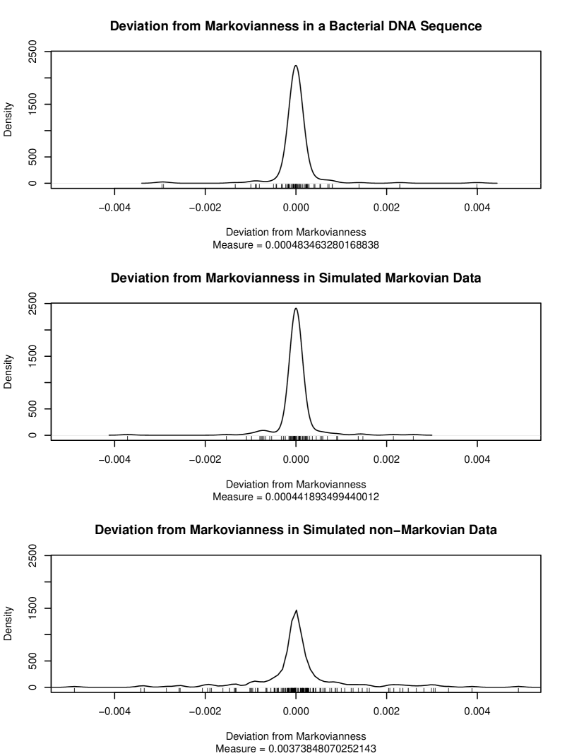
Figure 1: Empirical evidence of the efficacy of using the standard deviation as a measure of the degree by which a sequence deviates from the Markov property. The top figure pertains to the START/STOP codons annotated on the primary strand of escherichia coli K-12. The deviations are marked on the x-axis while the curve represents a kernel density estimate of the deviations. The middle plot illustrates the same thing using a simulated Markov chain. The bottom plot was produced using non-Markovian simulations of latent AR$(2)$ processes.

Figure 1 displays a kernel density estimate for $\widehat{M}_{3}$ in three cases. The first case shows the density of $\widehat{M}_{3}$ for the sequence of START/STOP codons annotated on the primary strand of the escherichia coli K-12 genome. Let us denote this sequence by $X^{1}$. The second case shows the density estimated for a sequence $X^{2}$ of START/STOP codons simulated from a Markov chain using a transition matrix estimated from $X^{1}$. The idea is that $X^{1}$ and $X^{2}$ be statistically the same for single codons and pairs of consecutive codons so that $\widehat{M}_{3}$ only highlights the kind of mechanism, Markovian or non-Markovian, driving the process. In the third case, a latent AR$(2)$ process was simulated using the following scheme.

Let $(Z_{k}:k=0,1,\ldots,n)$ be an AR$(2)$ process with autoregressive coefficients $\lambda_{1}$ and $\lambda_{2}$, that is:

$$Z_{t}=\lambda_{1}Z_{t-1}+\lambda_{2}Z_{t-2}+\epsilon_{t},$$

where the innovations $\epsilon_{t}$ are independently and identically distributed normal random variables with mean $0$ and variance $\sigma^{2}$. The process $Z$ is stationary if and only if the parameters satisfy the conditions

$$\lambda_{2}>-1,\qquad\lambda_{2}+\lambda_{1}<1\mbox{ and }\lambda_{2}-\lambda_{1}<1.$$ (3)

Note that $Z$ is a Markov chain if and only if $\lambda_{2}=0$ and an i.i.d. process if and only if $\lambda_{2}=\lambda_{1}=0$.

Next, let $q_{Z}(p)$ denote the quantile function of $Z$ , that is,

$$q_{Z}(p)=\max\left\{z\in{\mathbb{R}}\;:\;\biggl{(}\frac{1}{n}\sum_{t=0}^{n}{\bf 1}_{Z_{t}\leq z}\biggr{)}\leq p\right\}.$$

Finally, we define the stochastic process $(Y_{t}:t=0,1,\ldots,n)$. To do this, we require that the symbols in $I$ are ordered in some way. The order does not matter, we merely need to be able to say for $i,j\in I$ that either $i$ comes before $j$ or $j$ comes before $i$. Let $\underline{i}$ denote the symbol in $I$ that comes before all others in $I$. Then, the latent AR$(2)$ process is then defined as

$$Y_{t}=\left\{\begin{array}[]{ll}\underline{i}&\mbox{if }Y_{t}\leq q_{Z}(\pi_{\underline{i}}),\\ i,&\mbox{if }q_{Z}\left(\sum_{j<i}(\pi_{j})\right)<Z_{t}\leq q_{Z}\left(\sum_{j\leq i}\pi_{j})\right).\end{array}\right.$$

Due to how $Y$ has been constructed, $\pi$ is its invariant state distribution. Also, $Y$ will be Markovian if and only if $Z$ is Markovian (equivalently, $\lambda_{2}=0$).

In the third case, we simulated a sequence $X^{3}$ of START and STOP codons from the latent AR$(2)$ process described above. In order to obtain a non-Markovian sequence with the same distribution of symbols as $X^{1}$, we set $\lambda_{1}=-0.2$ and $\lambda_{2}=0.4$, and estimated $\pi$ from $X^{1}$ .

In Figure 1, the densities of the deviations $\widehat{M}_{3}$ for the sequences derived from escherichia coli and the Markov chain simulation are fairly similar. Their statistics $S_{3}$ are also comparable. In contrast, the density of $\widehat{M}_{3}$ for the non-Markovian simulation has much longer tails and exhibits much greater dispersion. The x-axis of the third plot in the figure has been truncated to the interval $[0.005,0.005]$ to maintain clarity and allow for easy comparison with the other two densities. All three graphs have been plotted on the same scale also for this reason. Prior to truncation, the density of $\widehat{M}_{3}$ for the non-Markovian sample spanned the interval $[-0.0195,0.0327]$ and 14 data points are omitted by the truncation. The measure $S_{3}$ for the simulated latent AR$(2)$ process is almost an order of magnitude larger than it is for the other two cases.

Table 3: A measure of Markovianness based on a trinucleotide analysis applied to the annotated START and STOP codons on the primary strand sequences of bacterial genomes, together with Markovian and non-Markovian simulations. The Markovian simulations have statistically equivalent dinucleotide distributions to the annotated STARTs/STOPs while the non-Markovian simulations have the same mononucleotide distributions as their bacterial counterparts.

Chromosome	Measure from			Number of
	Genome	Markovian	Non-Markovian	STARTs
		Simulations	Simulations	and STOPs
Escherichia coli str. K-12 substr. MG1655	0.000483	0.000379	0.003977	4058
Helicobacter pylori 26695 chromosome	0.000617	0.000798	0.003590	1528
Staphylococcus aureus subsp. aureus MRSA252 chromosome	0.000654	0.000487	0.003731	2560
Leptospira interrogans serovar Lai str. 56601 chromosome I	0.000695	0.000527	0.003230	3626
Leptospira interrogans serovar Lai str. 56601 chromosome II	0.002731	0.001805	0.004268	320
Streptococcus pneumoniae ATCC 700669	0.000801	0.000579	0.003776	1910
Bacillus subtilis subsp. spizizenii str. W23 chromosome, complete	0.000373	0.000495	0.003509	3844
Vibrio cholerae O1 str. 2010EL-1786 chromosome 1	0.000715	0.000543	0.003598	2750
Vibrio cholerae O1 str. 2010EL-1786 chromosome 2	0.000560	0.000836	0.003738	1162
Propionibacterium acnes TypeIA2 P.acn33 chromosome	0.000882	0.000513	0.003983	2234
Salmonella enterica subsp. enterica serovar Typhi str. P-stx-12	0.001453	0.000419	0.003632	4806
Yersinia pestis D182038 chromosome	0.000592	0.000511	0.003502	3430
Mycobacterium tuberculosis 7199-99	0.000483	0.000460	0.002453	4006

Table 4: A measure of Markovianness based on a trinucleotide analysis applied to the annotated START and STOP codons on the complementary strand sequences of bacterial genomes, together with Markovian and non-Markovian simulations. The Markovian simulations have statistically equivalent dinucleotide distributions to the annotated STARTs/STOPs while the non-Markovian simulations have the same mononucleotide distributions as their bacterial counterparts.

Chromosome	Measure from			Number of
	Genome	Markovian	Non-Markovian	STARTs
		Simulations	Simulations	and STOPs
Escherichia coli str. K-12 substr. MG1655	0.000786	0.000353	0.004120	4284
Helicobacter pylori 26695 chromosome	0.001364	0.000766	0.003741	1606
Staphylococcus aureus subsp. aureus MRSA252 chromosome	0.000748	0.000455	0.003839	2730
Leptospira interrogans serovar Lai str. 56601 chromosome I	0.000736	0.000571	0.003334	3192
Leptospira interrogans serovar Lai str. 56601 chromosome II	0.001676	0.001921	0.004303	266
Streptococcus pneumoniae ATCC 700669	0.000587	0.000588	0.003635	2070
Bacillus subtilis subsp. spizizenii str. W23 chromosome	0.000521	0.000468	0.003460	4276
Vibrio cholerae O1 str. 2010EL-1786 chromosome 1	0.001121	0.000526	0.003552	2860
Vibrio cholerae O1 str. 2010EL-1786 chromosome 2	0.000750	0.000976	0.003687	918
Propionibacterium acnes TypeIA2 P.acn33 chromosome, complete	0.000949	0.000528	0.003908	2232
Salmonella enterica subsp. enterica serovar Typhi str. P-stx-12	0.000705	0.000417	0.003508	4574
Yersinia pestis D182038 chromosome	0.000644	0.000497	0.003606	3810
Mycobacterium tuberculosis 7199-99	0.000509	0.000461	0.002546	3962

Table 3 displays the value of $S_{3}$ computed on the primary strand of 13 bacterial DNA sequences. The second column shows $S_{3}$ derived from genome annotation data. The third and fourth columns show the measure of deviation from Markovianness as applied to Markovian and non-Markovian sequences respectively simulated as described above. For each of these columns, a sequence of the same length as the annotated START/STOP codons was simulated $1000$ times and the mean value of $S_{3}$ over the $1000$ replications is shown in the table. For the non-Markovian case, the autoregressive parameters $\lambda_{1}$ and $\lambda_{2}$ were selected uniformly at random from the set of values that give rise to a stationary AR$(2)$ process for each simulation. It is quite evident that the values of $S_{3}$ for the annotation data and the Markovian simulations are of the same order of magnitude while the non-Markovian simulations result in values of $S_{3}$ that are from two times to an order of magnitude greater. The final column in the table shows the length of the sequence of START and STOP codons annotated for each of the DNA sequences. There appears to be no relationship between the sequence length and any of the measures of deviation from Markovianness calculated. Performing the same analysis on the complementary strands yields similar results which are shown in Table 4.

Table 5: A measure of Markovianness based on a quadranucleotide analysis applied to the annotated START and STOP codons on the primary strand sequences of bacterial genomes, together with Markovian and non-Markovian simulations. The Markovian simulations have statistically equivalent dinucleotide distributions to the annotated STARTs/STOPs while the non-Markovian simulations have the same mononucleotide distributions as their bacterial counterparts.

\̧centering Chromosome Measure from Number of Genome Markovian Non-Markovian STARTs Simulations Simulations and STOPs Escherichia coli str. K-12 substr. MG1655 0.000199 0.000188 0.001399 4058 Helicobacter pylori 26695 chromosome 0.000408 0.000404 0.001213 1528 Staphylococcus aureus subsp. aureus
MRSA252 chromosome 0.000339 0.000253 0.001236 2560 Leptospira interrogans serovar Lai str. 56601 chromosome I 0.000338 0.000266 0.001084 3626 Leptospira interrogans serovar Lai str. 56601 chromosome II 0.001170 0.000904 0.001566 320 Streptococcus pneumoniae
ATCC 700669 0.000380 0.000280 0.001268 1910 Bacillus subtilis subsp. spizizenii str. W23 chromosome 0.000249 0.000251 0.001054 3844 Vibrio cholerae O1 str. 2010EL-1786 chromosome 1 0.000322 0.000270 0.001208 2750 Vibrio cholerae O1 str. 2010EL-1786 chromosome 2 0.000397 0.000425 0.001228 1162 Propionibacterium acnes TypeIA2 P
.acn33 chromosome 0.000325 0.000271 0.001427 2234 Salmonella enterica subsp. enterica serovar Typhi str. P-stx-12 0.000513 0.000206 0.001218 4806 Yersinia pestis D182038 chromosome 0.000297 0.000257 0.001101 3430 Mycobacterium tuberculosis 7199-99 0.000240 0.000212 0.000706 4006

Table 6: A measure of Markovianness based on a quadranucleotide analysis applied to the annotated START and STOP codons on the complementary strand sequences of bacterial genomes, together with Markovian and non-Markovian simulations. The Markovian simulations have statistically equivalent dinucleotide distributions to the annotated STARTs/STOPs while the non-Markovian simulations have the same mononucleotide distributions as their bacterial counterparts.

Chromosome	Measure from			Number of
	Genome	Markovian	Non-Markovian	STARTs
		Simulations	Simulations	and STOPs
Escherichia coli str. K-12 substr. MG1655	0.000307	0.000179	0.001372	4284
Helicobacter pylori 26695 chromosome	0.000500	0.000378	0.001157	1606
Staphylococcus aureus subsp. aureus MRSA252 chromosome	0.000259	0.000243	0.001195	2730
Leptospira interrogans serovar Lai str. 56601 chromosome I	0.000369	0.000287	0.001067	3192
Leptospira interrogans serovar Lai str. 56601 chromosome II	0.000857	0.000973	0.001650	266
Streptococcus pneumoniae ATCC 700669	0.000302	0.000282	0.001251	2070
Bacillus subtilis subsp. spizizenii str. W23 chromosome	0.000244	0.000234	0.001092	4276
Vibrio cholerae O1 str. 2010EL-1786 chromosome 1	0.000478	0.000266	0.001160	2860
Vibrio cholerae O1 str. 2010EL-1786 chromosome 2	0.000443	0.000485	0.001274	918
Propionibacterium acnes TypeIA2 P.acn33 chromosome	0.000398	0.000274	0.001367	2232
Salmonella enterica subsp. enterica serovar Typhi str. P-stx-12	0.000395	0.000216	0.001165	4574
Yersinia pestis D182038 chromosome	0.000274	0.000244	0.001182	3810
Mycobacterium tuberculosis 7199-99	0.000220	0.000213	0.000731	3962

We can also consider Markovianness in terms of quadranucleotides. In this case, $[ijkl]$ is the cylinder set for quadranucleotide $ijkl$. We define

$$M_{4}(i,j,k,l)={\mathbb{P}}([ijkl])-\frac{{\mathbb{P}}([ijk]){\mathbb{P}}([kl])}{{\mathbb{P}}([k])},\qquad i,j,k,l\in I.$$

Now, if $X_{t}$ is be Markovian then $M_{4}(i,j,k,l)=0$ for all $i,j,k,l\in I$. Once again, we note that for most of the bacteria we examined, the alternating nature of their sequences of START and STOP codons means that a minimum of 1134 elements of $M_{4}=(M_{4}(i,j,k):i,j,k,l\in I)$ will be zero, regardless of whether or not the sequence of STARTs and STOPs is Markovian. In a manner similar to the case for $M_{3}$, we can estimate $M_{4}(i,j,k,l)$ by

$$\widehat{M}_{4}(i,j,k,l)=\frac{N_{ijkl}}{n}-\frac{N_{ijk}N_{kl}}{nN_{k}}.$$

Furthermore, the mean $\bar{\widehat{M}}_{4}=0$ and

$$S_{4}=\sigma(\widehat{M}_{4})=\sum_{i,j,k,l\in I}\widehat{M}_{4}(i,j,k,l)^{2}$$

constitutes a measure of deviation from Markovianness in terms of quadranucleotides analogously to $S_{3}$ for trinucleotides.

We repeated the experiments for trinucleotides shown in Tables 3 and 4, but using $S_{4}$ instead of $S_{3}$ as the measure of deviation from Markovianness. The results on the primary strand are displayed in Table 5 while those on the complementary strand appear in Table 6.

3 Further structure of the Markov chain

3.1 Markov chain with partitioned transition matrices

Let $I$ be the set of START and STOP codon symbols and $Q=(Q_{ij}:i,j\in I)$ be the stochastic matrix of the Markov chain generating the sequence of annotated START and STOP codons. Its stationary vector will be denoted by $\pi=(\pi_{i}:i\in I)$. The entropy $h(Q,\pi)$ of this stationary Markov chain is

$$h(Q,\pi)=-\sum_{(i,j)\in I\times I}\pi_{i}q_{ij}\log q_{ij}.$$ (4)

The set $I$ is partitioned into two disjoint sets: the set of START codons $I_{0}$ and the set of STOP codons $I_{1}$. Then, $Q$ has the form

$$Q=\left(\begin{array}[]{cc}0&Q^{0}\\ Q^{1}&0\end{array}\right)$$ (5)

That is $q_{ij}=0$ if $\{i,j\}\subseteq I_{0}$ or if $\{i,j\}\subseteq I_{1}$. the matrix $Q^{0}$ is of dimension $|I_{0}|\times|I_{1}|$ while $Q^{1}$ is a $|I_{1}|\times|I_{0}|$ matrix. It is convenient to set

$$\Delta=I_{0}\times I_{1}\cup I_{1}\times I_{0}.$$

The Markov measure ${\mathbb{P}}(X_{k}=i_{k},k=0,..,m)=\pi_{i_{k}}\prod_{k=0}^{m-1}q_{i_{k}i_{k+1}}$ can give positive weight only to those trajectories with $(i_{k},i_{k+1})\in\Delta$ for all $k=0,..,m-1$. In this case the entropy formula satisfies

$$h(Q,\pi)=-\sum_{(i,j)\in\Delta}\pi_{i}q_{ij}\log q_{ij}.$$

Since $Q$ is stochastic, the row sums of the matrices $Q^{0}$ and $Q^{1}$ are equal to $1$. Let ${\bf 1}_{I_{l}}$ be a unitary vector of dimension $|I_{l}|$ for $l=0,1$. Then, $Q^{0}{\bf 1}_{I_{1}}={\bf 1}_{I_{0}}$ and $Q^{1}{\bf 1}_{I_{0}}={\bf 1}_{I_{1}}$. We can assume that the matrices $Q^{1}Q^{0}$ and $Q^{0}Q^{1}$ are strictly positive, which ensures that $Q$ is irreducible. Let $\pi$ be the unique stationary vector, we denote $\pi_{I_{l}}=(\pi_{i}:i\in I_{l})$ for $l=0,1$. The stationary condition is $\pi^{t}Q=\pi^{t}$, which is equivalent to $\pi_{I_{0}}^{t}=\pi_{I_{1}}^{t}Q^{1}$ and $\pi_{I_{1}}^{t}=\pi_{I_{0}}^{t}Q^{0}$. Hence,

$$\pi_{I_{0}}^{t}=\pi_{I_{0}}^{t}Q^{0}Q^{1}\hbox{ and }\pi_{I_{1}}^{t}=\pi_{I_{1}}^{t}Q^{1}Q^{0}.$$ (6)

The strictly positive matrices $Q^{1}Q^{0}$ and $Q^{0}Q^{1}$ are stochastic, so there exist positive solutions $\pi_{I_{0}}$ and $\pi_{I_{1}}$ to (6) and we require two normalization conditions. The first one is $\pi_{I_{0}}^{t}{\bf 1}_{I_{0}}+\pi_{I_{1}}^{t}{\bf 1}_{I_{1}}=1$, that is $\sum_{i\in I_{0}}\pi_{i}+\sum_{i\in I_{1}}\pi_{i}=1$. The second condition is

$$\pi_{I_{0}}^{t}{\bf 1}_{I_{0}}=\pi_{I_{1}}^{t}Q^{1}{\bf 1}_{I_{0}}=\pi_{I_{1}}^{t}{\bf 1}_{I_{1}}.$$

That is $\sum_{i\in I_{0}}\pi_{i}=\sum_{i\in I_{1}}\pi_{i}$, and so it is equal to $1/2$. Hence the probability vector $\pi$ is uniquely determined.

3.2 Conditional Independence

It will be useful to set $I_{l}=I_{0}$ when $l$ is even and $I_{l}=I_{1}$ when $l$ is odd. In the sequel let $l$ be $0$ or $1$. The sequence $(X_{n}:n\geq 0)$ is conditionally independent given $X_{0}\in I_{l}$ if and only if for all $m\geq 0$ and all $i_{k}\in I_{l+k}$, $k=0,..,m$, we have

$${\mathbb{P}}(X_{k}=i_{k},k=0,..,m|X_{0}\in I_{l})=\prod_{k=0}^{m}{\mathbb{P}}(X_{k}=i_{k}|X_{0}\in I_{l}).$$ (7)

This equality is easily seen to be equivalent to

$$2\pi_{i_{l}}\prod_{k=0}^{m-1}q_{i_{k+l}i_{k+1+l}}=2^{m+1}\prod_{k=0}^{m}\pi_{i_{k}}.$$

From this relation it can be concluded that a necessary and sufficient condition for conditional independence is

$$\forall\,i,j\in I:\quad q_{ij}=2\pi_{j}{\bf 1}_{(i,j)\in\Delta}.$$

When there is conditional independence, and to avoid any confusion, the transition matrix will be denoted $Q^{\dagger}=(q^{\dagger}_{ij}:i,j\in I)$, so $q^{\dagger}_{ij}=2\pi_{j}{\bf 1}_{(i,j)\in\Delta}$. In this case the invariant distribution is also $\pi$. We have

$$h(Q^{\dagger},\pi)=-\sum_{(i,j)\in\Delta}2\pi_{i}\pi_{j}\log 2\pi_{j}=-\log 2+h_{\pi},$$ (8)

where we noted $h_{\pi}=-\sum_{i\in I}\pi_{i}\log\pi_{i}$ and we used $\sum_{i\in I_{l}}\pi_{i}=1/2$ and $\sum_{(i,j)\in\Delta}\pi_{i}\pi_{j}=1/2$.

Remark. In a similar way, we could also define conditional independence given the event $X_{k}\in I_{l+k}$, $k=0,..,s$, but the equality

$${\mathbb{P}}(X_{k}=i_{k},k=0,..,m|X_{k}\in I_{l+k},k=0,..,s)={\mathbb{P}}(X_{k}=i_{k},k=0,..,m|X_{0}\in I_{l})$$

for $m\geq s$ means that this definition is equivalent to conditional independence given $X_{0}\in I_{l}$.

3.3 Kullback-Leibler divergence and mutual information in the conditional case

Let ${\bf P}$ be the joint distribution of $(X_{k},X_{k+1})$ on $I\times I$ for some $k\geq 0$. By stationarity it does not depend on $k$. We write ${\bf P}(i,j)={\mathbb{P}}((X_{k},X_{k+1}=(i,j))$ for $(i,j)\in I\times I$. Note that

$${\bf P}(i,j)=\pi_{i}q_{ij}{\bf 1}_{(i,j)\in\Delta}.$$

So, ${\bf P}$ is supported by $\Delta$. The entropy of the measure ${\bf P}$ on $I\times I$ is:

$$h({\bf P})=-\sum_{(i,j)\in I\times I}\pi_{i}q_{ij}\log(\pi_{i}q_{ij})=h(Q,\pi)+h_{\pi}.$$ (9)

Let us consider ${\bf P}^{\dagger}$ as the bivariate distribution under conditional independence. Then,

$${\bf P}^{\dagger}(i,j)=\pi_{i}q^{\dagger}_{ij}{\bf 1}_{(i,j)\in\Delta}=2\pi_{i}\pi_{j}{\bf 1}_{(i,j)\in\Delta}.$$

The entropy of the joint distribution ${\bf P}^{\dagger}$ is

$$h({\bf P}^{\dagger})=-\sum_{(i,j)\in\Delta}2\pi_{i}\pi_{j}\log(2\pi_{i}\pi_{j})=-\log 2-2\sum_{i\in I}\pi_{i}\log\pi_{i}=-\log 2+2h_{\pi}.$$

Let us consider the Kullback-Leibler divergence of ${\bf P}^{\dagger}$ from ${\bf P}$. By definition, the divergence is

$$D_{\mathrm{KL}}\left({{\bf P}}\|{{\bf P}^{\dagger}}\right)=\sum_{i\in I,j\in I}{\bf P}(i,j)\log({\bf P}(i,j)/{\bf P}^{\dagger}(i,j)).$$

In our case an easy computation shows that

$$D_{\mathrm{KL}}\left({{\bf P}}\|{{\bf P}^{\dagger}}\right)=-\log 2+2h_{\pi}-h({\bf P}).$$

These equalities, together with formulae (4), (8) and (9) give

$$D_{\mathrm{KL}}\left({{\bf P}}\|{{\bf P}^{\dagger}}\right)=h(Q^{\dagger},\pi)-h(Q,\pi).$$

As ${\bf P}$ and ${\bf P}^{\dagger}$ are proper probability distributions, Gibbs’ inequality yields $D_{\mathrm{KL}}\left({{\bf P}}\|{{\bf P}^{\dagger}}\right)\geq 0$. Since we assume $Q^{0}$ and $Q^{1}$ are strictly positive matrices, the distributions ${\bf P}$ and ${\bf P}^{\dagger}$ have the same support $\Delta$. Then, we have that the inequality $D_{\mathrm{KL}}\left({{\bf P}}\|{{\bf P}^{\dagger}}\right)\geq 0$ becomes a strict equality $D_{\mathrm{KL}}\left({{\bf P}}\|{{\bf P}^{\dagger}}\right)=0$ if and only if ${\bf P}={\bf P}^{\dagger}$. Consequently, $D_{\mathrm{KL}}\left({{\bf P}}\|{{\bf P}^{\dagger}}\right)=h(Q^{\dagger},\pi)-h(Q,\pi)$ provides us a way to measure how closely ${\mathbb{P}}$ complies with the notion of conditional independence described above.

We can interpret the above result in terms of mutual information. Let $\pi\otimes\pi$ be the product probability measure on $I\times I$. The mutual information of the distribution  ${\bf P}$ of $(X_{k},X_{k+1})$ on $I\times I$ satisfies:

$$I({\bf P})=\sum_{(i,j)\in I\times I}{\bf P}(i,j)\log\frac{{\bf P}(i,j)}{\pi\otimes\pi(i,j)}=\sum_{(i,j)\in\Delta}\pi_{i}q_{ij}\log\frac{\pi_{i}q_{ij}}{\pi_{i}\pi_{j}}=h_{\pi}-h(Q,\pi).$$

It follows that

$$D_{\mathrm{KL}}\left({{\bf P}}\|{{\bf P}^{\dagger}}\right)=I({\bf P})-\log 2.$$

Therefore, the mutual information is bounded below by $\log 2$. Further, attainment of this lower bound by $I({\bf P})$ is equivalent to $D_{\mathrm{KL}}\left({{\bf P}}\|{{\bf P}^{\dagger}}\right)=0$, that is, conditional independence of the sequence $(X_{n}:n\in{\mathbb{N}})$ given $X_{0}\in I_{l}$ for some $l\in\{0,1\}$. Indeed, $\log 2$ is the mutual information of conditionally independent random variables:

$$I({\bf P}^{\dagger})=\sum_{(i,j)\in\Delta}2\pi_{i}\pi_{j}\log\frac{2\pi_{i}\pi_{j}}{\pi_{i}\pi_{j}}=\sum_{(i,j)\in\Delta}2\pi_{i}\pi_{j}\log 2=\log 2.$$

Thus, $D_{\mathrm{KL}}\left({{\bf P}}\|{{\bf P}^{\dagger}}\right)=I({\bf P})-I({\bf P}^{\dagger})$. The divergence of ${\bf P}^{\dagger}$ from ${\bf P}$ may thus be viewed as the difference in mutual information of ${\bf P}$ and ${\bf P}^{\dagger}$.

Remark.

To consider the case in which there are more than two classes of codons, let $I=I_{0}\cup I_{1}\cup\cdots\cup I_{d-1}$ where $d>1$. Suppose that $Q_{k}$, $k=0,1,\ldots,d-1$ is a collection of stochastic matrices and that $Q$ has the form

$$Q=\begin{pmatrix}0&Q^{0}&0&\cdots&0\\ 0&0&Q^{1}&\cdots&0\\ \vdots&\vdots&\vdots&&\vdots\\ 0&0&0&\cdots&Q^{d-2}\\ Q^{d-1}&0&0&\cdots&0\end{pmatrix}.$$

then the above discussion remains valid for $Q$ by replacing $\log 2$ by $\log d$ and $\Delta$ by

$$\Delta=\bigcup_{l=0}^{d-1}I_{l}\times I_{l+1}\times\cdots\times I_{l+d-1}$$

where we set $I_{s+rd}=I_{s}$ for $s=0,\ldots,d-1$, $r\geq 0$. $\Box$

Table 7: Entropies, Kullback-Leibler divergences and relative difference in entropies for the Markov chain producing the sequence of START and STOP codons on the primary strand of 13 bacterial chromosomes.

Chromosome	Entropy	Entropy	K-L Div	Rel. Diff.
	$h(Q,\pi)$	$h(Q^{\dagger},\pi)$		(%)
Escherichia coli str. K-12 substr. MG1655	0.5987	0.5991	0.0004	0.04
Helicobacter pylori 26695 chromosome	0.7986	0.7994	0.0008	0.05
Staphylococcus aureus subsp. aureus MRSA252 chromosome	0.6738	0.6751	0.0013	0.10
Leptospira interrogans serovar Lai str. 56601 chromosome I	0.8084	0.8104	0.0020	0.13
Leptospira interrogans serovar Lai str. 56601 chromosome II	0.8107	0.8224	0.0116	0.71
Streptococcus pneumoniae ATCC 700669,	0.6317	0.6323	0.0006	0.05
Bacillus subtilis subsp. spizizenii str. W23 chromosome	0.7957	0.7968	0.0011	0.07
Vibrio cholerae O1 str. 2010EL-1786 chromosome 1	0.7323	0.7350	0.0027	0.19
Vibrio cholerae O1 str. 2010EL-1786 chromosome 2	0.7473	0.7554	0.0081	0.54
Propionibacterium acnes TypeIA2 P.acn33 chromosome	0.6375	0.6424	0.0049	0.38
Salmonella enterica subsp. enterica serovar Typhi str. P-stx-12	0.7226	0.7237	0.0012	0.08
Yersinia pestis D182038 chromosome	0.7679	0.7695	0.0016	0.10
Mycobacterium tuberculosis 7199-99	0.9113	0.9130	0.0017	0.09

Table 8: Entropies, Kullback-Leibler divergences and relative difference in entropies for the Markov chain producing the sequence of START and STOP codons on the complementary strand of 13 bacterial chromosomes.

Chromosome	Entropy	Entropy	K-L Div	Rel. Diff.
	$h(Q,\pi)$	$h(Q^{\dagger},\pi)$		(%)
Escherichia coli str. K-12 substr. MG1655	0.5801	0.5816	0.0015	0.13
Helicobacter pylori 26695 chromosome.	0.7734	0.7771	0.0037	0.24
Staphylococcus aureus subsp. aureus MRSA252 chromosome	0.6597	0.6611	0.0014	0.11
Leptospira interrogans serovar Lai str. 56601 chromosome I	0.8187	0.8200	0.0013	0.08
Leptospira interrogans serovar Lai str. 56601 chromosome II	0.8078	0.8350	0.0272	1.66
Streptococcus pneumoniae ATCC 700669	0.6462	0.6491	0.0029	0.22
Bacillus subtilis subsp. spizizenii str. W23 chromosome	0.7878	0.7885	0.0007	0.04
Vibrio cholerae O1 str. 2010EL-1786 chromosome 1	0.7320	0.7343	0.0023	0.16
Vibrio cholerae O1 str. 2010EL-1786 chromosome 2	0.7491	0.7634	0.0143	0.95
Propionibacterium acnes TypeIA2 P.acn33 chromosome	0.6474	0.6493	0.0019	0.15
Salmonella enterica subsp. enterica serovar Typhi str. P-stx-12	0.7272	0.7276	0.0004	0.03
Yersinia pestis D182038 chromosome	0.7607	0.7641	0.0034	0.22
Mycobacterium tuberculosis 7199-99	0.9052	0.9071	0.0019	0.10

For both strands, we calculated the entropies $h(Q,\pi)$ and $h(Q^{\dagger},\pi)$, as l as the Kullback-Leibler divergence and the relative difference between the entropies expressed as a percentage. All of these values a summarized in Tables 7 and 8. The Kullback-Lebler divergences and the relative differences between the entropies are all very close to zero, which is precisely what one expects to see if $(X_{n}:n\in{\mathbb{N}})$ is conditionally independent given $X_{0}\in I_{l}$ for some $l\in\{0,1\}$.

We need to mention that the transition matrices for escherichia coli K-12 violate the exact form of $Q$ (see the comments in the first section of the appendix). They possess some non-zero elements in the top-left quadrant of the matrix. In order to calculate the quantities shown in Tables 7 and 8, it was necessary to set the offending elements to zero and rescale the affected rows to sum to unity.

Table 9: Maximum absolute difference between START/STOP frequencies on the two strands in the DNA duplexes of 13 bacterial chromosomes. the last column displays the number of annotated START/STOP codons present in the duplex.

Chromosome	Maximum Absolute	Corr.	Number of
	Difference in Frequency	Coef.	Codons
Escherichia coli str. K-12 substr. MG1655	0.0095	0.9995	8342
Helicobacter pylori 26695 chromosome	0.0104	0.9994	3134
Staphylococcus aureus subsp. aureus MRSA252 chromosome	0.0123	0.9988	5290
Leptospira interrogans serovar Lai str. 56601 chromosome I	0.0093	0.9993	6818
Leptospira interrogans serovar Lai str. 56601 chromosome II	0.0240	0.9932	586
Streptococcus pneumoniae ATCC 700669	0.0189	0.9983	3980
Bacillus subtilis subsp. spizizenii str. W23 chromosome	0.0083	0.9991	8120
Vibrio cholerae O1 str. 2010EL-1786 chromosome 1	0.0122	0.9985	5610
Vibrio cholerae O1 str. 2010EL-1786 chromosome 2	0.0420	0.9825	2080
Propionibacterium acnes TypeIA2 P.acn33 chromosome	0.0046	0.9999	4466
Salmonella enterica subsp. enterica serovar Typhi str. P-stx-12	0.0219	0.9961	9380
Yersinia pestis D182038 chromosome	0.0044	0.9998	7240
Mycobacterium tuberculosis 7199-99	0.0069	0.9993	7968

3.4 Chargaff’s second parity rule

Finally, we have observed that the annotated START and STOP codons taken together from both the primary and complementary strands essentially comply with Chargaff’s second parity rule. Chargaff’s first parity rule [3] says that, within a DNA duplex, the numbers of $A$ and $T$ mononucleotides are the same while the numbers of $C$ and $G$ nucleotides also agree. Chargaff’s second parity rule not only says this continues to hold within a DNA simplex, but rather that short oligonucleotides and their reverse complements appear with the same frequency within a simplex [10]. Firstly, note that within a DNA duplex, the START and STOP codons on one strand correspond to their reverse complements on the other strand. Consequently, we can perform basic checks for compliance with Chargaff’s second parity rule by considering both the difference and correlation between the frequencies of every START and STOP codon in each strand. If we let $\pi^{(1)}=(\pi_{i}^{(1)}:i\in I)$ and $\pi^{(2)}=(\pi_{i}^{(2)}:i\in I)$ be the frequencies of the symbols in $I$ on the primary and complementary strands respectively. Of course, $\pi^{(1)}$ and $\pi^{(2)}$ constitute the stationary distributions of the chains of START and STOP codons on their corresponding strands. The $\ell_{\infty}$ distance between these two probability vectors, given by

$$\left\|{\pi^{(1)}-\pi^{(2)}}\right\|_{\infty}=\max_{i\in I}\left|{\pi_{i}^{(1)}-\pi_{i}^{(2)}}\right|,$$

together with their sample correlation coefficient $\mathop{\rm corr}\left(\pi^{(1)},\pi^{(2)}\right)$, will indicate how closely the trinucleotide frequencies conform to Chargaff’s second parity rule.

Table 9 shows $\left\|{\pi^{(1)}-\pi^{(2)}}\right\|_{\infty}$ and $\mathop{\rm corr}\left(\pi^{(1)},\pi^{(2)}\right)$ for each of the 13 DNA sequences we have examined. the values shown in the table indicate a high degree of compliance by the START/STOP sequences with Chargaff’s second parity rule. The last column of the table shows the number of codons in the DNA duplex of each chromosome. The annotated START and STOP codons in the bacterial duplexes examined constitute between 1578 and 28140 nucleotides with a mean average of 16848. Generally speaking, this is equivalent to discovering Chargaff’s second parity rule in short sequences, but the level of compliance based on the correlation (0.9825–0.9999)we have observed for START/STOP codon sequences appears high for the quantity of nucleotides. It is instructive to compare this to that reported in Figure 4a of [1] for nucleotide sequence segments of comparable size taken from human chromosome 1, but with two caveats. Firstly, note that the correlations reported in Table 9 are based on the vectors $\pi^{(1)}$ and $\pi^{(2)}$, which are of length 6 or 7 for the bacteria studied here, whereas Albrecht-Buehler’s correlations are based on vectors containing the counts for 64 trinucleotides. This may partly account for the high levels of compliance and small variance seen here, even for very short codon sequences. Secondly, we are comparing intrastrand codon correlations or prokaryotes against those for a eukaryote chromosome, which strictly speaking should not be comparable since they may respond in different ways to varying quantities of nucleotides.

Appendix: Estimated transition matrices for 13 bacterial genomes

1. Escherichia coli str. K-12 substr. MG1655, complete genome.

   In the estimated START/STOP transition matrices for the primary and complementary strands of Escherichia Coli K-12, there appear two anomalous entries in the top-left corner of each matrix. Inspection of the annotation (NC_000913.2) available from GenBank reveals that the 603rd gene on the primary strand spans loci 1204594–1205365 relative to the $5^{\prime}$ end it starts with GTG and finishes with an ATG codon.

   Similarly, the two non-zero elements in the top-left corner of the transition matrix estimated for the complementary strand are explained by the 473rd gene on the complementary strand. This gene spans loci 1077648–1077866 relative to the $5^{\prime}$ end of the complementary strand. It starts with an ATG codon and finishes with a GTG codon.

   Primary Strand

   	ATG	GTG	TTG	TAA	TAG	TGA
   ATG	0.0005	0.0000	0.0000	0.6481	0.0784	0.2729
   GTG	0.0063	0.0000	0.0000	0.6266	0.0823	0.2848
   TTG	0.0000	0.0000	0.0000	0.6389	0.0833	0.2778
   TAA	0.8994	0.0831	0.0175	0.0000	0.0000	0.0000
   TAG	0.8875	0.0938	0.0187	0.0000	0.0000	0.0000
   TGA	0.9209	0.0612	0.0180	0.0000	0.0000	0.0000

   Complementary Strand

   	ATG	GTG	TTG	TAA	TAG	TGA
   ATG	0.0000	0.0005	0.0000	0.6572	0.0556	0.2867
   GTG	0.0061	0.0000	0.0000	0.5521	0.0982	0.3436
   TTG	0.0000	0.0000	0.0000	0.5405	0.1081	0.3514
   TAA	0.9135	0.0707	0.0159	0.0000	0.0000	0.0000
   TAG	0.8984	0.0781	0.0234	0.0000	0.0000	0.0000
   TGA	0.8946	0.0863	0.0192	0.0000	0.0000	0.0000

2. Helicobacter pylori 26695 chromosome, complete genome.

   Primary Strand

   	ATG	GTG	TTG	TAA	TAG	TGA
   ATG	0.0000	0.0000	0.0000	0.5563	0.1688	0.2749
   GTG	0.0000	0.0000	0.0000	0.4750	0.2000	0.3250
   TTG	0.0000	0.0000	0.0000	0.5323	0.1935	0.2742
   TAA	0.8106	0.1103	0.0791	0.0000	0.0000	0.0000
   TAG	0.8120	0.0977	0.0902	0.0000	0.0000	0.0000
   TGA	0.8224	0.0981	0.0794	0.0000	0.0000	0.0000

   Complementary Strand

   	ATG	GTG	TTG	TAA	TAG	TGA
   ATG	0.0000	0.0000	0.0000	0.5852	0.1493	0.2655
   GTG	0.0000	0.0000	0.0000	0.4583	0.1944	0.3472
   TTG	0.0000	0.0000	0.0000	0.5000	0.2500	0.2500
   TAA	0.8374	0.0879	0.0747	0.0000	0.0000	0.0000
   TAG	0.7692	0.1077	0.1231	0.0000	0.0000	0.0000
   TGA	0.8349	0.0826	0.0826	0.0000	0.0000	0.0000

3. Staphylococcus aureus subsp. aureus MRSA252 chromosome, complete

   Primary Strand

   	ATG	GTG	TTG	TAA	TAG	TGA
   ATG	0.0000	0.0000	0.0000	0.7486	0.1434	0.1080
   GTG	0.0000	0.0000	0.0000	0.7184	0.1748	0.1068
   TTG	0.0000	0.0000	0.0000	0.7023	0.1221	0.1756
   TAA	0.8219	0.0780	0.1001	0.0000	0.0000	0.0000
   TAG	0.7880	0.0924	0.1196	0.0000	0.0000	0.0000
   TGA	0.8231	0.0816	0.0952	0.0000	0.0000	0.0000

   Complementary Strand

   	ATG	GTG	TTG	TAA	TAG	TGA
   ATG	0.0000	0.0000	0.0000	0.7276	0.1601	0.1123
   GTG	0.0000	0.0000	0.0000	0.7767	0.1262	0.0971
   TTG	0.0000	0.0000	0.0000	0.6460	0.1858	0.1681
   TAA	0.8483	0.0748	0.0768	0.0000	0.0000	0.0000
   TAG	0.8165	0.0872	0.0963	0.0000	0.0000	0.0000
   TGA	0.8354	0.0633	0.1013	0.0000	0.0000	0.0000

4. Leptospira interrogans serovar Lai str. 56601 chromosome I,

   Primary Strand

   	ATG	GTG	TTG	TAA	TAG	TGA
   ATG	0.0000	0.0000	0.0000	0.5717	0.1278	0.3004
   GTG	0.0000	0.0000	0.0000	0.6371	0.1694	0.1935
   TTG	0.0000	0.0000	0.0000	0.5338	0.1673	0.2989
   TAA	0.7892	0.0609	0.1499	0.0000	0.0000	0.0000
   TAG	0.7500	0.0968	0.1532	0.0000	0.0000	0.0000
   TGA	0.7646	0.0697	0.1657	0.0000	0.0000	0.0000

   Complementary Strand

   	ATG	GTG	TTG	TAA	TAG	TGA
   ATG	0.0000	0.0000	0.0000	0.5846	0.1230	0.2923
   GTG	0.0000	0.0000	0.0000	0.5000	0.1944	0.3056
   TTG	0.0000	0.0000	0.0000	0.5704	0.1480	0.2816
   TAA	0.7663	0.0598	0.1739	0.0000	0.0000	0.0000
   TAG	0.7299	0.0806	0.1896	0.0000	0.0000	0.0000
   TGA	0.7570	0.0774	0.1656	0.0000	0.0000	0.0000

5. Leptospira interrogans serovar Lai str. 56601 chromosome II,

   Primary Strand

   	ATG	GTG	TTG	TAA	TAG	TGA
   ATG	0.0000	0.0000	0.0000	0.5372	0.1405	0.3223
   GTG	0.0000	0.0000	0.0000	0.6000	0.0000	0.4000
   TTG	0.0000	0.0000	0.0000	0.6207	0.1034	0.2759
   TAA	0.7303	0.0562	0.2135	0.0000	0.0000	0.0000
   TAG	0.8500	0.1000	0.0500	0.0000	0.0000	0.0000
   TGA	0.7647	0.0588	0.1765	0.0000	0.0000	0.0000

   Complementary Strand

   	ATG	GTG	TTG	TAA	TAG	TGA
   ATG	0.0000	0.0000	0.0000	0.6186	0.1237	0.2577
   GTG	0.0000	0.0000	0.0000	0.1111	0.2222	0.6667
   TTG	0.0000	0.0000	0.0000	0.6667	0.1481	0.1852
   TAA	0.7089	0.0506	0.2405	0.0000	0.0000	0.0000
   TAG	0.6667	0.1111	0.2222	0.0000	0.0000	0.0000
   TGA	0.8056	0.0833	0.1111	0.0000	0.0000	0.0000

6. Streptococcus pneumoniae ATCC 700669, complete genome.

   Primary Strand

   	ATG	GTG	TTG	TAA	TAG	TGA
   ATG	0.0000	0.0000	0.0000	0.6375	0.2071	0.1554
   GTG	0.0000	0.0000	0.0000	0.6667	0.2308	0.1026
   TTG	0.0000	0.0000	0.0000	0.6383	0.2340	0.1277
   TAA	0.9049	0.0443	0.0508	0.0000	0.0000	0.0000
   TAG	0.9200	0.0300	0.0500	0.0000	0.0000	0.0000
   TGA	0.9172	0.0414	0.0414	0.0000	0.0000	0.0000

   Complementary Strand

   	ATG	GTG	TTG	TAA	TAG	TGA
   ATG	0.0000	0.0000	0.0000	0.5979	0.2349	0.1672
   GTG	0.0000	0.0000	0.0000	0.6000	0.2400	0.1600
   TTG	0.0000	0.0000	0.0000	0.6750	0.2250	0.1000
   TAA	0.9100	0.0418	0.0482	0.0000	0.0000	0.0000
   TAG	0.9012	0.0782	0.0206	0.0000	0.0000	0.0000
   TGA	0.9412	0.0294	0.0294	0.0000	0.0000	0.0000

7. Bacillus subtilis subsp. spizizenii str. W23 chromosome, complete

   Primary Strand

   	ATG	GTG	TTG	TAA	TAG	TGA
   ATG	0.0000	0.0000	0.0000	0.6508	0.1247	0.2244
   GTG	0.0000	0.0000	0.0000	0.6051	0.1385	0.2564
   TTG	0.0000	0.0000	0.0000	0.5714	0.1389	0.2897
   TAA	0.7602	0.1047	0.1350	0.0000	0.0000	0.0000
   TAG	0.7683	0.1057	0.1260	0.0000	0.0000	0.0000
   TGA	0.7863	0.0903	0.1233	0.0000	0.0000	0.0000

   Complementary Strand

   	ATG	GTG	TTG	TAA	TAG	TGA
   ATG	0.0000	0.0000	0.0000	0.6388	0.1370	0.2243
   GTG	0.0000	0.0000	0.0000	0.5870	0.1902	0.2228
   TTG	0.0000	0.0000	0.0000	0.6064	0.1596	0.2340
   TAA	0.7780	0.0913	0.1307	0.0000	0.0000	0.0000
   TAG	0.7864	0.0809	0.1327	0.0000	0.0000	0.0000
   TGA	0.7905	0.0747	0.1349	0.0000	0.0000	0.0000

8. Vibrio cholerae O1 str. 2010EL-1786 chromosome 1, complete

   Primary Strand

   	ATG	GTG	TTG	TAA	TAG	TGA
   ATG	0.0000	0.0000	0.0000	0.6291	0.1627	0.2083
   GTG	0.0000	0.0000	0.0000	0.4963	0.2296	0.2741
   TTG	0.0000	0.0000	0.0000	0.5128	0.2308	0.2564
   TAA	0.8508	0.0955	0.0537	0.0000	0.0000	0.0000
   TAG	0.8109	0.1134	0.0756	0.0000	0.0000	0.0000
   TGA	0.8562	0.0936	0.0502	0.0000	0.0000	0.0000

   Complementary Strand

   	ATG	GTG	TTG	TAA	TAG	TGA
   ATG	0.0000	0.0000	0.0000	0.6472	0.1689	0.1839
   GTG	0.0000	0.0000	0.0000	0.6000	0.2154	0.1846
   TTG	0.0000	0.0000	0.0000	0.5192	0.1731	0.3077
   TAA	0.8377	0.0916	0.0706	0.0000	0.0000	0.0000
   TAG	0.8387	0.1008	0.0605	0.0000	0.0000	0.0000
   TGA	0.8297	0.0797	0.0906	0.0000	0.0000	0.0000

9. Vibrio cholerae O1 str. 2010EL-1786 chromosome 2, complete

   Primary Strand

   	ATG	GTG	TTG	TAA	TAG	TGA
   ATG	0.0000	0.0000	0.0000	0.6527	0.1715	0.1757
   GTG	0.0000	0.0000	0.0000	0.5789	0.2105	0.2105
   TTG	0.0000	0.0000	0.0000	0.3913	0.2609	0.3478
   TAA	0.8072	0.1019	0.0909	0.0000	0.0000	0.0000
   TAG	0.8491	0.0660	0.0849	0.0000	0.0000	0.0000
   TGA	0.8482	0.1161	0.0357	0.0000	0.0000	0.0000

   Complementary Strand

   	ATG	GTG	TTG	TAA	TAG	TGA
   ATG	0.0000	0.0000	0.0000	0.5891	0.1680	0.2429
   GTG	0.0000	0.0000	0.0000	0.3913	0.2174	0.3913
   TTG	0.0000	0.0000	0.0000	0.2653	0.2449	0.4898
   TAA	0.8480	0.0640	0.0880	0.0000	0.0000	0.0000
   TAG	0.8537	0.0366	0.1098	0.0000	0.0000	0.0000
   TGA	0.8268	0.0315	0.1417	0.0000	0.0000	0.0000

10. Propionibacterium acnes TypeIA2 P.acn33 chromosome, complete

    Primary Strand

    	ATG	GTG	TTG	TAA	TAG	TGA
    ATG	0.0000	0.0000	0.0000	0.1058	0.0579	0.8363
    GTG	0.0000	0.0000	0.0000	0.1199	0.0959	0.7842
    TTG	0.0000	0.0000	0.0000	0.2581	0.0323	0.7097
    TAA	0.6850	0.2913	0.0236	0.0000	0.0000	0.0000
    TAG	0.5467	0.4000	0.0533	0.0000	0.0000	0.0000
    TGA	0.7279	0.2459	0.0262	0.0000	0.0000	0.0000

    Complementary Strand

    	ATG	GTG	TTG	TAA	TAG	TGA
    ATG	0.0000	0.0000	0.0000	0.1098	0.0600	0.8301
    GTG	0.0000	0.0000	0.0000	0.1174	0.0772	0.8054
    TTG	0.0000	0.0000	0.0000	0.1143	0.1429	0.7429
    TAA	0.6880	0.2640	0.0480	0.0000	0.0000	0.0000
    TAG	0.6133	0.3333	0.0533	0.0000	0.0000	0.0000
    TGA	0.7107	0.2620	0.0273	0.0000	0.0000	0.0000

11. Salmonella enterica subsp. enterica serovar Typhi str. P-stx-12

    Primary Strand

    	ATG	GTG	TTG	TAA	TAG	TGA
    ATG	0.0000	0.0000	0.0000	0.5693	0.1013	0.3294
    GTG	0.0000	0.0000	0.0000	0.4891	0.1397	0.3712
    TTG	0.0000	0.0000	0.0000	0.5649	0.0992	0.3359
    TAA	0.8540	0.0860	0.0600	0.0000	0.0000	0.0000
    TAG	0.8413	0.1151	0.0437	0.0000	0.0000	0.0000
    TGA	0.8466	0.1047	0.0486	0.0000	0.0000	0.0000

    Complementary Strand

    	ATG	GTG	TTG	TAA	TAG	TGA
    ATG	0.0000	0.0000	0.0000	0.6074	0.1017	0.2909
    GTG	0.0000	0.0000	0.0000	0.6144	0.0932	0.2924
    TTG	0.0000	0.0000	0.0000	0.5594	0.1189	0.3217
    TAA	0.8374	0.1055	0.0571	0.0000	0.0000	0.0000
    TAG	0.8283	0.0944	0.0773	0.0000	0.0000	0.0000
    TGA	0.8299	0.1015	0.0687	0.0000	0.0000	0.0000

12. Yersinia pestis D182038 chromosome, complete genome.

    Primary Strand

    	ATG	GTG	TTG	TAA	TAG	TGA
    ATG	0.0000	0.0000	0.0000	0.5631	0.1409	0.2960
    GTG	0.0000	0.0000	0.0000	0.5172	0.1724	0.3103
    TTG	0.0000	0.0000	0.0000	0.6230	0.1311	0.2459
    TAA	0.8383	0.0881	0.0736	0.0000	0.0000	0.0000
    TAG	0.7886	0.1220	0.0894	0.0000	0.0000	0.0000
    TGA	0.8254	0.1171	0.0575	0.0000	0.0000	0.0000

    Complementary Strand

    	ATG	GTG	TTG	TAA	TAG	TGA
    ATG	0.0000	0.0000	0.0000	0.5433	0.1508	0.3059
    GTG	0.0000	0.0000	0.0000	0.5222	0.1556	0.3222
    TTG	0.0000	0.0000	0.0000	0.7218	0.0752	0.2030
    TAA	0.8379	0.0825	0.0796	0.0000	0.0000	0.0000
    TAG	0.8489	0.1043	0.0468	0.0000	0.0000	0.0000
    TGA	0.8252	0.1119	0.0629	0.0000	0.0000	0.0000

13. Mycobacterium tuberculosis 7199-99 complete genome.

    Primary Strand

    	ATG	CTG	GTG	TTG	TAA	TAG	TGA
    ATG	0.0000	0.0000	0.0000	0.0000	0.1513	0.3059	0.5428
    CTG	0.0000	0.0000	0.0000	0.0000	0.0000	0.1429	0.8571
    GTG	0.0000	0.0000	0.0000	0.0000	0.1612	0.2701	0.5687
    TTG	0.0000	0.0000	0.0000	0.0000	0.2091	0.2455	0.5455
    TAA	0.6254	0.0032	0.3206	0.0508	0.0000	0.0000	0.0000
    TAG	0.5852	0.0069	0.3546	0.0534	0.0000	0.0000	0.0000
    TGA	0.6134	0.0018	0.3279	0.0569	0.0000	0.0000	0.0000

    Complementary Strand

    	ATG	CTG	GTG	TTG	TAA	TAG	TGA
    ATG	0.0000	0.0000	0.0000	0.0000	0.1672	0.3045	0.5283
    CTG	0.0000	0.0000	0.0000	0.0000	0.1250	0.1250	0.7500
    GTG	0.0000	0.0000	0.0000	0.0000	0.1322	0.3098	0.5580
    TTG	0.0000	0.0000	0.0000	0.0000	0.1333	0.2667	0.6000
    TAA	0.6414	0.0066	0.3059	0.0461	0.0000	0.0000	0.0000
    TAG	0.6030	0.0066	0.3355	0.0548	0.0000	0.0000	0.0000
    TGA	0.5991	0.0019	0.3591	0.0400	0.0000	0.0000	0.0000

References

- [1] G. Albrecht-Buehler. Asymptotically increasing compliance of genomes with Chargaff’s second parity rules through inversions and inverted transpositions. PNAS, 103(47):17828–17833, 2006.
- [2] N. Bouaynaya and D. Schonfeld. Non-stationary analysis of coding and non-coding regions in nucleotide sequences. IEEE J. of Selected Topics in Signal Processing, 2(3):357–364, 2008.
- [3] E. Chargaff. Chemical specificity of nucleic acids and mechanism of their enzymatic degradation. Experientia, 6(6):201–9, 1950.
- [4] M.H. DeGroot. Probability and Statistics. Addison-Wesley, Reading, MA, 3rd edition, 1991.
- [5] A. Fedorov, S. Saxonov, and W. Gilbert. Regularities of context-dependent codon bias in eukaryotic genes. Nucleic Acids Res., 30(5):1192–1197, 2002.
- [6] A.G. Hart and S. Martínez. Statistical testing of Chargaff’s second parity rule in bacterial genome sequences. Stoch. Models, 27(2):1–46, 2011.
- [7] W. Li and Kaneko. K. Long-range correlation and partial 1/f spectrum in a noncoding dna sequence. Europhysics Letters, 17:655, 1992.
- [8] G.M. Ljung and G.E.P. Box. On a measure of lack of fit in time series models. Biometrika, 65(2):297–303, 1976.
- [9] C. K. Peng, S. V. Buldyrev, A. L. Goldberger, S. Havlin, F. Sciortino, H. M. Simons, and E. Stanley. Long-range correlations in nucleotide sequences. Nature, 356(6365):168–170, 1992.
- [10] R. Rudner, J.D. Karkas, and E. Chargaff. Separation of B. subtilis DNA into complementary strands. III. direct analysis. Proc Natl Acad Sci USA, 60:921–922, 1968.