Encoding Range Minimum Queries

Abstract

We consider the problem of encoding range minimum queries (RMQs): given an array $A[1..n]$ of distinct totally ordered values, to pre-process $A$ and create a data structure that can answer the query $\text{RMQ}(i,j)$, which returns the index containing the smallest element in $A[i..j]$, without access to the array $A$ at query time. We give a data structure whose space usage is $2n+o(n)$ bits, which is asymptotically optimal for worst-case data, and answers RMQs in $O(1)$ worst-case time. This matches the previous result of Fischer and Heun, but is obtained in a more natural way. Furthermore, our result can encode the RMQs of a random array $A$ in $1.919n+o(n)$ bits in expectation, which is not known to hold for Fischer and Heun’s result. We then generalize our result to the encoding range top-2 query (RT2Q) problem, which is like the encoding RMQ problem except that the query $\text{RT2Q}(i,j)$ returns the indices of both the smallest and second-smallest elements of $A[i..j]$. We introduce a data structure using $3.272n+o(n)$ bits that answers RT2Qs in constant time, and also give lower bounds on the effective entropy of RT2Q.

1 Introduction

Given an array $A[1..n]$ of elements from a totally ordered set, the range minimum query (RMQ) problem is to pre-process $A$ and create a data structure so that the query $\text{RMQ}(i,j)$, which takes two indices $1\leq i\leq j\leq n$ and returns $\mbox{\rm argmin}_{i\leq k\leq j}A[k]$, is supported efficiently (both in terms of space and time). We consider the encoding version of this problem: after pre-processing $A$, the data structure should answer RMQs without access to $A$; in other words, the data structure should encode all the information about $A$ needed to answer RMQs. In many applications that deal with storing and indexing massive data, the values in $A$ have no intrinsic significance and $A$ can be discarded after pre-processing (for example, $A$ may contain scores that are used to determine the relative order of documents returned in response to a search query). As we now discuss, the encoding of $A$ for RMQs can often take much less space than $A$ itself, so encoding RMQs can facilitate the efficient in-memory processing of massive data.

It is well known gbt-stoc84 that the RMQ problem is equivalent to the problem of supporting lowest common ancestor (LCA) queries on a binary tree, the Cartesian tree of $A$ Vuillemin1980 . The Cartesian tree of $A$ is a binary tree with $n$ nodes, in which the root is labeled by $i$ where $A[i]$ is the minimum element in $A$; the left subtree of of the root is the Cartesian tree of $A[1..i-1]$ and the right subtree of the root is the Cartesian tree of $A[i+1..n]$. The answer to $\text{RMQ}(i,j)$ is the label of the LCA of the nodes labeled by $i$ and $j$. Thus, knowing the topology of the Cartesian tree of $A$ suffices to answer RMQs on $A$.

Farzan and Munro fm-algo12 showed that an $n$-node binary tree can be represented in $2n+o(n)$ bits, while supporting LCA queries in $O(1)$ time. Unfortunately, this does not solve the RMQ problem. The difficulty is that nodes in the Cartesian tree are labelled with the index of the corresponding array element, which is equal to the node’s rank in the inorder traversal of the Cartesian tree. A common feature of succinct tree representations, such as that of fm-algo12 , is that they do not allow the user to specify the numbering of nodes ianfest-survey , and while existing succinct binary tree representations support numberings such as level-order jacobson89 and preorder fm-algo12 , they do not support inorder. Indeed, for this reason, Fischer and Heun fh-sjc11 solved the problem of optimally encoding RMQ via an ordered rooted tree, rather than via the more natural Cartesian tree.

Our first contribution is to describe how, using $o(n)$ additional bits, we can add the functionality below to the $2n+o(n)$-bit representation of Farzan and Munro:

• node-rank${}_{\text{inorder}}(x)$: returns the position in inorder of node $x$.

• node-select${}_{\text{inorder}}(y)$: returns the node $z$ whose inorder position is $y$.

Here, $x$ and $z$ are node numbers in the node numbering scheme of Farzan and Munro, and both operations take $O(1)$ time. Using this, we can encode RMQs of an array $A$ using $2n+o(n)$ bits, and answer RMQs in $O(1)$ time as follows. We represent the Cartesian tree of $A$ using the representation of Farzan and Munro, augmented with the above operations, and answer $\text{RMQ}(i,j)$ as

$$\text{RMQ}(i,j)=\text{node-rank}_{\text{inorder}}(\text{LCA}(\text{node-select}_{\text{inorder}}(i),\text{node-select}_{\text{inorder}}(j))).$$

We thus match asymptotically the result of Fischer and Heun fh-sjc11 , while using a more direct approach. Furthermore, using our approach, we can encode RMQs of a random permutation using $1.919n+o(n)$ bits in expectation and answer RMQs in $O(1)$ time. It is not clear how to obtain this result using the approach of Fischer and Heun.

Our next contribution is to consider a generalization of RMQs, namely, to pre-process a totally ordered array $A[1..n]$ to answer range top-2 queries (RT2Q). The query $\text{RT2Q}(i,j)$ returns the indices of the minimum as well as the second minimum values in $A[i..j]$. Again, we consider the encoding version of the problem, so that the data structure does not have access to $A$ when answering a query. Encoding problems, such as the RMQ and RT2Q, are fundamentally about determining the effective entropy of the data structuring problem GIKRRS12 . Given the input data drawn from a set of inputs ${\cal S}$, and a set of queries $Q$, the effective entropy of $Q$ is $\lceil\log_{2}|{\cal C}|\rceil$, where ${\cal C}$ is the set of equivalence classes on ${\cal S}$ induced by $Q$, whereby two objects from ${\cal S}$ are equivalent if they provide the same answer to all queries in $Q$. For the RMQ problem, it is easy to see that every binary tree is the Cartesian tree of some array $A$. Since there are $C_{n}=\frac{1}{n+1}{{2n}\choose{n}}$ $n$-node binary trees, the effective entropy of RMQ is exactly $\lceil\log_{2}C_{n}\rceil=2n-O(\log n)$ bits.

The effective entropy of the more general range top-$k$ problem, or finding the indices of the $k$ smallest elements in a given range $A[i,j]$, was recently shown to be $\Omega(n\log k)$ bits by Grossi et al. GINRS13 . However, for $k=2$, their approach only shows that the effective entropy of RT2Q is $\geq n/2$ – much less than the effective entropy of RMQ. Using an encoding based upon merging paths in Cartesian trees, we show that the effective entropy of RT2Q is at least $2.638n-O(\log n)$ bits. We show that this effective entropy applies also to the (apparently) easier problem of returning just the second minimum in an array interval, R2M$(i,j)$. We complement this result by giving a data structure for encoding RT2Qs that takes $3.272n+o(n)$ bits and answers queries in $O(1)$ time. This structure builds upon our new $2n+o(n)$-bit RMQ encoding by adding further functionality to the binary tree representation of Farzan and Munro. We note that the range top-$k$ encoding of Grossi et al. GINRS13 builds upon a encoding that answers RT2Q in $O(1)$ time, but their encoding for this subproblem uses $6n+o(n)$ bits.

1.1 Preliminaries

Given a bit vector $B[1..m]$, $\text{rank}_{B}(1,i)$ returns the number of 1s in $B[1..i]$, and $\text{select}_{B}(1,i)$ returns the position of the $i$th 1 in $B$. The operations $\text{rank}_{B}(0,i)$ and $\text{select}_{B}(0,i)$ are defined analogously for 0s. A data structure that supports the operations rank and select is a building block of many succinct data structures. The following lemma states a rank-select data structure that we use to obtain our results.

Lemma 1.

Cla96 ; Mun96 Given a bit vector $B[1..m]$, there exists a data structure of size $m+o(m)$ bits that supports $\text{rank}_{B}(1,i)$, $\text{rank}_{B}(0,i)$ $\text{select}_{B}(1,i)$, and $\text{select}_{B}(0,i)$ in $O(1)$ time.

We also utilize the following lemma, which states a more space-efficient rank-select data structure that assumes the number of 1s in $B$ is known.

Lemma 2.

rrr-talg07 Given a bit vector $B[1..m]$ that contains $n$ 1s, there exists a data structure of size $\log{m\choose n}+o(m)$ bits, that supports $\text{rank}_{B}(1,i)$, $\text{rank}_{B}(0,i)$ $\text{select}_{B}(1,i)$, and $\text{select}_{B}(0,i)$ in $O(1)$ time.

2 Representation Based on Tree Decomposition

We now describe a succinct representation of binary trees that supports a comprehensive list of operations hms-icalp07 ; fm-swat08 ; fm-algo12 .. The structure of Farzan and Munro fm-algo12 supports multiple orderings on the nodes of the tree including preorder, postorder, and DFUDS order by providing the operations node-rank${}_{\text{preorder}}(v)$, node-select${}_{\text{preorder}}(v)$, node-rank${}_{\text{postorder}}(v)$, node-select${}_{\text{postorder}}(v)$, node-rank${}_{\text{DFUDS}}(v)$, and node-select${}_{\text{DFUDS}}(v)$. We provide two additional operations node-rank${}_{\text{inorder}}(v)$ and node-select${}_{\text{inorder}}(v)$ thereby also supporting inorder numbering on the nodes.

Our data structure consists of two parts: $(a)$ the data structure of Farzan and Munro fm-algo12 , and $(b)$ an additional structure we construct to specifically support node-rank${}_{\text{inorder}}$ and node-select${}_{\text{inorder}}$. In the following, we outline the first part (refer to Farzan and Munro fm-algo12 for more details), and then we explain in detail the second part.

2.1 Succinct cardinal trees of Farzan and Munro fm-algo12

Farzan and Munro fm-algo12 reported a succinct representation of cardinal trees ($k$-ary trees). Since binary trees are a special case of cardinal trees (when $k=2$), their data structure can be used as a succinct representation of binary trees. The following lemma states their result for binary trees:

Lemma 3.

fm-algo12 A binary tree with $n$ nodes can be represented using $2n+o(n)$ bits of space, while a comprehensive list of operations (fm-algo12, , Table 2) (or see Footnote 2) can be supported in $O(1)$ time.

This data structure is based on a tree decomposition similar to previous ones grr-atalg06 ; hms-icalp07 ; mrs-soda01 . An input binary tree is first partitioned into $O(n/\log^{2}n)$ mini-trees each of size at most $\lceil\log^{2}n\rceil$, that are disjoint aside from their roots. Each mini-tree is further partitioned (recursively) into $O(\log n)$ micro-trees of size at most $\lceil\frac{\lg n}{8}\rceil$, which are also disjoint aside from their roots. A non-root node in a mini-tree $t$, that has a child located in a different mini-tree, is called a boundary node of $t$ (similarly for micro-trees).

The decomposition algorithm achieves the following prominent property: each mini-tree has at most one boundary node and each boundary node has at most one child located in a different mini-tree (similar property holds for micro-trees). This property implies that aside from the edges on the mini-tree roots, there is at most one edge in each mini-tree that connects a node of the mini-tree to its child in another mini-tree. These properties also hold for micro-trees.

It is well-known that the topology of a tree with $k$ nodes can be described with a fingerprint of size $2k$ bits. Since the micro-trees are small enough, the operations within the micro-trees can be performed by using a universal lookup-table of size $o(n)$ bits, where the fingerprints of micro-trees are used as indexes into the table.

The binary tree representation consists of the following parts (apart from the lookup-table): 1) representation of each micro-tree: its size and fingerprint; 2) representation of each mini-tree: links between the micro-trees within the mini-tree; 3) links between the mini-trees. The overall space of this data structure is $2n+o(n)$ bits fm-algo12 .

2.2 Data structure for node-rank${}_{\text{inorder}}$ and node-select${}_{\text{inorder}}$

We present a data structure that is added to the structure of Lemma 3 in order to support node-rank${}_{\text{inorder}}$ and node-select${}_{\text{inorder}}$. This additional data structure contains two separate parts, each to support one of the operations. In the following, we describe each of these two parts. Notice that we have access to the succinct binary tree representation of Lemma 3.

2.2.1 Operation node-rank${}_{\text{inorder}}$

We present a data structure that can compute the inorder number of a node $v$, given its preorder number. To compute the inorder number of $v$, we compute two values $c_{1}(v)$ and $c_{2}(v)$ defined as follows. Let $c_{1}(v)$ be the number of nodes that are visited before $v$ in inorder traversal and visited after $v$ in preorder traversal; and let $c_{2}(v)$ be the number of nodes that are visited after $v$ in inorder traversal and visited before $v$ in preorder traversal (our method below to compute $c_{2}(v)$ is also utilized in Section 3 to perform an operation called $\text{Ldepth}(v)$, which computes $c_{2}(v)$ for any given node $v$). Observe that the inorder number of $v$ is equal to its preorder number plus $c_{1}(v)-c_{2}(v)$.

The nodes counted in $c_{1}(v)$ are all the nodes located in the left subtree of $v$, which can be counted by subtree size of the left child of $v$. The nodes counted in $c_{2}(v)$ are all the ancestors of $v$ whose left child is also on the $v$-to-root path, i.e., $c_{2}(v)$ is the number of left-turns in the $v$-to-root path. We compute $c_{2}(v)$ in a way similar to computing the depth of a node as follows. For the root $r_{m}$ of each mini-tree, we precompute and store $c_{2}(r_{m})$ which requires $O((n/\log^{2}n)\log n)=o(n)$ bits. Let mini-$c_{2}(v)$ and micro-$c_{2}(v)$ be the number of left turns from a node $v$ up to only the root of respectively the mini-tree and micro-tree containing $v$. For the root $r_{\mu}$ of each micro-tree, we precompute and store mini-$c_{2}(r_{\mu})$. We use a lookup table to compute micro-$c_{2}(v)$ for every node $v$.

Finally, to compute $c_{2}(v)$, we simply calculate $c_{2}(r_{m})+\text{mini-}c_{2}(r_{\mu})+\text{micro-}c_{2}(v)$, where $r_{m}$ and $r_{\mu}$ are the root of respectively the mini-tree and micro-tree containing $v$. The data structure of Lemma 3 can be used to find $r_{m}$ and $r_{\mu}$ and the calculation can be done in $O(1)$ time.

2.2.2 Operation node-select${}_{\text{inorder}}$

We present a data structure that can compute the preorder number of a node $v$, given its inorder number. To compute the preorder number of $v$, we compute 1) the preorder number of the root $r_{m}$ of the mini-tree containing $v$; and 2) $c(v,r_{m})$: the number of nodes that are visited after $r_{m}$ and before $v$ in preorder traversal, which may include nodes both within and outside the mini-tree rooted at $r_{m}$. Observe that the preorder number of $v$ is equal to the preorder number of $r_{m}$ plus $c(v,r_{m})$. In the following, we explain how to compute these two quantities:

(1) We precompute the preorder numbers of all the mini-tree roots and store them in $P[0..n_{m}-1]$ in some arbitrary order defined for mini-trees, where $n_{m}=O(n/\log^{2}n)$ is the number of mini-trees. Notice that each mini-tree now has a rank from $[0..n_{m}-1]$. Later on, when we want to retrieve the preorder number of the root of the mini-tree containing $v$, we only need to determine the rank $i$ of the mini-tree and read the answer from $P[i]$. In the following, we explain a data structure that supports finding the rank of the mini-tree containing any given node $v$.

In the preprocessing, we construct a bit-vector $A$ and an array $B$ of mini-tree ranks, which are initially empty, by traversing the input binary tree in inorder as follows (see Figure 1 for an example):

For $A$, we append a bit for each visited node and thus the length of $A$ is $n$. If the current visited node and the previous visited node are in two different mini-trees, then the appended bit is $1$, and otherwise $0$; if a mini-tree root is common among two mini-trees, then its corresponding bit is $0$ (i.e., the root is considered to belong to the mini-tree containing its left subtree since a common root is always visited after its left subtree is visited); the first bit of $A$ is always a $1$.

For $B$, we append the rank of each visited mini-tree; more precisely, if the current visited node and the previous visited node are in two different mini-trees, then we append the rank of the mini-tree containing the current visited node, and otherwise we append nothing. Similarly, a common root is considered to belong to the mini-tree containing its left subtree; the first rank in $B$ is the rank of the mini-tree containing the first visited node.

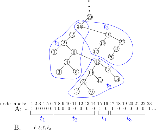
Figure 1: Figure depicts a part of a binary tree where $t_{1}$, $t_{2}$, and $t_{3}$ are its three mini-trees. Node labels are in inorder ordering of these nodes. Each node has a corresponding bit in $A$ and each mini-tree has one or two corresponding labels ($\ell_{i}$ is the label of $t_{i}$) in $B$.

We observe that a node $v$ with inorder number $i$ belongs to the mini-tree with rank $B[\text{rank}_{A}(1,i+1)]$, and thus $P[B[\text{rank}_{A}(1,i+1)]]$ contains the preorder number of the root of the mini-tree containing $v$.

We represent $A$ using the data structure of Lemma 2, which supports rank in constant time. In order to analyze the space, we prove that the number of $1$s in $A$ is at most $2n_{m}$: each mini-tree has at most one edge leaving the mini-tree aside from its root, which means that the traversal can enter or re-enter a mini-tree at most twice. Therefore, the space usage is $\lg{n\choose 2n_{m}}+o(n)=o(n)$ bits, as $n_{m}=O(n/\log^{2}n)$. We store $P$ and $B$ explicitly with no preprocessing on them. The length of $B$ is also at most $2n_{m}$ by the same argument. Thus, both $P$ and $B$ take $O(n/\log^{2}n\cdot\log n)=o(n)$ bits.

(2) Let $S$ be the set of nodes that are visited after $r_{m}$ and before $v$ in the preorder traversal of the tree. Notice that $c(v,r_{m})=|S|$. Let $t_{m}$ and $t_{\mu}$ be respectively the mini-tree and micro-tree containing $v$. We note that $S=S_{1}\cup S_{2}\cup S_{3}$, where $S_{1}$ contains the nodes of $S$ that are not in $t_{m}$, $S_{2}$ contains the nodes of $S$ that are in $t_{\mu}$, and $S_{3}$ contains the nodes that are in $t_{m}$ and not in $t_{\mu}$. Observe that $S_{1}$, $S_{2}$, and $S_{3}$ are mutually disjoint. Therefore, $c(v,r_{m})=|S_{1}|+|S_{2}|+|S_{3}|$. We now describe how to compute each size.

$S_{1}$: If $t_{m}$ has a boundary node which is visited before the root of $t_{\mu}$, then $|S_{1}|$ is the subtree size of the child of the boundary node that is out of $t_{m}$; otherwise $|S_{1}|=0$.

$S_{2}$: Since these nodes are within a micro-tree, $|S_{2}|$ can be computed using a lookup-table.

$S_{3}$: The local preorder number of the root of $t_{\mu}$, which results from traversing $t_{m}$ while ignoring the edges leaving $t_{m}$, is equal to $|S_{3}|$. We precompute the local preorder numbers of all the micro-tree roots. The method to store these local preorder numbers and the data structure that we construct in order to efficiently retrieve these numbers is similar to the part (1), whereas here a mini-tree plays the role of the input tree and micro-trees play the role of the mini-trees. In other words, we construct $P$, $A$, and $B$ of part (1) for each mini-tree. The space usage of this data structure is $o(n)$ bits by the same argument, regarding the fact that each local preorder number takes $O(\log\log n)$ bits.

Theorem 1.

A binary tree with $n$ nodes can be represented with a succinct data structure of size $2n+o(n)$ bits, which supports node-rank${}_{\text{inorder}}$, node-select${}_{\text{inorder}}$, plus a comprehensive set of operations (fm-algo12, , Table 2), all in $O(1)$ time.

2.3 RMQs on Random Inputs

The following theorem gives a slight generalization of Theorem 1, which uses entropy coding to exploit any differences in frequency between different types of nodes (Theorem 1 corresponds to choosing all the $\alpha_{i}$s to be $1/4$ in the following):

Theorem 2.

For any positive constants $\alpha_{0},\alpha_{L},\alpha_{R}$ and $\alpha_{2}$, such that $\alpha_{0}+\alpha_{L}+\alpha_{R}+\alpha_{2}=1$, a binary tree with $n_{0}$ leaves, $n_{L}$ ($n_{R}$) nodes with only a left (right) child and $n_{2}$ nodes with both children can be represented using $\left(\sum_{i\in\{0,L,R,2\}}n_{i}\lg(1/\alpha_{i})\right)+o(n)$ bits of space, while a full set of operations (fm-algo12, , Table 2) including node-rank${}_{\text{inorder}}$, node-select${}_{\text{inorder}}$ and LCA can be supported in $O(1)$ time.

Proof.

We proceed as in the proof of Theorem 1, but if $\alpha=\min_{i\in\{0,L,R,2\}}\alpha_{i}$, we choose the size of the micro-trees to be at most $\mu=\frac{\lg n}{2\lg(1/\alpha)}=\Theta(\log n)$. The $2n$-bit term in the representation of fm-algo12 comes from the representation of the microtrees. Given a micro-tree with $\mu_{i}$ nodes of type $i$, for $i\in\{0,L,R,2\}$ we encode it by writing the node types in level order (cf. jacobson89 ) and encoding this string using arithmetic coding with the probability of a node of type $i$ taken to be $\alpha_{i}$. The size of this encoding is at most  $\left(\sum_{i\in\{0,L,R,2\}}\mu_{i}\lg(1/\alpha_{i})\right)+2$ bits, from which the theorem follows. Note that our choice of $\mu$ guarantees that each microtree fits in $\frac{\lg n}{2}$ bits and thus can still be manipulated using universal look-up tables. ∎

Corollary 1.

If $A$ is a random permutation over $\{1,\ldots,n\}$, then RMQ queries on $A$ can be answered using $(\frac{1}{3}+\lg 3)n+o(n)<1.919n+o(n)$ bits in expectation.

Proof.

Choose $\alpha_{0}=\alpha_{2}=1/3$ and $\alpha_{R}=\alpha_{L}=1/6$. The claim follows from the fact that $\alpha_{i}n$ is the average value of $n_{i}$ on random binary trees, for any $i\in\{0,L,R,2\}$ (gikrs-isaac11, , Theorem 1). ∎

While both our representation and that of Fischer and Heun fh-sjc11 solve RMQs in $O(1)$ time and use $2n+o(n)$ bits in the worst case, ours allows an improvement in the average case. However, we are unable to match the expected effective entropy of RMQs on random arrays $A$, which is $\approx 1.736n+O(\log n)$ bits (GIKRRS12, , Thm. 1) (see also Kieffer2009 ).

It is natural to ask whether one can obtain improvements for the average case via Fischer and Heun’s approach fh-sjc11 as well. Their approach first converts the Cartesian tree to an ordinal tree (an ordered, rooted tree) using the textbook transformation CLR . To the best of our knowledge, the only ordinal tree representation able to use $(2-\Theta(1))n$ bits is the so-called ultra-succinct representation JSS07 , which uses $\sum_{a}n_{a}\lg\frac{n}{n_{a}}+o(n)$ bits, where $n_{a}$ is the number of nodes with $a$ children. Our empirical simulations suggest that the combination of fh-sjc11 with JSS07 would not use $(2-\Omega(1))n$ bits on average on random permutations. We generated random permutations of sizes $10^{3}$ to $10^{7}$ and measured the entropy $\sum_{a}n_{a}\lg\frac{n}{n_{a}}$ on the resulting Cartesian trees. The results, averaged over 100 to 1,000 iterations, are $1.991916$, $1.998986$, $1.999869$, $1.999984$ and $1.999998$, respectively. The results appear as a straight line on a log-log plot, which suggests a formula of the form $2n-f(n)$ for a very slowly growing function $f(n)$. Indeed, using the model $2n-O(\log n)$ we obtain the approximation $2n-0.81\lg n$ with a mean squared error below $10^{-9}$.

To understand the observed behaviour, first note that when the Cartesian tree is converted to an ordinal tree, the arity of each ordinal tree node $u$ turns out to be, in the Cartesian tree, the length of the path from the right child $v$ of $u$ to the leftmost descendant of $u$ (i.e., the node representing $u+1$ if we identify Cartesian tree nodes with their positions in $A$). This is called $r_{u}$ (or $L_{v}$) in the next section. Next, note that:

Fact 1.

The probability that a node $v$ of the Cartesian tree of a random permutation has a left child is $\frac{1}{2}$.

Proof.

Consider the values $A[v-1]$ and $A[v]$. If $A[v]<A[v-1]$, then $\text{RMQ}(v-1,v)=v=\text{LCA}(v-1,v)$, thus $v-1$ descends from $v$ and hence $v$ has a left child. If $A[v]>A[v-1]$, then $\text{RMQ}(v-1,v)=v-1=\text{LCA}(v-1,v)$, thus $v$ descends from $v-1$ and hence $v$ is the leftmost node of the right subtree of $v-1$, and therefore $v$ cannot have a left child. Therefore $v$ has a left child iff $A[v]<A[v-1]$, which happens with probability $\frac{1}{2}$ in a random permutation. ∎

Thus, if we disregarded the dependencies between nodes in the tree, we could regard $L_{v}$ as a geometric variable with parameter $\frac{1}{2}$, and thus the expected value of $n_{a}$ would be $\mathbb{E}(n_{a})=\frac{n}{2^{a+1}}$. Taking the expectation as a fixed value, the space would be $\sum_{a}\mathbb{E}(n_{a})\lg\frac{n}{\mathbb{E}(n_{a})}=\sum_{a\geq 0}\frac{n(a+1)}{2^{a+1}}=2n$. Although this is only a heuristic argument (as we are ignoring both the dependencies between tree nodes and the variance of the random variables), our empirical results nevertheless suggest that this simplified model is asymptotically accurate, and thus, that no space advantage is obtained by representing random Cartesian trees, as opposed to worst-case Cartesian trees, using this scheme.

3 Range Top-2 Queries

In this section we consider a generalization of the RMQ problem. Again, let $A[1..n]$ be an array of elements from a totally ordered set. Let $\text{R2M}(i,j)$, for any $1\leq i<j\leq n$, denote the position of the second smallest value in $A[i..j]$. More formally:

$$\text{R2M}(i,j)=\text{argmin}\{A[k]:{k\in([i..j]\setminus\text{RMQ}(i,j))}\}\;.$$

The encoding RT2Q problem is to preprocess $A$ into a data structure that, given $i,j$, returns $\text{RT2Q}(i,j)=(\text{RMQ}(i,j),\text{R2M}(i,j))$, without accessing $A$ at query time.

The idea is to augment the Cartesian tree of $A$, denoted $T_{A}$, with some information that allows us to answer $\text{R2M}(i,j)$. If $h$ is the position of the minimum element in $A[i..j]$ (i.e., $h=\text{RMQ}(i,j)$), then $h$ divides $[i..j]$ into two subranges $[i..h-1]$ and $[h+1..j]$, and the second minimum is the smaller of the elements $A[\text{RMQ}(i,h-1)]$ and $A[\text{RMQ}(h+1,j)]$. Except for the case where one of the subranges is empty, the answer to this comparison is not encoded in $T_{A}$. We describe how to succinctly encode the ordering between the elements of $A$ that are candidates for $\text{R2M}(i,j)$. Our data structure consists of this encoding together with the encoding of $T_{A}$ using the representation of Theorem 1 (along with the operations mentioned in Section 2).

We define the left spine of a node $u$ to be the set of nodes on the downward path from $u$ (inclusive) that follows left children until this can be done no further. The right spine of a node is defined analogously. The left inner spine of a node $u$ is the right spine of $u$’s left child. If $u$ does not have a left child then it has an empty left inner spine. The right inner spine is defined analogously. We use the notation $\text{lspine}(v)$/$\text{rspine}(v)$, $\text{lispine}(v)$/$\text{rispine}(v)$, $L_{v}/R_{v}$ and $l_{v}/r_{v}$ to denote the left/right spines of $v$, the left/right inner spines of $v$, and the number of nodes in the spines and inner spines of $v$ respectively. We also assume that nodes are numbered in inorder and identify node names with their inorder numbers.

As previously mentioned, our data structure encodes the ordering between the candidates for $\text{R2M}(i,j)$. We first identify locations for these candidates:

Lemma 4.

In $T_{A}$, for any $i,j\in[1..n]$, $i<j$, $\text{R2M}(i,j)$ is located in $\text{lispine}(v)$ or $\text{rispine}(v)$, where $v=\text{RMQ}(i,j)$.

Proof.

Let $v=\text{RMQ}(i,j)$. The second minimum clearly lies in one of two subranges $[i..v-1]$ and $[v+1..j]$, and it must be equal to either $\text{RMQ}(i,v-1)$ or $\text{RMQ}(v+1,j)$. W.l.o.g. assume that $[i..v-1]$ is non-empty: in this case the node $v-1$ is the bottom-most node on $\text{lispine}(v)$. Furthermore, since $v=\text{RMQ}(i,j)$, $i$ must lie in the left subtree of $v$. Since the LCA of the bottom-most node on $\text{lispine}(v)$ and any other node in the left subtree of $v$ is a node in $\text{lispine}(v)$, $\text{RMQ}(i,v-1)$ is in $\text{lispine}(v)$. The analogous statement holds for $\text{rispine}(v)$. ∎

Thus, for any node $v$, it suffices to store the relative order between nodes in $\text{lispine}(v)$ and $\text{rispine}(v)$ to find $\text{R2M}(i,j)$ for all queries for which $v$ is the answer to the RMQ query. As $T_{A}$ determines the ordering among the nodes of $\text{lispine}(v)$ and also among the nodes of $\text{rispine}(v)$, we only need to store the information needed to merge $\text{lispine}(v)$ and $\text{rispine}(v)$. We will do this by storing $m_{v}=\max(l_{v}+r_{v}-1,0)$ bits associated with $v$, for all nodes $v$, as explained later. We need to bound the total space required for the ‘merging’ bits, as well as to space-efficiently realize the association of $v$ with the the $m_{v}$ merging bits associated with it. For this, we need the following auxiliary lemmas:

Lemma 5.

Let $T$ be a binary tree with $m$ nodes (of which $m_{0}$ are leaves) and root $u$. Then, $\sum_{v\in T}(l_{v}+r_{v})=2m-L_{u}-R_{u}$, and $\sum_{v\in T}m_{v}\leq m-L_{u}-R_{u}+m_{0}$.

Proof.

The first part follows from the fact that the $R_{u}$ nodes in $\text{rspine}(u)$ do not appear in $\text{lispine}(v)$ for any $v\in T$, and all the other nodes in $T$ appear exactly once in a left inner spine. Similarly, the $L_{u}$ nodes in $\text{lspine}(u)$ do not appear in $\text{rispine}(v)$ for any $v\in T$, and the other nodes in $T$ appear exactly once in a right inner spine. Then the second part follows from the fact that $m_{v}=l_{v}+r_{v}-1$ iff $l_{v}+r_{v}>0$, that is, $v$ is not a leaf. If $v$ is a leaf, then $l_{v}+r_{v}=0=m_{v}$. Thus we must subtract $m-m_{0}$ from the previous formula, which is the number of non-leaf nodes in $T$. ∎

In the following lemma, we utilize two operations $\text{Ldepth}(v)$ and $\text{Rdepth}(v)$ which compute the number of nodes that have their left and right child, respectively, in the path from root to $v$ (recall that $\text{Ldepth}(v)$ computes $c_{2}(v)$ defined in Section 2).

Lemma 6.

Let $T$ be a binary tree with $m$ nodes and root $\tau$. Suppose that the nodes of $T$ are numbered $0,\ldots,m-1$ in inorder. Then, for any $0\leq u<m$:

$$\sum_{j<u}(l_{j}+r_{j})=2u-L_{\tau}-l_{u}+\text{Ldepth}(u)-\text{Rdepth}(u)+1.$$

Proof.

The proof is by induction on $m$. For the base case $m=1$, $\tau=u=0$ is the only possibility and the formula evaluates to 0 as expected: $l_{u}=\text{Ldepth}(u)=\text{Rdepth}(u)=0$ and $L_{\tau}=1$ (recall that $\tau$ is included in $\text{lspine}(\tau)$).

Now consider a tree $T$ with root $\tau$ and $m>1$ nodes. We consider the three cases $u=\tau$, $u<\tau$ and $u>\tau$ in that order. If $u=\tau$ then $\text{Ldepth}(\tau)=\text{Rdepth}(\tau)=0$. If $\tau$ has no left child, the situation is the same as when $m=1$. Else, letting $v$ be the left child of $\tau$, note that $L_{v}=L_{\tau}-1$ and since $\text{lispine}(\tau)=\text{rspine}(v)$, $l_{\tau}=R_{v}$. As the subtree rooted at $v$ has size exactly $\tau$, the formula can be rewritten as $2\tau-L_{v}-R_{v}$, its correctness follows from Lemma 5 without recourse to the inductive hypothesis.

If $u<\tau$ then by induction on the subtree rooted at the left child $v$ of $\tau$, the formula gives $2u-L_{v}-l_{u}+\text{Ldepth}^{\prime}(u)-\text{Rdepth}^{\prime}(u)+1$, where $\text{Rdepth}^{\prime}$ and $\text{Ldepth}^{\prime}$ are measured with respect to $v$. As $\text{Ldepth}^{\prime}(u)=\text{Ldepth}(u)-1$, $\text{Rdepth}^{\prime}(u)=\text{Rdepth}(u)$ and $L_{v}=L_{\tau}-1$, this equals $2u-L_{\tau}-l_{u}+\text{Ldepth}(u)-\text{Rdepth}(u)+1$ as required.

Finally we consider the case $u>\tau$. Letting $v$ and $w$ be the left and right children of $\tau$, and $u^{\prime}=u-\tau-1$, we note that $u^{\prime}$ is the inorder number of $u$ in the subtree rooted at $w$. Applying the induction hypothesis to the subtree rooted at $w$, we get that:

$$\sum_{\tau<j<u}(l_{j}+r_{j})=2u^{\prime}-L_{w}-l_{u}+\text{Ldepth}^{\prime}(u)-\text{Rdepth}^{\prime}(u)+1,$$

where $\text{Rdepth}^{\prime}$ and $\text{Ldepth}^{\prime}$ are measured with respect to $w$. Simplifying:

$$\sum_{j<u}(l_{j}+r_{j})~{}~{}=~{}~{}\sum_{j<\tau}(l_{j}+r_{j})+l_{\tau}+r_{\tau}+\sum_{\tau<j<u}(l_{j}+r_{j})$$

$$= 2\tau-L_{v}-R_{v}+l_{\tau}+r_{\tau}+2u^{\prime}-L_{w}-l_{u}+\text{Ldepth}^{\prime}(u)-\text{Rdepth}^{\prime}(u)+1$$

$$= 2\tau-L_{v}-R_{v}+l_{\tau}+r_{\tau}+2u^{\prime}-L_{w}-l_{u}+\text{Ldepth}(u)-\text{Rdepth}(u)+2$$

$$= 2\tau-L_{v}+2u^{\prime}-l_{u}+\text{Ldepth}(u)-\text{Rdepth}(u)+2$$

$$= 2\tau-(L_{\tau}-1)+2(u-\tau-1)-l_{u}+\text{Ldepth}(u)-\text{Rdepth}(u)+2$$

$$= 2u-L_{\tau}-l_{u}+\text{Ldepth}(u)-\text{Rdepth}(u)+1$$

Here we have made use (in order) of Lemma 5 and the facts $\text{Ldepth}^{\prime}(u)=\text{Ldepth}(u)$ and $\text{Rdepth}^{\prime}(u)=\text{Rdepth}(u)-1$; $L_{w}=r_{\tau}$ and $R_{v}=l_{\tau}$; and finally $L_{v}=L_{\tau}-1$. ∎

Corollary 2.

In the same scenario of Lemma 6, we have

$$\sum_{j<u}m_{j}~{}=~{}2u-L_{\tau}-l_{u}+\text{Ldepth}(u)-\text{Rdepth}(u)+1-\text{Lleaves}(u),$$

where $\text{Lleaves}(u)$ is the number of leaves to the left of node $u$.

Proof.

Trivially follows from Lemma 6 and the same considerations as in the proof of Lemma 5. ∎

The Data Structure.

For each node $u$ in $T_{A}$, we create a bit sequence $M_{u}$ of length $m_{u}$ to encode the merge order of $\text{lispine}(u)$ and $\text{rispine}(u)$. $M_{u}$ is obtained by taking the sequence of all the elements of $\text{lispine}(u)\cup\text{rispine}(u)$ sorted in decreasing order, and replacing each element of this sorted sequence by 0 if the element comes from $\text{lispine}(u)$ and by 1 if the element comes from $\text{rispine}(u)$ (the last bit is omitted, as it is unnecessary). We concatenate the bit sequences $M_{u}$ for all $u\in T_{A}$ considered in inorder and call the concatenated sequence $M$.

The data structure comprises $M$, augmented with $rank$ and $select$ operations and a data structure for $T_{A}$. If we use Theorem 1, then $T_{A}$ is represented in $2n+o(n)$ bits, and the (augmented) $M$ takes at most $1.5n+o(n)$ bits by Lemmas 5 and 1, since there are at most $(n+1)/2$ leaves in an $n$-node binary tree. This gives a representation whose space is $3.5n+o(n)$ bits. A further improvement can be obtained by using Theorem 2 as follows. For some real parameter $0<x<1$, consider the concave function:

$$H(x)~{}~{}=~{}~{}2x\lg\frac{1}{x}+2\frac{(1-2x)}{2}\lg\frac{2}{1-2x}+x+1.$$

Differentiating and simplifying, we get the maximum of $H(x)$ as the solution to the equation $2(\lg(1-2x)-\lg x)=1$, from which we get that $H(x)$ is maximized at $x=1-\sqrt{2}/2\approx 0.293$, and attains a maximum value of $\gamma=2+\lg(1+\sqrt{2})<3.272$.

Now let $n_{0},n_{L}(n_{R})$ and $n_{2}$ be the numbers of leaves, nodes with only a left (right) child and nodes with both children in $T_{A}$. Letting $x=n_{0}/n$, we apply Theorem 2 to represent $T_{A}$, using the parameters $\alpha_{0}=\alpha_{2}$ to be equal to $x$, but capped to a minimum of $0.05$ and a maximum of $0.45$, i.e. $\alpha_{0}=\alpha_{2}=\max\{\min\{0.45,x\},0.05\}$, and $\alpha_{L}=\alpha_{R}=(1-2\alpha_{0})/2$. Observe that the capping means that $\alpha_{L}$ and $\alpha_{R}$ lie in the range $[0.05,0.45]$ as well, thus satisfying the condition in Theorem 2 requiring the $\alpha_{i}$’s to be constant. Then the space used by the representation is $\left(\sum_{i\in\{0,L,R,2\}}n_{i}\lg(1/\alpha_{i})\right)+n+n_{0}+o(n)$ bits. Provided capping is not applied, and since $n_{0}=n_{2}+1$ and $\alpha_{L}=\alpha_{R}$, this is easily seen to be $nH(x)+o(n)$ bits, and is therefore bounded by $\gamma n+o(n)$ bits. If $x>0.45$, then the representation takes $2n_{0}\lg(1/0.45)+(n-2n_{0})\lg(1/0.05)+n+n_{0}+o(n)$ bits. Since $2\lg(1/0.45)-2\lg(1/0.05)+1<0$, this is maximized with the least possible $n_{0}=0.45n$, where the space is precisely $nH(0.45)+o(n)<\gamma n+o(n)$. Similarly, for $x<0.05$ the space is less than $nH(0.05)+o(n)<\gamma n+o(n)$ bits.

We now explain how this data structure can answer RT2Q in constant time. We utilize the data structure of Theorem 2 constructed on $T_{A}$ in order to find $u=\text{LCA}({i},{j})=\text{RMQ}(i,j)$. Subsequently:

1. We determine the start of $M_{u}$ within $M$ by calculating $\sum_{j<u}m_{j}$.

2. We locate the appropriate nodes from $\text{lispine}(u)$ and $\text{rispine}(u)$ and the corresponding bits within $M_{u}$ and make the required comparison.

We now explain each of these steps. For step (1), we use Corollary 2. When evaluating the formula, we use the $O(1)$-time support for $\text{Ldepth}(u)$ and $\text{Rdepth}(u)$ given by the data structure of Section 2; there we explain $\text{Ldepth}(u)$ indeed computes $c_{2}(u)$ and we describe how to compute $c_{2}(u)$ in constant time (computing $\text{Rdepth}(u)$ can be done analogously). This leaves only the computation of $l_{u}$ and $\text{Lleaves}(u)$. The former is done as follows. We check if $u$ has a left child: if not, then $l_{u}=0$. Otherwise, if $v$ is $u$’s left child, then $v$ and $u-1$ are respectively the topmost and lowest nodes in $\text{lispine}(u)$. We can then obtain $l_{u}$ in $O(1)$ time as $\text{depth}(v)-\text{depth}(u)$ in $O(1)$ time by Theorem 2. On the other hand, $\text{Lleaves}(u)$ can be computed as $\text{leaf-rank}(v^{\prime}+\text{subtree-size}(v^{\prime})-1)$, where $v^{\prime}=\text{node-select}_{\mathrm{inorder}}(v)$ and $v$ is the left child of $u$. If $v$ does not exist then $\text{Lleaves}(u)=\text{leaf-rank}(u^{\prime})$, where $u^{\prime}=\text{node-select}_{\mathrm{inorder}}(u)$. All those operations take $O(1)$ time by Theorem 2.

For step (2) we use Lemma 4 to locate the two candidates from $A[i..u-1]$ and $A[u+1..j]$ (assuming that $i<u<j$, if not, the problem is easier) in $O(1)$ time as $v=\text{LCA}(i,u-1)$ and $w=\text{LCA}(u+1,j)$. Next we obtain the rank $\rho_{v}$ of $v$ in $\text{lispine}(u)$ in $O(1)$ time as $\text{depth}(u-1)-\text{depth}(v)$. The rank $\rho_{w}$ of $w$ in $\text{rispine}(u)$ is obtained similarly. Now, letting $\Delta=\sum_{j<u}(l_{j}+r_{j})$, we compare $\text{select}_{M}(0,\text{rank}_{M}(0,\Delta)+\rho_{v})$ and $\text{select}_{M}(1,\text{rank}_{M}(1,\Delta)+\rho_{w})$ in $O(1)$ time to determine which of $v$ and $w$ is smaller and return that as the answer to $\text{R2M}(i,j)$. We have thus shown:

Theorem 3.

Given an array of $n$ elements from a totally ordered set, there exists a data structure of size at most $\gamma n+o(n)$ bits that supports RT2Qs in $O(1)$ time, where $\gamma=2+\lg(1+\sqrt{2})<3.272$.

Note that $\gamma n$ is a worst-case bound. The size of the encoding can be less for other values of $n_{0}$. In particular, since $H(x)$ is convex and the average value of $n_{0}$ on random permutations is $n/3$ (gikrs-isaac11, , Theorem 1), we have by Jensen’s inequality that the expected size of the encoding is below $H(1/3)=\lg(3)+\frac{5}{3}<3.252$.

4 Effective Entropy of RT2Q and R2M

In this section we lower bound the effective entropy of RT2Q, that is, the number of equivalence classes $\mathcal{C}$ of arrays distinguishable by RT2Qs. For this sake, we define extended Cartesian trees, in which each node $v$ indicates a merging order between its left and right internal spines, using a number in a universe of size ${l_{v}+r_{v}\choose r_{v}}$. We prove that any distict extended Cartesian tree can arise for some input array, and that any two distinct extended Cartesian trees give a different answer for at least some RT2Q. Then we aim to count the number of distinct extended Cartesian trees.

While unable to count the exact number of extended Cartesian trees, we provide a lower bound by unrolling their recurrence a finite number of times (precisely, up to 7 levels). This effectively limits the lengths of internal spines we analyze, and gives us a number of configurations of the form $\frac{1}{0.160646^{n}}\,\theta(n)$ for a polynomial $\theta(n)$, from where we obtain a lower bound of $2.638n-O(\log n)$ bits on the effective entropy of RT2Q.

We note that our bound on RT2Qs also applies to the weaker R2M operation, since any encoding answering R2Ms has enough information to answer RT2Qs. Indeed, it is easy to see that RMQ$(i,j)$ is the only position that is not the answer of any query R2M$(i^{\prime},j^{\prime})$ for any $i\leq i^{\prime}<j^{\prime}\leq j$. Then, with RMQ and R2M, we have RT2Q. Therefore we can give our result in terms of the weaker R2M.

Theorem 4.

The effective entropy of R2M (and RT2Q) over an array $A[1,n]$ is at least $2.638n-O(\log n)$.

4.1 Modeling the Effective Entropy of R2M

Recall that to show that the effective entropy of RMQ is $2n-O(\log n)$ bits, we argue that $(i)$ any two Cartesian trees will give a different answer to at least one $\text{RMQ}(i,j)$; $(ii)$ any binary tree is the Cartesian tree of some permutation $A[1,n]$; $(iii)$ the number of binary trees of $n$ nodes is $\frac{1}{n+1}{2n\choose n}$, thus in the worst case one needs at least $\lg\left(\frac{1}{n+1}{2n\choose n}\right)=2n-O(\log n)$ bits to distinguish among them.

A similar reasoning can be used to establish a lower bound on the effective entropy of RT2Q. We consider an extended Cartesian tree $T$ of size $n$, where for any node $v$ having both left and right children we store a number $M(v)$ in the range $[1..{l_{v}+r_{v}\choose r_{v}}]$. The number $M(v)$ identifies one particular merging order between the nodes in lispine$(v)$ and rispine$(v)$, and ${l_{v}+r_{v}\choose r_{v}}$ is the exact number of different merging orders we can have.

Now we follow the same steps as before. For $(i)$, let $T$ and $T^{\prime}$ be Cartesian trees extended with the corresponding numbers $M(v)$ for $v\in T$ and $M^{\prime}(v^{\prime})$ for $v^{\prime}\in T^{\prime}$. We already know that if the topologies of $T$ and $T^{\prime}$ differ, then there exists an $\text{RMQ}(i,j)$ that gives different results on $T$ and $T^{\prime}$. Assume now that the topologies are equal, but there exists some node $v$ where $M(v)$ differs from $M^{\prime}(v)$. Then there exists an $\text{RT2Q}(i,j)$ where the extended trees give a different result. W.l.o.g., let $i$ and $j$ be the first positions of lispine$(v)$ and rispine$(v)$, respectively, where $v_{l}=\textrm{lispine}(v)[i]$ goes before $v_{r}=\textrm{rispine}(v)[j]$ according to $M(v)$, but after according to $M^{\prime}(v)$. Then $T$ answers $\text{R2M}(v_{1},v_{2})=v_{1}$ and $T^{\prime}$ answers $\text{R2M}(v_{1},v_{2})=v_{2}$ (we interpret $v_{1}$ and $v_{2}$ as inorder numbers here).

As for $(ii)$, let $T$ be an extended Cartesian tree, where $u$ is the (inorder number of the) root of $T$. Then we build a permutation $A[1,n]$ whose extended tree is $T$ as follows. First, we set the minimum at $A[u]=0$. Now, we recursively build the ranges $A[1,u-1]$ (a permutation in with values in $[0..u-1]$) and $A[u+1,n]$ (a permutation with values in $[0..n-u-1]$) for the left and right child of $T$, respectively. Assume, inductively, that the permutations already satisfy the ordering given by the $M(v)$ numbers for all the nodes $v$ within the left and right children of $u$. Now we are free to map the values of $A\setminus A[u]$ to the interval $[1,n-1]$ in any way that maintains the relative ordering within $A[1,u-1]$ and $A[u+1,n]$. We do so in such a way that the elements of lispine$(u)$ and rispine$(u)$ compare according to $M(u)$. This is always possible: We sort $A[1,u-1]$ and $A[u+1,n]$ from smallest to largest values, let $A[a_{i}]$ be the $i$th smallest cell of $A[1,u-1]$ and $A[b_{j}]$ the $i$th smallest cell of $A[u+1,n]$. Also, we set cursors at lispine$(u)[l]$ and rispine$(u)[r]$, initially $l=r=1$, and set $c=i=j=1$. At each step, if $M(u)$ indicates that lispine$(u)[l]$ comes before rispine$(u)[r]$, we reassign $A[a_{i}]=c$ and increase $i$ and $c$, until (and including) the reassignment of $a_{i}=\textrm{lispine}(u)[l]$, then we increase $l$; otherwise we reassign $A[b_{j}]=c$ and increase $j$ and $c$, until (and including) the reassignment of $b_{j}=\textrm{rispine}(u)[r]$, then we increase $r$. We repeat the process until reassigning all the values in $A\setminus A[u]$.

For $(iii)$, next we will lower bound the total number of extended Cartesian trees.

4.2 Lower Bound on Effective Entropy

As explained, we have been unable to come up with a general counting for the lower bound, yet we give a method that can be extended with more and more effort to reach higher and higher lower limits. The idea is to distinguish the first steps in the generation of the Cartesian tree out of the root node, and charge the minimum value of ${l_{v}+r_{v}\choose r_{v}}$ we can ensure in each case. Let

$$T(x)~{}~{}=~{}~{}\sum_{n>0}t(n)x^{n}$$

where $t(n)$ is the number of extended Cartesian trees with $n$ nodes, counted using some simple lower-bounding technique. For example, if we consider the simplest model for $T(x)$, we have that a (nonempty) tree is a root $v$ either with no children, with a left child rooting a tree, with a right child rooting a tree, or with left and right children rooting trees, this time multiplied by 2 to account for ${l_{v}+r_{v}\choose r_{v}}\geq{2\choose 1}$ (see the levels 0 and 1 in Figure 2). Then $T(x)$ satisfies

$$T(x)~{}~{}=~{}~{}x+xT(x)+xT(x)+2xT(x)^{2}~{}~{}=~{}~{}x+2xT(x)+2xT(x)^{2},$$

which solves to

$$T(x)~{}~{}=~{}~{}\frac{1-2x-\sqrt{1-4x-4x^{2}}}{4x},$$

which has two singularities at $x=\frac{-1\pm\sqrt{2}}{2}$. The one closest to the origin is $x=\frac{\sqrt{2}-1}{2}$. Thus it follows that $t(n)$ is of the form $\left(\frac{2}{\sqrt{2}-1}\right)^{n}\theta(n)$ for some polynomial $\theta(n)$ SF95 , and thus we need at least $\lg\left(\left(\frac{2}{\sqrt{2}-1}\right)^{n}\theta(n)\right)=\lg\left(\frac{2}{\sqrt{2}-1}\right)n-O(\log n)\geq 2.271n-O(\log n)$ bits to represent all the possible extended Cartesian trees.

Figure 2: Our scheme to enumerate extended Cartesian trees $T$ with increasing detail, where the $x$ stands for a node and $T$ for any subtree. We indicate the numbers ${l_{v}+r_{v}\choose r_{v}}$ below nodes having left and right internal spines. Level 0 corresponds just to $T(x)$. In level 1 we have four possibilities, which lead to the equation $T(x)=x+2xT(x)+2xT(x)^{2}$. For level 2, each of the $T$s in level 1 is expanded in all the four possible ways, leading to 25 possibilities and to the equation $T(x)=x+2x^{2}+4x^{2}T(x)+4x^{2}T(x)^{2}+2x^{3}+10x^{3}T(x)+26x^{3}T(x)^{2}+36x^{3}T(x)^{3}+24x^{3}T(x)^{4}$.

This result can be improved by unrolling the recurrence of $T$ further, that is, replacing each $T$ by its four possible alternatives in the basic definition. Then the lower bound improves because some left and right internal spines can be seen to have length two or more. The results do not admit easy algebraic solutions anymore, but we can numerically analyze the resulting functions with Maple and establish a safe numeric threshold from where higher lower bounds can be derived. For example by doing a first level of replacement in the simple recurrence, we obtain a recurrence with 25 cases, which yields

$$T(x)~{}=~{}x+2x^{2}+4x^{2}T(x)+4x^{2}T(x)^{2}+2x^{3}+10x^{3}T(x)+26x^{3}T(x)^{2}+36x^{3}T(x)^{3}+24x^{3}T(x)^{4};$$

(see level 2 in Figure 2) which Maple is able to solve algebraically, although the formula is too long to display it here. While Maple could not algebraically find the singularities of $T(x)$, we analyzed the result numerically and found a singularity at $x=0.190879...$ Therefore, we conclude that $t(n)\geq\frac{1}{0.190880^{n}}\theta(n)$, and thus that a lower bound is $n\,\lg\frac{1}{0.190880}-O(\log n)\geq 2.389n-O(\log n)$.

To find the singularity we used the result (SF09, , Thm. VII.3) that, under certain conditions that are met in our case, the singularities of an equation of the form $T(x)=G(x,T(x))$ can be found by numerically solving the system formed by the equation $T=G(x,T)$ and its derivative, $1=\frac{\partial G(x,T)}{\partial T}$. If the positive solution is found at $(x=r,T=\gamma)$, then there is a singularity at $x=r$. If, further, $T(x)$ is aperiodic (as in our case), then $r$ is the unique dominant singularity and $t(n)=\frac{1}{r^{n}}\,\theta(n)$ for some polynomial $\theta(n)$.

To carry the idea further, we wrote a program that generates all the combinations of any desired level, and builds a recurrence to feed Maple with. We use the program to generate the recurrences of level 3 onwards. Table 1 shows the results obtained up to level 7, which is the one yielding the lower bound $2.638n-O(\log n)$ of Theorem 4. This was not without challenges; we describe the details in the Appendix.

Level	# of cases	# of terms	degree	singularity	lower bound
1	4	3	2	0.207107	$2.271n-O(\log n)$
2	25	9	4	0.190879	$2.389n-O(\log n)$
3	675	63	8	0.179836	$2.474n-O(\log n)$
4	$\sim 4.6\times 10^{5}$	119	16	0.172288	$2.537n-O(\log n)$
5	$\sim 2.1\times 10^{11}$	479	32	0.167053	$2.581n-O(\log n)$
6	$\sim 4.4\times 10^{22}$	1951	64	0.163343	$2.621n-O(\log n)$
7	$\sim 1.9\times 10^{45}$	7935	128	0.160646	$2.638n-O(\log n)$

Table 1: Our results for increasing number of levels. The second column gives the number of cases generated, the third the number of terms in the resulting polynomial, the fourth the degree of the polynomial in $x$ and $T$, the fifth the $x$ value of the singularity found, and the last column gives the implied lower bound.

5 Conclusions

We obtained a succinct binary tree representation that extends the representation of Farzan and Munro fm-algo12 by supporting navigation based on the inorder numbering of the nodes, and a few additional operations. Using this representation, we describe how to encode an array in optimal space in a more natural way than the existing structures, to support RMQs in constant time. In addition, this representation reaches $1.919n+o(n)$ bits on random permutations, thus breaking the worst-case lower bound of $2n-O(\log n)$ bits. This is not known to hold on any alternative representation. It is an open question to find a data structure that answers RMQs in $O(1)$ time using $2n+o(n)$ bits in the worst case, while also achieving the expected effective entropy bound of about $1.736n$ bits for random arrays $A$.

Then, we obtain another structure that encodes an array of $n$ elements from a total order using $3.272n+o(n)$ bits to support RT2Qs in $O(1)$ time. This uses almost half of the $6n+o(n)$ bits used for this problem in the literature GINRS13 . Our structure can possibly be plugged in their solution, thus reducing their space.

While the effective entropy of RMQs is known to be precisely $2n-O(\log n)$ bits, the effective entropy for range top-$k$ queries is only known asymptotically: it is at least $n\lg k-O(n)$ bits, and at most $O(n\log k)$ bits GINRS13 . We have shown that, for $k=2$, the effective entropy is at least $2.638n-O(\log n)$ bits. Determining the precise effective entropy for $k\geq 2$ is an open question.

Appendix A Unrolling the Lower Bound Recurrence

The main issue to unroll further levels of the recurrence is that it grows very fast. The largest tree at level $\ell$ has $2^{\ell}$ leaves labeled $T$. Each such leaf is expanded in 4 possible ways to obtain the trees of the next level. Let $A(\ell)$ be the number of trees generated at level $\ell$. If all the $A(\ell-1)$ trees had $2^{\ell-1}$ leaves labeled $T$, then we would have $A(\ell)=A(\ell-1)\cdot 4^{2^{\ell-1}}\leq 2^{2^{\ell+1}}$. If we consider just one tree of level $\ell$ with $2^{\ell}$ leaves labeled $T$, we have $A(\ell)=4^{2^{\ell-1}}=2^{2^{\ell}}$. Thus the number of trees to generate is $2^{2^{\ell}}\leq A(\ell)\leq 2^{2^{\ell+1}}$. For levels 3 and 4 we could just generate and add up all the trees, but from level 5 onwards we switched to a dynamic programming based counting that performs $O(\ell^{4}\cdot 16^{\ell})$ operations, which completed level 5 in 40 seconds instead of 4 days of the basic method. It also completed level 6 in 20 minutes and level 7 in 10 hours. We had to use unbounded integers, since 64-bit numbers overflow already in level 5 and their width doubles every new level. Apart from this, the degree of the generated polynomials doubles at every new level and the number of terms grows by a factor of up to 4, putting more pressure on Maple. In level 3, with polynomials of degree 8, Maple is already unable to algebraically solve the equations related to $G(x,T)$, but they can still be solved numerically. Since level 5, Maple was unable to solve the system of two equations, and we had to find the singularity by plotting the implicit function and inspecting the axis $x\in[-1,1]$. Since level 6, Maple could not even plot the implicit function, and we had to manually find the solution of the two equations on $G(x,T)$. At this point even loading the equation into Maple is troublesome; for example in level 7 we had to split the polynomial into 45 chunks to avoid Maple to crash.

For level 8, our generation program would take nearly two weeks. It is likely that Maple would also give problems with the large number of terms in the polynomial (expected to be near 32000). For level 9 (expected to take more than one year), we cannot compile as we reach an internal limit of the library to handle large integers: The space usage of the dynamic programming tables grows as $O(\ell^{2}\cdot 4^{\ell})$ and for level 9 it surpasses $2^{30}$ large integers. Thus we are very close to reaching various limits of practical applicability of this technique. A radically different model is necessary to account for every possible internal spine length and thus obtain the exact lower bound.

References

- [1] D. Clark. Compact Pat Trees. PhD thesis, University of Waterloo, Canada, 1996.
- [2] Thomas H. Cormen, Charles E. Leiserson, Ronald L. Rivest, and Clifford Stein. Introduction to Algorithms. The MIT Press, 2 edition, 2001.
- [3] Arash Farzan and J. Ian Munro. A uniform approach towards succinct representation of trees. In Proc. 11th Scandinavian Workshop on Algorithm Theory, volume 5124 of LNCS, pages 173–184. Springer-Verlag, 2008.
- [4] Arash Farzan and J. Ian Munro. A uniform paradigm to succinctly encode various families of trees. Algorithmica, to appear, 2012.
- [5] Johannes Fischer and Volker Heun. Space-efficient preprocessing schemes for range minimum queries on static arrays. SIAM Journal on Computing, 40(2):465–492, 2011.
- [6] P. Flajolet and R. Sedgewick. Analytic Combinatorics. Cambridge University Press, 2009.
- [7] Harold N. Gabow, Jon Louis Bentley, and Robert E. Tarjan. Scaling and related techniques for geometry problems. In Proc. 16th annual ACM Symposium on Theory of Computing, pages 135–143. ACM Press, 1984.
- [8] Richard F. Geary, Rajeev Raman, and Venkatesh Raman. Succinct ordinal trees with level-ancestor queries. ACM Transactions on Algorithms, 2(4):510–534, 2006.
- [9] M. Golin, J. Iacono, D. Krizanc, R. Raman, S. Srinivasa Rao, and S. Shende. Encoding 2D range maximum queries. CoRR, 1109.2885v2, 2012.
- [10] M. J. Golin, John Iacono, Danny Krizanc, Rajeev Raman, and S. Srinivasa Rao. Encoding 2D range maximum queries. In Proc. 22nd International Symposium on Algorithms and Computation, volume 7074 of LNCS, pages 180–189. Springer-Verlag, 2011.
- [11] R. Grossi, J. Iacono, G. Navarro, R. Raman, and S. Srinivasa Rao. Encodings for range selection and top- queries. In Proc. 21st Annual European Symposium on Algorithms (ESA), LNCS 8125, pages 553–564, 2013.
- [12] Meng He, J. Ian Munro, and S. Srinivasa Rao. Succinct ordinal trees based on tree covering. In Proc. 34th International Colloquium on Automata, Languages and Programming, pages 509–520. Springer-Verlag, 2007.
- [13] Guy Jacobson. Succinct Static Data Structures. PhD thesis, Carnegie Mellon University, Pittsburgh, PA, USA, 1989.
- [14] J. Jansson, K. Sadakane, and W.-K. Sung. Ultra-succinct representation of ordered trees. In Proc. 18th Annual ACM-SIAM Symposium on Discrete Algorithms (SODA), pages 575–584, 2007.
- [15] John C. Kieffer, En-Hui Yang, and Wojciech Szpankowski. Structural complexity of random binary trees. In Proc. IEEE International Symposium on Information Theory (ISIT), pages 635–639, 2009.
- [16] I. Munro. Tables. In Proc. 16th Conference on Foundations of Software Technology and Theoretical Computer Science (FSTTCS), LNCS 1180, pages 37–42, 1996.
- [17] J. Ian Munro, Venkatesh Raman, and Adam J. Storm. Representing dynamic binary trees succinctly. In Proc. 12th Annual ACM-SIAM Symposium on Discrete Algorithms, pages 529–536. SIAM, 2001.
- [18] Rajeev Raman, Venkatesh Raman, and Srinivasa Rao Satti. Succinct indexable dictionaries with applications to encoding k-ary trees, prefix sums and multisets. ACM Transactions on Algorithms, 3(4):Article 43, 2007.
- [19] Rajeev Raman and Srinivasa Rao Satti. Succinct representations of ordinal trees. In Proc. Conference on Space Efficient Data Structures, Streams and Algorithms, volume 8066 of LNCS, pages 319–332. Springer-Verlag, 2013.
- [20] R. Sedgewick and P. Flajolet. An Introduction to the Analysis of Algorithms. Addison-Wesley, 1995.
- [21] Jean Vuillemin. A unifying look at data structures. Communications of the ACM, 23(4):229–239, 1980.