Renormalized Light Front Hamiltonian
in the Pauli-Villars Regularization

Abstract

We address the problem of nonperturbative calculations on the light front in quantum field theory regularized by Pauli-Villars method. As a preliminary step we construct light front Hamiltonians in (2+1)-dimensional $\lambda\varphi^{4}$ model, for the cases without and with spontaneous symmetry breaking. The renormalization of these Hamiltonians in Pauli-Villars regularization is carried out via comparison of all-order perturbation theory, generated by these Hamiltonians, and the corresponding covariant perturbation theory in Lorentz coordinates.

1 Introduction

Hamiltonian formulation on the light front (LF) [1] leads in quantum field theory to simple description of the vacuum state, that simplifies the nonperturbative Hamiltonian approach to the bound state and mass spectrum problem [2, 3]. The LF can be defined by the equation $x^{+}=0$ where $x^{+}=\frac{x^{0}+x^{1}}{\sqrt{2}}$ plays the role of time ($x^{0},x^{1},x^{\bot}$ are Lorentz coordinates with $x^{\bot}$ denoting the remaining spatial coordinates). The role of usual space coordinates is played by the LF coordinates $x^{-}=\frac{x^{0}-x^{1}}{\sqrt{2}},\,x^{\bot}$.

The generator $P_{-}$ of translations in $x^{-}$ is kinematical [1] (i.e. it is independent of the interaction and quadratic in fields, as a momentum in a free theory). It is nonnegative ($P_{-}\geqslant 0$) for quantum states with nonnegative mass squared. So the state with the minimal eigenvalue $p_{-}=0$ of the momentum operator $P_{-}$ can describe (in the case of the absence of the massless particles) the vacuum state, and it is also the state minimizing the $P_{+}$ in Lorentz invariant theory. Furthermore it is possible to introduce the Fock space on this vacuum and formulate in this space the eigenvalue problem for the operator $P_{+}$ (which is the LF Hamiltonian) and find the spectrum of mass $m$ in subspaces with fixed values of the momenta $p_{-},p_{\bot}$ [2, 4]:

$$\halign{\hbox to\displaywidth{$\hfil\displaystyle#\hfil$}\cr 0.0pt{\hfil$\displaystyle\hskip 10.00002pt minus 10.00002ptP_{+}|p_{-},p_{\bot}\rangle=\frac{m^{2}+p_{\bot}^{2}}{2p_{-}}|p_{-},p_{\bot}\rangle.\hfil\hskip 10.00002pt minus 10.00002pt(1)\hfilneg\crcr}}$$

The theory on the LF has the singularity at $p_{-}=0$, and the simplest regularization is the cutoff $p_{-}\geqslant\delta>0$. Other convenient translationally invariant regularization, that can treat also zero ($p_{-}=0$) modes of fields, is the cutoff $|x^{-}|\leqslant L$ plus periodic boundary conditions for fields. This regularization discretizes the momentum $p_{-}$ ($p_{-}=\frac{\pi n}{L},\,n=0,1,2,...$) and clearly separates zero and nonzero modes. It is the so-called ”Discretized Light Cone Quantization” (DLCQ). Such regularization was successfully used to solve the problem (1) for (1+1) field theories: Sine-Gordon model [5], Yukawa model [6], Quantum Electrodynamics (QED) [7] and Quantum Chromodynamics (QCD) [8]. The significant perturbative analysis of LF (or infinite-momentum frame) gauge theory in (3+1)-dimensions was made in papers [9] and [10]. Nevertheless the problem of constructing the renormalized LF Hamiltonians using, in particular, the above-mentioned regularizations turned out to be very difficult. We refer to nonperturbative Similarity Renormalization Group (SRG) approach [13, 14, 11, 12, 15] which allows to construct approximately effective LF Hamiltonians acting in the space of small number of effective (constituent) particles [16, 17].

All used regularizations of the singularity at $p_{-}=0$ are not Lorentz invariant. This can lead to nonequivalence of the results obtained with the LF and the conventional formulation in Lorentz coordinates. It was shown in papers [18, 19, 4] that some diagrams of the perturbation theory, generated by the LF Hamiltonian, and corresponding diagrams of the conventional perturbation theory in Lorentz coordinates can differ. In papers [19, 4] it was found how to restore the equivalence of the LF and conventional perturbation theories in all orders in the coupling constant by addition of new (in particular, nonlocal) terms to the canonical LF Hamiltonian. These terms must remove the above-mentioned differences of diagrams.

The method of the restoration of the equivalence between the LF and conventional perturbation theories, found in [19, 4], was applied to constructing of correct renormalized LF Hamiltonian for (3+1)-dimensional Quantum Chromodynamics [20, 4]. In the papers [21, 4] this method was applied to massive Schwinger model ((1+1)-dimensional Quantum Electrodynamics) and correct LF Hamiltonian was constructed. This Hamiltonian was used for numerical calculations of the mass spectrum [23], and the obtained results well agree with lattice calculations in Lorentz coordinates [24] for all values of the coupling (including very large ones).

The number of the above-mentioned new terms, which must be added to canonical LF Hamiltonian, and counterterms, necessary for the ultraviolet (UV) renormalization, depends essentially on the regularization scheme. For the case of QCD(3+1) [20, 4] in the light-cone gauge one gets the finite number of these terms only in the regularization of the Pauli-Villars (PV) type [25]. This regularization violates gauge invariance. However it was shown in [20, 4] that gauge invariance can be restored in renormalized LF theory with proper choice of coefficients before these new terms and counterterms. On the other side, the PV regularization involves the introduction of auxiliary ghost fields (with the large mass playing the role of the regularization parameter). These ghost fields generate the states with the indefinite metric, and one has to deal with such states in the nonperturbative (e.g. variational) calculations using the LF Hamiltonian. Attempts to do these calculations were made in papers [26, 27, 28, 29] for nongauge theories. It is important to generalize this for gauge theories like QCD (e.g. for the formulation [20, 4], where the PV regularization introduces ghost gauge fields).

Calculations with truncated LF Fock basis within PV regularization were carried out in [30, 31, 32, 33]. The generalization of this method allowing to consider the states with infinite number of quanta was proposed in [34, 35] (it is the so called LF coupled-cluster (LFCC) method). The PV regularization was used, in particular, in Covariant Light Front Dynamics (CLFD) approach [37, 38, 36] where the truncation of LF Fock basis of states and the corresponding renormalization procedure within covariant formulation on the LF were used.

The question of using the PV regularization in the LF Hamiltonian approach isn’t studied sufficiently. So we address this question in the present paper. For the investigation of the problem we start with the construction of the renormalized LF Hamiltonian in the PV regularization for the scalar field theory in the (2+1)-dimensional space-time.

We compare the perturbation theory generated by the LF Hamiltonian and covariant perturbation theory in Lorentz coordinates by the method of papers [19, 4]. This allows to find the counterterm necessary for the renormalization of the LF Hamiltonian by the calculation of the divergent part of the corresponding diagram in the covariant perturbation theory in Lorentz coordinates. Let us note that there is the possibility to carry out the renormalization directly in $x^{+}$-ordered perturbation theory [9]. However the renormalized theory on the LF at that approach can, in principle, turn out to be nonequivalent to the original Lorentz covariant theory due to possible differences between finite diagrams generated by the LF Hamiltonian and corresponding to them covariant diagrams.

To take into account the different vacua appearing in considered model due to the spontaneous symmetry breaking we consider the transition to the LF Hamiltonian from the theories quantized on the spacelike planes approaching to the LF. In these theories it is possible to determine the true vacuum using the Gaussian approximation [39]. Accordingly we get two different expressions for the LF Hamiltonian for the cases without and with the spontaneous symmetry breaking. Let us note that this problem can be related to zero mode problem on the LF [40]. Also we note that the description of spontaneous symmetry breaking within the theory on the LF was considered for the Standard Model in the paper [41].

In Sect. 2 we formulate the scalar field theory in the coordinates corresponding to the spacelike planes approaching to the LF and solve the vacuum problem in the Gaussian approximation. In Sect. 3 we investigate the perturbation theory for this model. Using the PV regularization we prove the coincidence of the diagrams of the perturbation theory, generated by the LF Hamiltonian, and the corresponding diagrams of the covariant perturbation theory in Lorentz coordinates in the limit of removing the LF momentum cutoff (i.e. $\delta\to 0$). In the concluding Sect. 4 we consider a way to solve the eigenvalue problem for obtained LF Hamiltonians. Also we discuss the possible generalization of this way to QCD and the approach related to the AdS/QCD correspondence [42, 43]. Appendix A contains the calculation of the divergent part of the diagram that defines the counterterm which renormalizes the theory. Appendix B gives the example of a comparison of diagram calculations in LF and conventional covariant formulations.

2 Light front Hamiltonian construction for the scalar field theory in (2+1)-dimensional space-time

To clarify the way of the construction of the LF Hamiltonian we start from the Lagrangian formulation in the coordinates $y^{\mu}$ approaching the LF coordinates $x^{\mu}=(x^{+},x^{-},x^{\bot}):$

$$\halign{\hbox to\displaywidth{$\hfil\displaystyle#\hfil$}\cr 0.0pt{\hfil$\displaystyle\hskip 10.00002pt minus 10.00002pty^{0}=x^{+}+\frac{\,\eta^{2}}{2}\,x^{-},\,\,y^{1}=x^{-},\,\,y^{\bot}=x^{\bot},\hfil\hskip 10.00002pt minus 10.00002pt(2)\hfilneg\crcr}}$$

where $\eta>0$ is a small parameter. The Lagrangian density of the conventional scalar field theory can be written in these coordinates as follows [22, 4]:

$$\halign{\hbox to\displaywidth{$\hfil\displaystyle#\hfil$}\cr 0.0pt{\hfil$\displaystyle\hskip 10.00002pt minus 10.00002ptL(y)=\partial_{0}\varphi(y)\partial_{1}\varphi(y)+\frac{\,\eta^{2}}{2}(\partial_{0}\varphi(y))^{2}-\frac{1}{2}(\partial_{\bot}\varphi(y))^{2}-\frac{m_{B}^{2}}{2}(\varphi(y))^{2}-\lambda(\varphi(y))^{4},\hfil\hskip 10.00002pt minus 10.00002pt(3)\hfilneg\crcr}}$$

where $m_{B}$ is a mass parameter (the bare mass). The equation $y^{0}=0$ defines the space-like plane, so the canonical quantization on this plane is equivalent to the ordinary quantization on the $x^{0}=0$ plane in Lorentz coordinates. From the Lagrangian (2) we obtain the following Hamiltonian density:

$$\halign{\hbox to\displaywidth{$\hfil\displaystyle#\hfil$}\cr 0.0pt{\hfil$\displaystyle\hskip 10.00002pt minus 10.00002pt{\cal H}=\frac{(\Pi-\partial_{1}\varphi)^{2}}{2\eta^{2}}+\frac{1}{2}(\partial_{\bot}\varphi)^{2}+\frac{\,m_{B}^{2}}{2}\varphi^{2}+\lambda\varphi^{4},\hfil\hskip 10.00002pt minus 10.00002pt(4)\hfilneg\crcr}}$$

where $\Pi(y)$ is the momentum canonically conjugated to the field $\varphi(y)$, the $\Pi(y)=\eta^{2}\partial_{0}\varphi(y)+\partial_{1}\varphi(y)$.

Further we consider the transition from the theories with the Hamiltonians (2) taken at different values of the parameter $\eta$, to the LF Hamiltonian in the limit $\eta\to 0$. This gives a possibility to take into account (before reaching the LF) two different vacua existing in this model. Indeed, at $\eta>0$ we still can use known methods [44] for the description of the quantum vacuum. In particular we can apply the variational method [39] to find the minimum of the vacuum average of the Hamiltonian density. This method uses different Fock vacua and Bogolyubov transformations from one Fock vacuum to another (this method corresponds to the ”Gaussian” variational approximation to the vacuum wave function). Let us apply this method to the Hamiltonian density (2). We introduce the following expressions for $\varphi$ and $\Pi$ (at $y^{0}=0$):

$$\halign{\hbox to\displaywidth{$\hfil\displaystyle#\hfil$}\cr 0.0pt{\hfil$\displaystyle\hskip 10.00002pt minus 10.00002pt\varphi(y)=\frac{1}{2\pi}\int\frac{dk_{1}dk_{\bot}}{\sqrt{2\omega(k)}}\Bigl{(}a(k)+a^{+}(-k)\Bigr{)}e^{-ik\cdot y}+\varphi_{0},\hfil\hskip 10.00002pt minus 10.00002pt(5)\hfilneg\crcr}}$$

$$\halign{\hbox to\displaywidth{$\hfil\displaystyle#\hfil$}\cr 0.0pt{\hfil$\displaystyle\hskip 10.00002pt minus 10.00002pt\Pi(y)=\frac{-i}{2\pi}\int dk_{1}dk_{\bot}\sqrt{\frac{\omega(k)}{2}}\Bigl{(}a(k)-a^{+}(-k)\Bigr{)}e^{-ik\cdot y},\hfil\hskip 10.00002pt minus 10.00002pt(6)\hfilneg\crcr}}$$

where $k=(k_{1},k_{\bot})$ and $k\cdot y=k_{1}y^{1}+k_{\bot}y^{\bot}$. Here we define the creation and annihilation operators corresponding to the varying Fock vacua $|0\rangle$:

$$\halign{\hbox to\displaywidth{$\hfil\displaystyle#\hfil$}\cr 0.0pt{\hfil$\displaystyle\hskip 10.00002pt minus 10.00002pta(k)|0\rangle=0,\,\,\,[a(k),a^{+}(k^{{}^{\prime}})]=\delta^{(2)}(k-k^{{}^{\prime}}),\,\,\,[a(k),a(k^{{}^{\prime}})]=0.\hfil\hskip 10.00002pt minus 10.00002pt(7)\hfilneg\crcr}}$$

The parameters $\omega(k)$ and $\varphi_{0}$ in (2), (2) play the role of variational parameters (the $\varphi_{0}$ doesn’t depend on $k$). The variation of the parameters $\omega(k)$ and $\varphi_{0}$ is equivalent to linear transformations of operators $a,a^{+}$ that is equivalent to the variation of the vacuum state vector $|0\rangle$ in the assumed approximation. We implicitly suppose that the integration domain in the $k_{1}$ is limited by the cutoff $|k_{1}|\geqslant\delta$. It is related to the necessity to get in the limit $\eta\to 0$ the theory on the LF which is regularized by the cutoff $|k_{-}|\geqslant\delta$. Further we substitute the expressions (2) and (2) into the Hamiltonian (2) and use the equalities (2). We obtain the following result:

$$\halign{\hbox to\displaywidth{$\hfil\displaystyle#\hfil$}\cr 0.0pt{\hfil$\displaystyle\hskip 10.00002pt minus 10.00002pt\langle 0|{\cal H}|0\rangle=\frac{1}{16\pi^{2}\eta^{2}}\int dk_{1}dk_{\bot}\left(\omega(k)+\frac{k_{1}^{2}+\eta^{2}(m_{B}^{2}+k_{\bot}^{2}+12\lambda\varphi_{0}^{2})}{\omega(k)}\right)+\hfill\cr 0.0pt{\hfil$\displaystyle\hfill+\frac{\,m_{B}^{2}}{2}\varphi_{0}^{2}+\lambda\varphi_{0}^{4}+3\lambda\left(\frac{1}{8\pi^{2}}\int\frac{dk_{1}dk_{\bot}}{\omega(k)}\right)^{2}.\hfil\hskip 10.00002pt minus 10.00002pt(8)\hfilneg\crcr}}}$$

This expression contains divergent integrals. So we introduce the regularization of these integrals by a cutoff in the momenta. Varying the quantity (2) w.r.t. $\omega(k)$ and equating the result to zero we get

$$\halign{\hbox to\displaywidth{$\hfil\displaystyle#\hfil$}\cr 0.0pt{\hfil$\displaystyle\hskip 10.00002pt minus 10.00002pt\frac{1}{16\pi^{2}\eta^{2}}\left(1-\frac{k_{1}^{2}+\eta^{2}\left(m_{B}^{2}+k_{\bot}^{2}+12\lambda\varphi_{0}^{2}\right)}{\omega^{2}(k)}-\frac{3\lambda\eta^{2}}{2\pi^{2}\omega^{2}(k)}\int\frac{dq_{1}dq_{\bot}}{\omega(q)}\right)=0.\hfil\hskip 10.00002pt minus 10.00002pt(9)\hfilneg\crcr}}$$

Using the definition

$$\halign{\hbox to\displaywidth{$\hfil\displaystyle#\hfil$}\cr 0.0pt{\hfil$\displaystyle\hskip 10.00002pt minus 10.00002ptm^{2}\equiv m_{B}^{2}+12\lambda\varphi_{0}^{2}+\frac{3\lambda}{2\pi^{2}}\int\frac{dq_{1}dq_{\bot}}{\omega(q)},\hfil\hskip 10.00002pt minus 10.00002pt(10)\hfilneg\crcr}}$$

we obtain

$$\halign{\hbox to\displaywidth{$\hfil\displaystyle#\hfil$}\cr 0.0pt{\hfil$\displaystyle\hskip 10.00002pt minus 10.00002pt\omega^{2}(k)=k_{1}^{2}+\eta^{2}(m^{2}+k_{\bot}^{2}).\hfil\hskip 10.00002pt minus 10.00002pt(11)\hfilneg\crcr}}$$

Below we show that $m^{2}$ can be chosen to be finite in the regularization removing limit.

The variation of Eq. (2) with respect to $\varphi_{0}$ gives the equation

$$\halign{\hbox to\displaywidth{$\hfil\displaystyle#\hfil$}\cr 0.0pt{\hfil$\displaystyle\hskip 10.00002pt minus 10.00002pt\varphi_{0}\left(m_{B}^{2}+4\lambda\varphi_{0}^{2}+\frac{3\lambda}{2\pi^{2}}\int\frac{dk_{1}dk_{\bot}}{\omega(k)}\right)=0\hfil\hskip 10.00002pt minus 10.00002pt(12)\hfilneg\crcr}}$$

which can be rewritten in the following form (here we use the definition (2)):

$$\halign{\hbox to\displaywidth{$\hfil\displaystyle#\hfil$}\cr 0.0pt{\hfil$\displaystyle\hskip 10.00002pt minus 10.00002pt\varphi_{0}(m^{2}-8\lambda\varphi_{0}^{2})=0.\hfil\hskip 10.00002pt minus 10.00002pt(13)\hfilneg\crcr}}$$

The solutions of this equation are $\varphi_{0}=0$ and $\varphi_{0}^{2}=\frac{\,m^{2}}{8\lambda}$. One can check that these solutions correspond to the minimum of the $\langle 0|{\cal H}|0\rangle$ at $m^{2}>0$. Let us choose the bare mass $m_{B}$ so that the parameter $m$ be finite:

$$\halign{\hbox to\displaywidth{$\hfil\displaystyle#\hfil$}\cr 0.0pt{\hfil$\displaystyle\hskip 10.00002pt minus 10.00002ptm_{B}^{2}=-\frac{3\lambda}{2\pi^{2}}\int\frac{dk_{1}dk_{\bot}}{\sqrt{k_{1}^{2}+\eta^{2}k_{\bot}^{2}}}+r,\hfil\hskip 10.00002pt minus 10.00002pt(14)\hfilneg\crcr}}$$

where the $r$ is finite in the regularization removing limit. Then the Eq. (2) takes the following form:

$$\halign{\hbox to\displaywidth{$\hfil\displaystyle#\hfil$}\cr 0.0pt{\hfil$\displaystyle\hskip 10.00002pt minus 10.00002ptm^{2}=12\lambda\varphi_{0}^{2}+\frac{3\lambda}{2\pi^{2}}\int dk_{1}dk_{\bot}\left(\frac{1}{\sqrt{k_{1}^{2}+\eta^{2}(k_{\bot}^{2}+m^{2})}}-\frac{1}{\sqrt{k_{1}^{2}+\eta^{2}k_{\bot}^{2}}}\right)+r.\hfil\hskip 10.00002pt minus 10.00002pt(15)\hfilneg\crcr}}$$

The integral in the Eq. (2) is convergent and needs no regularization. Then by the change of the variable $k_{1}\to\eta k_{1}$ one can reduce this integral to a simpler form for which the result (in the $\delta\to 0$ limit) is already known and equals to $-2\pi m$. Let us define $\mu=\frac{m}{\lambda}$ and $\rho=\frac{r}{\lambda^{2}}$. Then the Eq. (2) can be rewritten in the following form

$$\halign{\hbox to\displaywidth{$\hfil\displaystyle#\hfil$}\cr 0.0pt{\hfil$\displaystyle\hskip 10.00002pt minus 10.00002pt\mu^{2}+\frac{3\mu}{\pi}-\frac{12\varphi_{0}^{2}}{\lambda}-\rho=0.\hfil\hskip 10.00002pt minus 10.00002pt(16)\hfilneg\crcr}}$$

We denote the solution of this equation for the case $\varphi_{0}=0$ by $\mu_{1}(\rho)$, and for the case $\varphi_{0}^{2}=\frac{\,m^{2}}{8\lambda}$ by $\mu_{2}(\rho)$. These solutions are shown in Fig. 1.

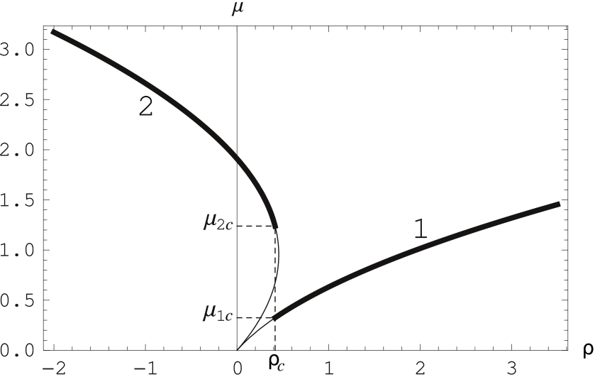
Figure 1: The dependence of $\mu=\frac{m}{\lambda}$ on $\rho=\frac{r}{\lambda^{2}}$. Quantities $r$ and $m$ are defined by Eqs. (2) and (2). The curves 1 and 2 represent the solutions $\mu_{1}(\rho)$ and $\mu_{2}(\rho)$ of Eq. (2). The bold curves show where these solutions correspond to the minimum of vacuum energy density (2). The $\rho_{c}$ is the point where this minimum is common for both solutions. The $\mu_{1c}$, $\mu_{2c}$ are limit values of $\mu_{1}(\rho)$, $\mu_{2}(\rho)$ as we approach to $\rho_{c}$ along bold parts of curves. We find from expressions (2), (2) $\rho_{c}\simeq 0.4157$, $\mu_{1c}\simeq 0.3248$ and $\mu_{2c}\simeq~{}1.2385$.

The curves 1 and 2 show the solutions $\mu_{1}(\rho)$ and $\mu_{2}(\rho)$ correspondingly. We consider these solutions at $\mu>0$. For any $\rho$ in the domain $0<\rho\leqslant\frac{9}{2\pi^{2}}$ (the largest value corresponds to the rightmost point of the curve 2) there are several distinct values of $\mu$ on the branches of curves with $\mu>0$. The direct evaluation of the quantity (2) shows that its minimum corresponds to points on the bold curves in Fig. 1. Indeed, we consider the r.h.s. of Eq. (2) for the curve 1 and upper part of the curve 2 at common value of $\rho$ and take the difference of these expressions. Using Eq. (2) and Eq. (2) we find the following finite result for this difference in the regularization removing limit:

$$\halign{\hbox to\displaywidth{$\hfil\displaystyle#\hfil$}\cr 0.0pt{\hfil$\displaystyle\hskip 10.00002pt minus 10.00002pt\frac{\lambda^{3}}{2}\left(\frac{1}{16}\left(2\mu_{1}^{4}+\mu_{2}^{4}\right)+\frac{1}{3\pi}\left(\mu_{1}^{3}-\mu_{2}^{3}\right)+\frac{\rho}{12}\left(\mu_{2}^{2}-\mu_{1}^{2}\right)\right).\hfil\hskip 10.00002pt minus 10.00002pt(17)\hfilneg\crcr}}$$

We estimate this expression numerically at different values of $\rho$ taking into account the explicit dependence of $\mu_{1}$, $\mu_{2}$ on $\rho$ according to Eq. (2). We find that this expression is positive at $\rho<\rho_{c}$ where $\rho_{c}$ is the value of $\rho$ for which the expression (2) is equal zero. For $\rho_{c}<\rho\leqslant\frac{9}{2\pi^{2}}$ this expression is negative. The $\mu_{1c}$ and $\mu_{2c}$ are the limit values of $\mu_{1}(\rho)$ and $\mu_{2}(\rho)$ in the limit transition $\rho\to\rho_{c}$ along bold parts of curves 1 and 2 respectively. Numerically we find $\rho_{c}\simeq 0.4157$, $\mu_{1c}\simeq 0.3248$ and $\mu_{2c}\simeq~{}1.2385$.

Analogous comparison for corresponding lower and upper points on the curve 2 gives the following expression:

$$\halign{\hbox to\displaywidth{$\hfil\displaystyle#\hfil$}\cr 0.0pt{\hfil$\displaystyle\hskip 10.00002pt minus 10.00002pt\frac{\lambda^{3}}{2}\left(\frac{1}{16}\left(\mu_{2}^{4}-\bar{\mu}_{2}^{4}\right)+\frac{1}{3\pi}\left(\bar{\mu}_{2}^{3}-\mu_{2}^{3}\right)+\frac{\rho}{12}\left(\mu_{2}^{2}-\bar{\mu}_{2}^{2}\right)\right),\hfil\hskip 10.00002pt minus 10.00002pt(18)\hfilneg\crcr}}$$

where $\bar{\mu}_{2}$ denotes lower point on the curve 2. Analogously we find numerically that this expression is positive at $\rho<\frac{9}{2\pi^{2}}$.

Thus we prove that the minimum of vacuum energy corresponds to the points on the bold curves. Therefore we have the following inequalities limiting the parameters $\lambda$, $m_{1}\equiv\lambda\mu_{1}$, $m_{2}\equiv\lambda\mu_{2}$ which one should use in calculations with our Hamiltonian:

$$\halign{\hbox to\displaywidth{$\hfil\displaystyle#\hfil$}\cr 0.0pt{\hfil$\displaystyle\hskip 10.00002pt minus 10.00002pt\frac{\lambda}{m_{1}}<\frac{1}{\mu_{1c}},\quad\text{i.e.}\quad\mu_{1}>\mu_{1c}\quad\text{for}\quad\varphi_{0}=0;\hfil\hskip 10.00002pt minus 10.00002pt\phantom{(19)}\hfilneg\cr 0.0pt{\hfil$\displaystyle\hfilneg\hskip 10.00002pt minus 10.00002pt\hfil\frac{\lambda}{m_{2}}<\frac{1}{\mu_{2c}},\quad\text{i.e.}\quad\mu_{2}>\mu_{2c}\quad\text{for}\quad\varphi_{0}^{2}=\frac{\,m_{2}^{2}}{8\lambda}.\hfil\hskip 10.00002pt minus 10.00002pt(19)\hfilneg\crcr}}}$$

Let us apply these results to the Hamiltonian (2). We define the $\tilde{\varphi}=\varphi-\varphi_{0}$ and rewrite the Hamiltonian in the normal ordered form w.r.t. those operators $a(k)$ and $a^{+}(k)$ which correspond to the found vacuum. Owing to Eq. (2) the resulting expression becomes dependent on the mass parameters $m_{1}$, $m_{2}$ only. These parameters correspond to solutions shown in Fig. 1. In the case $\varphi_{0}=0$ we get the following Hamiltonian (throwing out the constant term $\langle 0|{\cal H}|0\rangle$):

$$\halign{\hbox to\displaywidth{$\hfil\displaystyle#\hfil$}\cr 0.0pt{\hfil$\displaystyle\hskip 10.00002pt minus 10.00002ptH=\,:\int dy^{1}dy^{\bot}\left(\frac{(\Pi-\partial_{1}\tilde{\varphi})^{2}}{2\eta^{2}}+\frac{1}{2}\,(\partial_{\bot}\tilde{\varphi})^{2}+\frac{\,m_{1}^{2}}{2}\tilde{\varphi}^{2}+\lambda\tilde{\varphi}^{4}\right):,\hfil\hskip 10.00002pt minus 10.00002pt(20)\hfilneg\crcr}}$$

where the symbol ”: :” denotes the normal ordering. Analogously, in the case $\varphi_{0}^{2}=\frac{\,m_{2}^{2}}{8\lambda}$ we obtain

$$\halign{\hbox to\displaywidth{$\hfil\displaystyle#\hfil$}\cr 0.0pt{\hfil$\displaystyle\hskip 10.00002pt minus 10.00002ptH=\,:\int dy^{1}dy^{\bot}\left(\frac{(\Pi-\partial_{1}\tilde{\varphi})^{2}}{2\eta^{2}}+\frac{1}{2}\,(\partial_{\bot}\tilde{\varphi})^{2}+\frac{\,m_{2}^{2}}{2}\tilde{\varphi}^{2}+4\lambda\varphi_{0}\tilde{\varphi}^{3}+\lambda\tilde{\varphi}^{4}\right):.\hfil\hskip 10.00002pt minus 10.00002pt(21)\hfilneg\crcr}}$$

Here the terms linear in the fields $\tilde{\varphi},\Pi$ are discarded because they don’t contribute to the integral (2) due to the condition $|k_{1}|\geqslant\delta>0$ proposed earlier for the integration in formulae (2) and (2) (see the text before Eq. (2)).

To find the form of the LF Hamiltonian let us consider the eigenvalue problem:

$$\halign{\hbox to\displaywidth{$\hfil\displaystyle#\hfil$}\cr 0.0pt{\hfil$\displaystyle\hskip 10.00002pt minus 10.00002ptH|f\rangle=E|f\rangle,\hfil\hskip 10.00002pt minus 10.00002pt(22)\hfilneg\crcr}}$$

where the $H$ is the Hamiltonian (2) or (2). One can expand these Hamiltonians in powers of the parameter $\eta$. We separate the $\eta^{-2}$ term of these Hamiltonians and write them in the form

$$\halign{\hbox to\displaywidth{$\hfil\displaystyle#\hfil$}\cr 0.0pt{\hfil$\displaystyle\hskip 10.00002pt minus 10.00002ptH=\frac{H_{0}}{\eta^{2}}+H_{2},\hfil\hskip 10.00002pt minus 10.00002pt(23)\hfilneg\crcr}}$$

where

$$\halign{\hbox to\displaywidth{$\hfil\displaystyle#\hfil$}\cr 0.0pt{\hfil$\displaystyle\hskip 10.00002pt minus 10.00002ptH_{0}=2\int_{-\infty}^{0}dk_{1}\int dk_{\bot}|k_{1}|\,a^{+}(k)\,a(k).\hfil\hskip 10.00002pt minus 10.00002pt(24)\hfilneg\crcr}}$$

In the derivation of this expression we use the equality $\omega(k)=|k_{1}|+\frac{\eta^{2}(m^{2}+k_{\bot}^{2})}{|2k_{1}|}+~{}O(\eta^{4})$ following from the Eq. (2). Let us write the following asymptotic expansions:

$$\halign{\hbox to\displaywidth{$\hfil\displaystyle#\hfil$}\cr 0.0pt{\hfil$\displaystyle\hskip 10.00002pt minus 10.00002ptE(\eta)=\frac{E_{0}}{\eta^{2}}+E_{2}+\cdots,\qquad|f(\eta)\rangle=|f_{0}\rangle+\eta^{2}|f_{2}\rangle+\cdots\hfil\hskip 10.00002pt minus 10.00002pt(25)\hfilneg\crcr}}$$

In the lowest order approximation w.r.t. $\eta$ we obtain the equations:

$$\halign{\hbox to\displaywidth{$\hfil\displaystyle#\hfil$}\cr 0.0pt{\hfil$\displaystyle\hskip 10.00002pt minus 10.00002ptH_{0}|f_{0}\rangle=E_{0}|f_{0}\rangle\,,\qquad(H_{0}-E_{0})|f_{2}\rangle+(H_{2}-E_{2})|f_{0}\rangle=0.\hfil\hskip 10.00002pt minus 10.00002pt(26)\hfilneg\crcr}}$$

In the limit $\eta\to 0$ we have $x^{1}\to x^{-},\,\,|f\rangle\to|f_{0}\rangle$, i.e. the states $|f_{0}\rangle$ form the state space on the LF. To get finite eigenvalues for the LF Hamiltonian we demand $E_{0}=0$. Then from the Eq. (2) and the first of Eqs. (2) we obtain

$$\halign{\hbox to\displaywidth{$\hfil\displaystyle#\hfil$}\cr 0.0pt{\hfil$\displaystyle\hskip 10.00002pt minus 10.00002pta(k)|f_{0}\rangle=0\quad\text{at}\quad k_{1}<0.\hfil\hskip 10.00002pt minus 10.00002pt(27)\hfilneg\crcr}}$$

Therefore in the limit $\eta\to 0$ the LF state space is the subspace of our Fock space in which only the quanta with $k_{-}>0$ are present. Now let us take the projection of the second of the Eqs. (2) on the subspace of states $|f_{0}\rangle$ and denote by ${\cal P}$ the projector on this subspace. Then we get the equation which can be interpreted as the eigenvalue equation for the LF Hamiltonian. So now we have

$$\halign{\hbox to\displaywidth{$\hfil\displaystyle#\hfil$}\cr 0.0pt{\hfil$\displaystyle\hskip 10.00002pt minus 10.00002ptH_{LF}={\cal P}H_{2}{\cal P}.\hfil\hskip 10.00002pt minus 10.00002pt(28)\hfilneg\crcr}}$$

Using the expressions (2) and (2) and the equality (2) we obtain the following results:

$$\halign{\hbox to\displaywidth{$\hfil\displaystyle#\hfil$}\cr 0.0pt{\hfil$\displaystyle\hskip 10.00002pt minus 10.00002ptH_{LF}=\,:\int dx^{-}dx^{\bot}\left(\frac{1}{2}\,(\partial_{\bot}\Phi)^{2}+\frac{\,m_{1}^{2}}{2}\Phi^{2}+\lambda\Phi^{4}\right):\hfil\hskip 10.00002pt minus 10.00002pt(29)\hfilneg\crcr}}$$

for the case $\varphi_{0}=0$ and

$$\halign{\hbox to\displaywidth{$\hfil\displaystyle#\hfil$}\cr 0.0pt{\hfil$\displaystyle\hskip 10.00002pt minus 10.00002ptH_{LF}=\,:\int dx^{-}dx^{\bot}\left(\frac{1}{2}\,(\partial_{\bot}\Phi)^{2}+\frac{\,m_{2}^{2}}{2}\Phi^{2}+4\lambda\varphi_{0}\Phi^{3}+\lambda\Phi^{4}\right):\hfil\hskip 10.00002pt minus 10.00002pt(30)\hfilneg\crcr}}$$

for the case $\varphi_{0}^{2}=\frac{\,m_{2}^{2}}{8\lambda}$. Here we denote by $\Phi(x)$ the field on the LF,

$$\halign{\hbox to\displaywidth{$\hfil\displaystyle#\hfil$}\cr 0.0pt{\hfil$\displaystyle\hskip 10.00002pt minus 10.00002pt\Phi(x)=\frac{1}{2\pi}\int_{\delta}^{\infty}\frac{dk_{-}}{\sqrt{2k_{-}}}\int dk_{\bot}\left(a(k_{-},k_{\bot})\,e^{-ik\cdot x}+a^{+}(k_{-},k_{\bot})\,e^{ik\cdot x}\right),\hfil\hskip 10.00002pt minus 10.00002pt(31)\hfilneg\crcr}}$$

where $k\cdot x=k_{-}x^{-}+k_{\bot}x^{\bot}$. The operators $a^{+}(k_{-},k_{\bot})$ and $a(k_{-},k_{\bot})$ play the role of creation and annihilation operators in the LF Fock space. They satisfy canonical commutation relations on the LF. Note that the integration range in Eq. (2) is limited from below by a small parameter $\delta$ which we implicitly use in the Eqs. (2), (2) (see the text before Eq. (2)).

3 Investigation of perturbation theory

In the previous section we have obtained in Gaussian approximation the LF Hamiltonians (2), (2). The theories described by these LF Hamiltonians contain UV divergences. To study these divergences and carry out the renormalization let us compare the perturbation theories, generated by these LF Hamiltonians, with the corresponding renormalized covariant perturbation theories in Lorentz coordinates (in all orders). With this aim we consider the covariant perturbation theory for the Lagrangian in the following general form (in Lorentz coordinates):

$$\halign{\hbox to\displaywidth{$\hfil\displaystyle#\hfil$}\cr 0.0pt{\hfil$\displaystyle\hskip 10.00002pt minus 10.00002pt{\cal L}=\frac{1}{2}\partial_{\mu}\varphi\partial^{\mu}\varphi-\frac{m^{2}}{2}\varphi^{2}-\gamma\varphi-g\varphi^{3}-\lambda\varphi^{4}.\hfil\hskip 10.00002pt minus 10.00002pt(32)\hfilneg\crcr}}$$

Standard analysis shows that this theory is superrenormalizable, i.e. it has only finite number of divergent diagrams which must be renormalized. These diagrams are shown in Fig. 2.

Figure 2: The divergent diagrams.

The sum of all connected diagrams with one external line (”tadpole” diagrams) gives the one-point Green function. It is a constant in the coordinate space and is equal to the vacuum average of the field $\varphi$. So one can make this constant to be equal to zero by the shift of the field: $\varphi\to\varphi-\varphi_{0}$, where $\varphi_{0}$ is the constant. In this way we obtain the theory without tadpole diagrams (and subdiagrams). The linear in the field term of the Lagrangian (3) generates only the tadpole subdiagrams. Therefore if we consider the perturbation theory without tadpole subdiagrams, we can ignore this term in the Lagrangian. The parameter $\lambda$ in the Lagrangian (3) does not change after the shift in the field, while the parameters $m^{2}$ and $g$ do change.

The diagrams with two external lines joined to one vertex (we denote them by ”tadpole-2” diagrams) do not depend on external momenta. All such connected diagrams are one-particle-irreducible ones (in the absence of the tadpole subdiagrams), and their contribution is equivalent to the addition of the counterterm, quadratic in the field, to the Lagrangian. In this way one can formulate the perturbation theory in Lorentz coordinates without tadpole and tadpole-2 diagrams (and corresponding subdiagrams).

Then we have only one logarithmically divergent diagram, the divergent part of which must be compensated by the counterterm quadratic in the field. This diagram is shown in Fig. 2 (f), and in the following we denote it by $I(p)$. Further we choose the PV method for the regularization of the obtained perturbation theory. This choice requires the introduction of the auxiliary large mass $M$ ghost field $\varphi_{g}(x)$ into the Lagrangian.

Thus we can generate the considered perturbation theory in Lorentz coordinates by the following regularized Lagrangian if we throw away all tadpole and tadpole-2 diagrams:

$$\halign{\hbox to\displaywidth{$\hfil\displaystyle#\hfil$}\cr 0.0pt{\hfil$\displaystyle\hskip 10.00002pt minus 10.00002pt{\cal L}=\frac{1}{2}\left(\partial_{\mu}\varphi\partial^{\mu}\varphi-\tilde{m}^{2}\varphi^{2}\right)-\frac{1}{2}\left(\partial_{\mu}\varphi_{g}\partial^{\mu}\varphi_{g}-M^{2}\varphi_{g}^{2}\right)-\frac{3\lambda^{2}}{\pi^{2}}\left(\ln\frac{M}{\tilde{m}}\right)\left(\varphi+\varphi_{g}\right)^{2}-\hfill\cr 0.0pt{\hfil$\displaystyle\hfill-\tilde{g}\left(\varphi+\varphi_{g}\right)^{3}-\lambda\left(\varphi+\varphi_{g}\right)^{4}.\hfil\hskip 10.00002pt minus 10.00002pt(33)\hfilneg\crcr}}}$$

Here the mass $M$ is the regularization parameter, and the quadratic in the field $(\varphi+\varphi_{g})$ counterterm is added to compensate the divergent part of the diagram $I(p)$ at $M\to\infty$. This divergent part is calculated in Appendix A.

Now let us write the canonical Hamiltonian on the LF, corresponding to this Lagrangian, and take this Hamiltonian in the normally ordered form (in accordance with the absence of the tadpole and tadpole-2 diagrams in the previously considered perturbation theory in Lorentz coordinates):

$$\halign{\hbox to\displaywidth{$\hfil\displaystyle#\hfil$}\cr 0.0pt{\hfil$\displaystyle\hskip 10.00002pt minus 10.00002ptH_{LF}=\,:\int dx^{-}dx^{\bot}\Biggl{(}\frac{1}{2}\left(\partial_{\bot}\Phi\right)^{2}-\frac{1}{2}\left(\partial_{\bot}\Phi_{g}\right)^{2}+\frac{\,\tilde{m}^{2}}{2}\,\Phi^{2}-\frac{\,M^{2}}{2}\,\Phi_{g}^{2}+\hfill\cr 0.0pt{\hfil$\displaystyle\hfill+\frac{3\lambda^{2}}{\pi^{2}}\left(\ln\frac{M}{\tilde{m}}\right)\left(\Phi+\Phi_{g}\right)^{2}+\tilde{g}\left(\Phi+\Phi_{g}\right)^{3}+\lambda\left(\Phi+\Phi_{g}\right)^{4}\Biggr{)}:.\hfil\hskip 10.00002pt minus 10.00002pt(34)\hfilneg\crcr}}}$$

Here we introduce, like in the Eq. (2), the regularization parameter $\delta$ for the Fourier decomposition of fields $\varphi$ and $\varphi_{g}$ in terms of creation and annihilation operators on the LF, and again denote these regularized fields by $\Phi$ and $\Phi_{g}$. The canonical commutation relations for the ghost creation and annihilation operators have the opposite sign w.r.t. conventional ones.

Starting from this Hamiltonian we can generate the same set of diagrams as in covariant perturbation theory in Lorentz coordinates. Indeed, it was proven in paper [45] that each term in covariant perturbation theory (i.e. Feynman diagram) can be written as the sum of terms in the $x^{+}$-ordered (”old-fashioned”) perturbation theory series. But the difference is contained in the way of calculation of diagrams: for LF perturbation theory the integration must be carried out firstly over the momenta $k_{+}$ and the condition $|k_{-}|\geqslant\delta$ must be introduced as the regularization of fields in Eq. (3).

Let us remark that this way of calculation gives all tadpole and tadpole-2 diagrams equal to zero. Indeed, the tadpole diagrams are absent because the momentum of the external line of these diagrams is equal to zero but the regularization of fields on the LF ($|k_{-}|\geqslant\delta$) doesn’t allow such external momentum. Tadpole-2 diagrams are equal zero because in such a diagram there is always a closed loop that has the same sign of the loop momentum $q_{-}$ in all its propagators. As the result the residue integral w.r.t. corresponding loop momentum $q_{+}$ is equal to zero, because all poles related to these propagators lie on the same side of the real axis of $q_{+}$. Two divergent tadpole-2 diagrams shown in Fig. 2 (d), (e) are absent due to normal ordering of the Hamiltonian (3). So the set of nonzero diagrams turns out to be the same in perturbation theory in Lorentz coordinates and that generated by the Hamiltonian on the LF.

However it is known that the corresponding diagrams calculated in each of these perturbation theories can differ [18, 19, 4]. One can use the method of the papers [19, 4] to compare such diagrams in all orders of perturbation theory. The idea of this method is the following. The diagrams generated by the LF Hamiltonian are regularized with the $|k_{-}|\geqslant\delta$ cutoff. Therefore the difference between the result of calculation of such a diagram and the result of calculation of the corresponding covariant diagram in Lorentz coordinates reduces to the integrals over the region $|k_{-}|\leqslant\delta$ of each propagator. If one makes for each loop momentum $q$ (which can be always identified with a some propagator momentum) the change $q_{-}\to q_{-}\delta$, $q_{+}\to q_{+}/\delta$ an essential dependence on $\delta$ in the integration region disappears, and one can investigate the behavior of the integrand at $\delta\to 0$ for an arbitrarily complicated diagram using only general properties of the theory (Lorentz invariance, the spin of the field, the structure of the propagator, etc.). With this method it is possible to prove for our model that the results of calculation of any diagram in the LF perturbation theory and in the covariant perturbation theory in Lorentz coordinates coincide in the limit $\delta\to 0$ (taking into account the absence of tadpole and tadpole-2 diagrams). In Appendix B we illustrate how this method works with the example of one-loop diagram.

Thus the theory with the LF Hamiltonian (3) turns out to be equivalent in all orders of perturbation theory to the conventional renormalized covariant perturbation theory in Lorentz coordinates in the limit $\delta\to 0$ (and then $M\to\infty$).

Therefore the Eq. (3) gives the perturbatively renormalized LF Hamiltonian. We notice that the LF Hamiltonian (3) can be considered, at definite choice of its parameters, as one of the LF Hamiltonians (2), (2), correspondingly regularized and renormalized. The coupling constant $\tilde{g}$ can be identified with $4\lambda\varphi_{0}$ ($\varphi_{0}=0$ or $\varphi_{0}^{2}=\frac{m_{2}^{2}}{8\lambda}$), while $\tilde{m}$ can be identified with $m_{1}$ or $m_{2}$ for the LF Hamiltonians (2) and (2) respectively. Thus we obtain the renormalized LF Hamiltonians for the cases without and with the spontaneous symmetry breaking. The parameters $m_{1}$, $m_{2}$ and $\lambda$ satisfy the inequalities (2) in the Gaussian approximation. Nevertheless one can assume that these inequalities are approximately valid for the renormalized LF Hamiltonians in the PV regularization.

4 Conclusion

In the present paper we have constructed the renormalized LF Hamiltonian for the $\lambda\varphi^{4}$ model in (2+1)-dimensional space-time. We have found the explicit expression for the counterterm, necessary for the renormalization, using the PV regularization. To do this we compare the diagrams of the covariant perturbation theory in Lorentz coordinates with the analogous diagrams of the perturbation theory generated by the LF Hamiltonian which has also the cutoff in the momentum $p_{-}$ ($|p_{-}|\geqslant\delta>0$). We show that both perturbation theories can be described by the same set of diagrams, with the values of the compared diagrams coinciding in the limit $\delta\to 0$. Then we renormalize the LF Hamiltonian by the counterterm found in the calculation of the divergent part of the corresponding diagram in the covariant perturbation theory in Lorentz coordinates.

Furthermore we have taken into account the possibility of the spontaneous symmetry breaking in this model and obtained the LF Hamiltonians corresponding to two different vacua. We arrive at these LF Hamiltonians by considering the limit transition from the theories quantized on the spacelike planes approaching the LF. It is possible to describe the vacuum on these planes using the Gaussian approximation. The Hamiltonians obtained with this approximation still require UV renormalization. And the above-mentioned comparison of perturbative theories, generated by these LF Hamiltonians, and the covariant perturbation theory in Lorentz coordinates allows to renormalize both of these Hamiltonians in the PV regularization.

Having such LF Hamiltonians one can start nonperturbative calculation of the mass spectrum solving the eigenvalue problem:

$$\halign{\hbox to\displaywidth{$\hfil\displaystyle#\hfil$}\cr 0.0pt{\hfil$\displaystyle\hskip 10.00002pt minus 10.00002pt(2P_{-}H_{LF}-P_{\bot}^{2})|p_{-},p_{\bot}\rangle=m^{2}|p_{-},p_{\bot}\rangle.\hfil\hskip 10.00002pt minus 10.00002pt(35)\hfilneg\crcr}}$$

This calculation could help to study the peculiarities of the PV regularization related to the presence of ghost fields and states with the indefinite metric. That is important for the application of this method to QCD.

To solve the eigenvalue problem (4) nonperturbatively one can apply numerical approach using the discretization of the momenta: $p_{-}=\frac{\pi n}{L},\,n=0,1,2,\ldots$; $p_{\bot}=\frac{\pi n_{\bot}}{L_{\bot}}$, ${n_{\bot}=0,\pm 1,\pm 2,\ldots}$ This discretization is achieved by introducing the limits ${|x^{-}|\leqslant L}$, $|x^{\bot}|\leqslant L_{\bot}$ and corresponding periodic boundary conditions for fields (see e.g. [26, 28, 29]). Also it is useful to introduce the lattice in $x^{\bot}$ to limit the $n_{\bot}$. This calculation must be carried out at finite but increasing values of the parameters $M,L,L_{\bot}$ and the cutoff in $n_{\bot}$. As it was shown in the papers [19, 4] the regularization $|p_{-}|\geqslant\delta>0$ must be removed before the removing of PV regularization. In the DLCQ (with zero modes ($p_{-}=0$) being thrown out) one can put $\delta=\frac{\pi}{L}$. So we must at first take $L\to\infty$. For finite total momentum $p_{-}=\frac{\pi n}{L}$ this limit is equivalent to $n\to\infty$. The successful calculation of few lowest values of mass in QED(1+1) [23] for all values of the coupling (including very large ones) shows the possibility to make the extrapolation to $n\to\infty$ using the results obtained at finite values of $n$. One can assume that such extrapolation may be done at every fixed values of $M$, $L_{\bot}$ and lattice parameter. It must be noticed that in such calculations zero modes of fields ($p_{-}=0$), playing important role for correct description of possible vacuum effects [40], are excluded because in the considered scalar field theory the effect of spontaneous symmetry breaking can be approximately taken into account. In gauge theories like QCD these zero modes can be included into LF canonical formalism [46] where they are to be defined via solution of complicated second class constraints that remains the difficult problem. Correct description of vacuum effects with the LF Hamiltonian can be given for QED(1+1) [21, 23] and the role of zero modes can be seen there.

The generalization of these methods to gauge theories requires the construction of renormalized LF Hamiltonians for these theories. A possible way to construct such Hamiltonians in PV regularization was proposed for light-cone gauge QCD(3+1) in [20, 4] and applied for calculation of anomalous magnetic moment in QED(3+1) [30].

The AdS/QCD correspondence and its relation to QCD bound state problem [42, 43, 47, 48] suggests the description of bound state wave functions in terms of some special functions different from usual plane wave ones. This implies that the basis functions used in the decomposition of fields in terms of light-front creation and annihilation operators can be chosen in accordance with those special functions in a hope to make the solution of Eq. (4) more effective. This approach was applied in papers [49, 50, 51].

Despite of difficulties these methods meet one hopes that the LF quantization could give frame-invariant and unified scheme for the description of hadron physics at high energies and, nonperturbatively, at lower energies [3].

Acknowledgments. We thank M.V. Kompaniets and V.A. Franke for useful discussions. The authors M.Yu.M., E.V.P. and R.A.Z. acknowledge Saint-Petersburg State University for a research grant 11.38.189.2014.

Appendix A. The calculation of the diagram $I(p)$

For the renormalization of our model in the conventional Feynman covariant perturbation theory it is necessary to consider only one logarithmically divergent diagram (Fig. 2 (f)). This diagram in the PV regularization has the following form:

$$\halign{\hbox to\displaywidth{$\hfil\displaystyle#\hfil$}\cr 0.0pt{\hfil$\displaystyle\hskip 10.00002pt minus 10.00002ptI(\vec{p})=\frac{96i\lambda^{2}}{(2\pi)^{6}}\int d^{3}\vec{k}_{1}\,d^{3}\vec{k}_{2}\,d^{3}\vec{k}_{3}\,\delta\left(\sum_{j=1}^{3}\vec{k}_{j}-\vec{p}\right)\prod_{j=1}^{3}\left(\frac{1}{\vec{k}_{j}^{2}+m^{2}}-\frac{1}{\vec{k}_{j}^{2}+M^{2}}\right),\hfil\hskip 10.00002pt minus 10.00002pt(36)\hfilneg\crcr}}$$

where the integration is over the Euclidean momenta, the parameter $m$ is the mass parameter, the $M$ is PV regularization parameter, the factor $96=(4!)^{2}/6$ includes the symmetry coefficient 1/6 of this diagram (the factor $(4!)^{2}$ is related to the definition of the coupling $\lambda$ in the Lagrangian (3)). To find the counterterm we need to calculate only the divergent (at $M\to\infty$) part of the $I(\vec{p})$. This divergent part can be evaluated as the divergent part of the $I(\vec{p})|_{\vec{p}=0}$ which can be rewritten in the following form:

$$\halign{\hbox to\displaywidth{$\hfil\displaystyle#\hfil$}\cr 0.0pt{\hfil$\displaystyle\hskip 10.00002pt minus 10.00002ptI(0)=\frac{96i\lambda^{2}}{(2\pi)^{9}}\int d^{3}\vec{x}\,\,e^{i\vec{x}(\vec{k}_{1}+\vec{k}_{2}+\vec{k}_{3})}\prod_{j=1}^{3}\int d^{3}\vec{k}_{j}\left(\frac{1}{\vec{k}_{j}^{2}+m^{2}}-\frac{1}{\vec{k}_{j}^{2}+M^{2}}\right)=\hfill\cr 0.0pt{\hfil$\displaystyle\hfill=\frac{3i\lambda^{2}}{16\pi^{9}}\int d^{3}\vec{x}\left(\int d^{3}\vec{k}\,\,e^{i\,\vec{k}\vec{x}}\left(\frac{1}{\vec{k}^{2}+m^{2}}-\frac{1}{\vec{k}^{2}+M^{2}}\right)\right)^{3}.\hfil\hskip 10.00002pt minus 10.00002pt(37)\hfilneg\crcr}}}$$

We can use the well-known result:

$$\halign{\hbox to\displaywidth{$\hfil\displaystyle#\hfil$}\cr 0.0pt{\hfil$\displaystyle\hskip 10.00002pt minus 10.00002pt\int d^{3}\vec{k}\frac{e^{i\vec{k}\vec{x}}}{\vec{k}^{2}+m^{2}}=\frac{2\pi^{2}}{r}e^{-rm},\quad r=\sqrt{\vec{x}^{2}}.\hfil\hskip 10.00002pt minus 10.00002pt(38)\hfilneg\crcr}}$$

To obtain this result it is sufficient to put $\vec{x}=\{r,0,0\}$ and evaluate residue integral:

$$\halign{\hbox to\displaywidth{$\hfil\displaystyle#\hfil$}\cr 0.0pt{\hfil$\displaystyle\hskip 10.00002pt minus 10.00002pt\int d^{3}\vec{k}\frac{e^{ik_{1}r}}{k_{1}^{2}+k_{2}^{2}+k_{3}^{2}+m^{2}}=2\pi i\int dk_{2}\,dk_{3}\frac{e^{-r\sqrt{k_{2}^{2}+k_{3}^{2}+m^{2}}}}{2i\sqrt{k_{2}^{2}+k_{3}^{2}+m^{2}}}=\frac{2\pi^{2}}{r}e^{-rm}.\hfil\hskip 10.00002pt minus 10.00002pt(39)\hfilneg\crcr}}$$

Further we substitute this result into Eq. (Appendix A. The calculation of the diagram $I(p)$):

$$\halign{\hbox to\displaywidth{$\hfil\displaystyle#\hfil$}\cr 0.0pt{\hfil$\displaystyle\hskip 10.00002pt minus 10.00002ptI(0)=\frac{6i\lambda^{2}}{\pi^{2}}\int_{0}^{\infty}\frac{dr}{r}\left(e^{-rm}-e^{-rM}\right)^{3}=\frac{6i\lambda^{2}}{\pi^{2}}\biggl{(}\int_{0}^{1}\frac{dr}{r}\left(e^{-r\frac{m}{M}}-e^{-r}\right)^{3}+\hfill\cr 0.0pt{\hfil$\displaystyle\hfill+\int_{1}^{\infty}\frac{dr}{r}e^{-3r\frac{m}{M}}+\int_{1}^{\infty}\frac{dr}{r}\left(-3e^{-2r\frac{m}{M}}e^{-r}+3e^{-r\frac{m}{M}}e^{-2r}-e^{-3r}\right)\biggr{)}.\hfil\hskip 10.00002pt minus 10.00002pt(40)\hfilneg\crcr}}}$$

The first and third integrals in this expression are finite constants at $M\to\infty$, and therefore, the $I(0)$ can be rewritten as follows:

$$\halign{\hbox to\displaywidth{$\hfil\displaystyle#\hfil$}\cr 0.0pt{\hfil$\displaystyle\hskip 10.00002pt minus 10.00002ptI(0)=\frac{6i\lambda^{2}}{\pi^{2}}\int_{1}^{\infty}\frac{dr}{r}e^{-3r\frac{m}{M}}+O(1)=\frac{6i\lambda^{2}}{\pi^{2}}\int_{\frac{m}{M}}^{\infty}\frac{dr}{r}e^{-3r}+O(1)=\hfill\cr 0.0pt{\hfil$\displaystyle\hfill=\frac{6i\lambda^{2}}{\pi^{2}}\left(\int_{1}^{\infty}\frac{dr}{r}e^{-3r}+\int_{\frac{m}{M}}^{1}\frac{dr}{r}\left(e^{-3r}-1\right)+\int_{\frac{m}{M}}^{1}\frac{dr}{r}\right)+O(1).\hfil\hskip 10.00002pt minus 10.00002pt(41)\hfilneg\crcr}}}$$

The first two integrals in this expression are finite constants at $M\to\infty$, thus we obtain for $I(0)$ the following result:

$$\halign{\hbox to\displaywidth{$\hfil\displaystyle#\hfil$}\cr 0.0pt{\hfil$\displaystyle\hskip 10.00002pt minus 10.00002ptI(0)=\frac{6i\lambda^{2}}{\pi^{2}}\ln{\frac{M}{m}}+O(1).\hfil\hskip 10.00002pt minus 10.00002pt(42)\hfilneg\crcr}}$$

Using this result one can find the corresponding counterterm in the standard way [44]. This counterterm is present in the Eqs. (3) and (3).

Appendix B. The example of comparison of diagram calculations

Let us demonstrate how the method of comparison of calculations in LF and usual covariant perturbation theory [4, 19] works using as an example the 1-loop diagram with two external lines. Let us write the corresponding integrand in the following form:

$$\halign{\hbox to\displaywidth{$\hfil\displaystyle#\hfil$}\cr 0.0pt{\hfil$\displaystyle\hskip 10.00002pt minus 10.00002pt\frac{1}{\left(q^{2}-m^{2}+i0\right)\left((q+p)^{2}-m^{2}+i0\right)}=\hfill\cr 0.0pt{\hfil$\displaystyle\hfill=\frac{1}{\left(2q_{+}q_{-}-q_{\bot}^{2}-m^{2}+i0\right)\left(2(q_{+}+p_{+})(q_{-}+p_{-})-(q_{\bot}+p_{\bot})^{2}-m^{2}+i0\right)},\hfil\hskip 10.00002pt minus 10.00002pt(43)\hfilneg\crcr}}}$$

where $p$ and $q$ are external and loop momenta respectively.

In the calculation of diagrams in usual covariant perturbation theory the integration is carried out over all momenta $q_{\mu}$ while in the LF calculation the integration is only over the domain $\{|q_{-}|\geqslant\delta\}\cap\{|q_{-}+p_{-}|\geqslant\delta\}$ due to the regularization of fields in Eq. (3). So the difference between the LF and the conventional covariant calculations of the diagram is given by the integral over the domain $\{|q_{-}|<\delta\}\cup\{|q_{-}+p_{-}|<\delta\}$. This domain consists of two parts and the contribution of each of them should be considered separately. However the contribution of the second part becomes similar to one of the first part after the change $q\to\tilde{q}=q+p$. So we consider the integration only over the first part of the integration domain:

$$\halign{\hbox to\displaywidth{$\hfil\displaystyle#\hfil$}\cr 0.0pt{\hfil$\displaystyle\hskip 10.00002pt minus 10.00002pt\int dq_{\bot}\int dq_{+}\int_{-\delta}^{\delta}dq_{-}\frac{1}{\left(2q_{+}q_{-}-q_{\bot}^{2}-m^{2}+i0\right)}\times\hfill\cr 0.0pt{\hfil$\displaystyle\hfill\times\frac{1}{\left(2(q_{+}+p_{+})(q_{-}+p_{-})-(q_{\bot}+p_{\bot})^{2}-m^{2}+i0\right)}.\hfil\hskip 10.00002pt minus 10.00002pt(44)\hfilneg\crcr}}}$$

After the change $q_{-}\to q_{-}\delta$, $q_{+}\to q_{+}/\delta$ this integral takes the form:

$$\halign{\hbox to\displaywidth{$\hfil\displaystyle#\hfil$}\cr 0.0pt{\hfil$\displaystyle\hskip 10.00002pt minus 10.00002pt\int dq_{\bot}\int dq_{+}\int_{-1}^{1}dq_{-}\frac{1}{\left(2q_{+}q_{-}-q_{\bot}^{2}-m^{2}+i0\right)}\times\hfill\cr 0.0pt{\hfil$\displaystyle\hfill\times\frac{\delta}{\left(2(q_{+}+p_{+}\delta)(p_{-}+q_{-}\delta)-(q_{\bot}+p_{\bot})^{2}\delta-m^{2}\delta+i0\right)}.\hfil\hskip 10.00002pt minus 10.00002pt(45)\hfilneg\crcr}}}$$

The integration domain is now independent on $\delta$ while the expression for the integrand can be easily analyzed in the $\delta\to 0$ limit. We see that in this limit the integral (Appendix B. The example of comparison of diagram calculations) is equal to zero.

If we add in the expression (Appendix B. The example of comparison of diagram calculations) the factor $q_{+}$ in the numerator (as e.g. in fermion self-energy diagram in Yukawa model, see [4, 19]) we get after the change $q_{+}\to q_{+}/\delta$ the additional factor $1/\delta$. So we obtain nonzero result for the difference between LF and conventional covariant calculations of such diagram. We see that the dependence on the external momenta factorizes in this result for the considered difference. Such factorization usually has place also in higher orders of perturbation theory [4, 19]. This gives a possibility to determine the form of necessary counterterms which must be added to the canonical LF Hamiltonian to remove the above-mentioned difference.

References

- [1] Dirac, P.A.M.: Forms of relativistic dynamics. Rev. Mod. Phys. 21(3), 392-398 (1949)
- [2] Brodsky, S.J., Pauli, H.-C., Pinsky, S.S.: Quantum Chromodynamics and other field theories on the light cone. Phys. Rep. 301(4-6), 299-486 (1998), arXiv:hep-ph/9705477 and references therein
- [3] Bakker, B.L.G., Bassetto, A., Brodsky, S.J., Broniowski, W., Dalley, S., Frederico, T., Glazek, S.D., Hiller, J.R., Ji, C.-R., Karmanov, V., Kulshreshtha, D., Mathiot, J.-F. at al. Light-Front Quantum Chromodynamics: A framework for the analysis of hadron physics, arXiv:1309.6333 [hep-ph]
- [4] Franke, V.A., Novozhilov, Yu.V., Paston, S.A., Prokhvatilov, E.V.: Quantization of Field Theory on the Light Front. In: Kovras, O. (ed.) Focus on quantum field theory, pp. 23-81. Nova science publishers, New York (2005), arXiv:hep-th/0404031
- [5] Annenkova A.M., Prokhvatilov, E.V., Franke, V.A.: The solution of Schrödinger equation on the light front for Sine-Gordon model. Vestn. Leningrad. Univ. (Ser. 4. Fiz. Khim.) 18, 80-83 (1985)
- [6] Brodsky, S.J., Pauli, H.-C. Discretized light-cone quantization: Solution to a field theory in one space and one time dimension. Phys. Rev. D 32(8), 2001-2013 (1985)
- [7] Eller, T., Pauli, H.-C., Brodsky, S.J. Discretized light-cone quantization: The massless and the massive Schwinger model. Phys. Rev. D 35(4), 1493-1507 (1987)
- [8] Hornbostel, K., Brodsky, S.J., Pauli, H.-C.: Light-cone-quantized QCD in 1+1 dimensions. Phys. Rev. D 41(12), 3814-3821 (1990)
- [9] Brodsky, S.J., Roskies, R, Suaya, R: Quantum Electrodynamics and Renormalization Theory in the Infinite-Momentum Frame. Phys. Rev. D 8(12), 4574-4594 (1973)
- [10] Srivastava, P.P., Brodsky, S.J. Light-front-quantized QCD in the light-cone gauge: The doubly transverse gauge propagator. Phys. Rev. D 64(4), 045006 (2001), arXiv:hep-ph/0011372v2
- [11] Glazek, S.D., Wilson, K.G.: Renormalization of Hamiltonians. Phys. Rev. D 48(8), 4214-4218 (1993)
- [12] Glazek, S.D., Wilson, K.G.: Perturbative renormalization group for Hamiltonians. Phys. Rev. D 49(12), 5863-5872 (1994)
- [13] Wilson, K.G., Walhout, T.S., Harindranath, A., Zhang, W.-M., Perry, R.J., Glazek, S.D.: Nonperturbative QCD: A Weak-Coupling Treatment on the Light Front. Phys. Rev. D 49(12), 6720-6766 (1994), arXiv:hep-th/9401153
- [14] Glazek, S.D.: Renormalization of Hamiltonians in the Light-Front Fock Space, arXiv:hep-th/9706212
- [15] Glazek, S.D.: Renormalization group and bound states. Acta Phys.Polon. B 39, 3395-3421 (2008), arXiv:0810.5258 [hep-th]
- [16] Glazek, S.D.: Dynamics of Effective Gluons. Phys. Rev. D 63(11), 116006 (2001), arXiv:hep-th/0012012
- [17] Glazek, S.D., Wieckowski, M.: Large-momentum convergence of Hamiltonian bound-state dynamics of effective fermions in quantum field theory. Phys. Rev. D 66(1), 016001 (2002), arXiv:hep-th/0204171
- [18] Burkardt, M., Langnau, A.: Hamiltonian formulation of (2+1)-dimensional QED on the light cone. Phys. Rev. D 44(4), 1187-1197 (1991). Rotational invariance in light-cone quantization. Phys. Rev. D. 44(12), 3857-3867 (1991)
- [19] Franke, V.A., Paston, S.A.: Comparison of quantum field perturbation theory for the light front with the theory in Lorentz coordinates. Theor. Math. Phys. 112(3), 1117-1130 (1997), arXiv:hep-th/9901110
- [20] Paston, S.A., Prokhvatilov, E.V., Franke, V.A.: Constructing the light-front QCD Hamiltonian. Theor. Math. Phys. 120(3), 1164-1181 (1999), arXiv:hep-th/0002062
- [21] Paston, S.A., Prokhvatilov, E.V., Franke, V.A.: The Light-Front Hamiltonian Formalism for Two-Dimensional Quantum Electrodynamics Equivalent to the Lorentz-Covariant Approach. Theor. Math. Phys. 131(1), 516-526 (2002), arXiv:hep-th/0302016
- [22] Ilgenfritz, E.M., Franke, V.A., Paston, S.A., Pirner, H.J., Prokhvatilov, E.V.: Quantum fields on the light front, formulation in coordinates close to the light front, lattice approximation. Theor. Math. Phys. 148(1), 948-959 (2006), arXiv:hep-th/0610020
- [23] Paston, S.A., Prokhvatilov, E.V., Franke, V.A.: Calculation of the Mass Spectrum of QED-2 in Light-Front Coordinates. Phys. Atom. Nucl. 68, 267-278 (2005), arXiv:hep-th/0501186
- [24] Sriganesh, P., Hamer, C.J., Bursill, R.J.: New finite-lattice study of the massive Schwinger model. Phys. Rev. D 62(3), 034508 (2000), arXiv:hep-lat/9911021
- [25] Pauli, W., Villars, F.: On the Invariant Regularization in Relativistic Quantum Theory. Rev. Mod. Phys. 21(3), 434-444 (1949)
- [26] Brodsky, S.J., Hiller, J.R., McCartor, G.: Application of Pauli-Villars regularization and discretized light-cone quantization to a single-fermion truncation of Yukawa theory. Phys. Rev. D 64(11), 114023 (2001), arXiv:hep-ph/0107038
- [27] Brodsky, S.J., Hiller, J.R., McCartor, G.: Exact Solutions to Pauli-Villars-Regulated Field Theories. Ann. Phys. 296(2), 406-424 (2002), arXiv:hep-th/0107246
- [28] Brodsky, S.J., Hiller, J.R., McCartor, G.: Application of Pauli-Villars regularization and Discretized Light-Cone Quantization to a (3+1)-Dimensional Model. Phys. Rev. D 60(5), 054506 (1999), arXiv:hep-ph/9903388
- [29] Brodsky, S.J., Hiller, J.R., McCartor, G.: Pauli-Villars as a Nonperturbative Ultraviolet Regulator in Discretized Light-Cone Quantization. Phys. Rev. D 58(2), 025005 (1998), arXiv:hep-th/9802120
- [30] Brodsky, S.J., Franke, V.A., Hiller, J.R., McCartor, G., Paston, S.A., Prokhvatilov, E.V.: A nonperturbative calculation of the electron’s magnetic moment. Nucl. Phys. B 703, 333-362 (2004), arXiv:hep-ph/0406325
- [31] Chabysheva, S.S., Hiller, J.R.: A nonperturbative calculation of the electron’s magnetic moment with truncation extended to two photons. Phys. Rev. D 81(7), 074030 (2010), arXiv:0911.4455v2 [hep-ph]
- [32] Chabysheva, S.S., Hiller, J.R.: Nonperturbative Pauli-Villars regularization of vacuum polarization in light-front QED. Phys. Rev. D 82(3), 034004 (2010), arXiv:1006.1077v2 [hep-ph]
- [33] Chabysheva, S.S., Hiller, J.R.: First nonperturbative calculation in light-front QED for an arbitrary covariant gauge. Phys. Rev. D 84(3), 034001 (2011), arXiv:1102.5107v2 [hep-ph]
- [34] Chabysheva, S.S., Hiller, J.R.: A Light-Front Coupled-Cluster Method for the Nonperturbative Solution of Quantum Field Theories. Phys.Lett. B 711 417-422 (2012), arXiv:1103.0037v2 [hep-ph]
- [35] Chabysheva, S.S., Hiller, J.R.: An application of the light-front coupled-cluster method to the nonperturbative solution of QED, arXiv:1203.0250 [hep-ph]
- [36] Karmanov, V.A., Mathiot, J.-F., Smirnov, A.V.: Nonperturbative calculation of the anomalous magnetic moment in the Yukawa model within truncated Fock space. Phys. Rev. D 82(5), 056010 (2010), arXiv:1006.5640 [hep-th]
- [37] Carbonell, J., Desplanques, B., Karmanov, V.A., Mathiot, J.-F.: Explicitly covariant light-front dynamics and relativistic few-body systems. Phys. Rep. 300, 215-347 (1998), arXiv:nucl-th/9804029
- [38] Mathiot, J.-F., Smirnov, A.V., Tsirova, N.A., Karmanov, V.A.: Nonperturbative renormalization in light-front dynamics and applications. Few Body Syst. 49, 183-203 (2011), arXiv:1009.5269 [hep-th]
- [39] Stevenson, P.M.: Gaussian effective potential: Quantum mechanics. Phys. Rev. D, 30(8), 1712-1726 (1984); Gaussian effective potential. II. field theory. Phys. Rev. D 32(6), 1389-1408 (1985). See also the development of this method in the paper by Siringo, F.: Higher order extensions of the Gaussian effective potential. Phys. Rev. D 88(5), 056020 (2013), arXiv:1308.1836 [hep-ph]
- [40] Hornbostel, K.: Nontrivial vacua from equal time to the light cone. Phys.Rev. D 45(10), 3781-3801 (1992)
- [41] Srivastava, P.P., Brodsky, S.J.: Light-front formulation of the standard model. Phys. Rev. D 66(4), 045019 (2002), arXiv:hep-ph/0202141v1
- [42] Brodsky, S.J., de Teramond, G.F.: Hadronic Spectra and Light-Front Wave Functions in Holographic QCD. Phys. Rev. Lett. 96, 201601 (2006), arXiv:hep-ph/0602252v2
- [43] Brodsky, S.J., de Teramond, G.F. Light-Front Holography: A First Approximation to QCD. Phys. Rev. Lett. 102, 081601 (2009), arXiv:0809.4899v3 [hep-ph]
- [44] Weinberg, S.: The Quantum Theory of Fields. V.1. Foundations. V.2. Modern Applications. Cambridge University Press, Cambridge (2000)
- [45] Ligterink, N.E., Bakker, B.L.G.: Equivalence of Light-Front and Covariant Field Theory, Phys. Rev. D 52(10), 5954-5979 (1995), arXiv:hep-ph/9412315
- [46] Franke, V.A., Novozhilov, Yu.V., Prokhvatilov, E.V.: On the Light Cone Formulation of Classical Nonabelian Gauge Theory. Lett. Math. Phys. 5(3), 239-245 (1981). On the Light Cone Quantization of Nonabelian Gauge Theory. Lett. Math. Phys. 5(5) 437-444 (1981).
- [47] De Teramond, G.F., Dosch, H.G., Brodsky, S.J.: Kinematical and dynamical aspects of higher-spin bound-state equations in holographic QCD. Phys. Rev. D 87(7), 075005 (2013), arXiv:1301.1651v1 [hep-ph]
- [48] Brodsky, S.J., de Teramond, G.F., Dosch, H.G.: Threefold Complementary Approach to Holographic QCD, arXiv:1302.4105v6 [hep-th]
- [49] Vary, J.P., Honkanen, H., Li, J., Maris, P., Brodsky, S.J., Harindranath, A., de Teramond, G.F., Sternberg, P., Ng, E.G., Yang, C.: Hamiltonian light-front field theory in a basis function approach. Phys.Rev. C 81, 035205 (2010), arXiv:0905.1411v2 [nucl-th]
- [50] Li, Y., Wiecki, P.W., Zhao, X., Maris, P, Vary, J.P.: Introduction to Basis Light-Front Quantization Approach to QCD Bound State Problems, arXiv:1311.2980v1 [nucl-th]
- [51] Vary, J.P., Zhao, X., Ilderton, A., Honkanen, H., Maris, P., Brodsky, S.J. Basis Light-front Quantization: a New Approach to Non-perturbative Scattering and Time-dependent Production Processes. Acta. Phys. Pol. A. Proc. Suppl. 6(1) 257 (2013)