Liang Sun
on behalf of LHCb Collaboration

Department of Physics
University of Cincinnati, Cincinnati, Ohio 45221-0011 USA

We describe LHCb measurements for $D^{0}$ –$\kern 1.99997pt\overline{\kern-1.99997ptD}{}^{0}$ mixing parameters and searches for $C\!P$ violation using “wrong-sign” $D^{0}\rightarrow K^{+}\pi^{-}$ two-body decays. LHCb provides the world’s most precise measurements of the mixing parameters to date, using 3 $\mbox{\,fb}^{-1}$ of $pp$ collision data. By measuring the mixing parameters separately for $D^{0}$ and $\kern 1.99997pt\overline{\kern-1.99997ptD}{}^{0}$ mesons, and allowing for $C\!P$ violation, the LHCb results also place the world’s most stringent constraints on the $C\!P$ violation parameters, $|q/p|$ and $A_{D}$, from a single experiment.

PRESENTED AT

The 6^th International Workshop on Charm Physics
(CHARM 2013)
Manchester, UK, 31 August – 4 September, 2013

1 Introduction

For neutral charm mesons, their mass eigenstates are not the same as the their flavor eigenstates, and the difference in mass and width of the two mass eigenstates results in $D^{0}$–$\kern 1.99997pt\overline{\kern-1.99997ptD}{}^{0}$ mixing or oscillation. Conventionally, the $D^{0}$ mass eigenstates are related to their flavor eigenstates in the linear forms: $|D_{1,2}\rangle\equiv p|D^{0}\rangle\pm q|\kern 1.99997pt\overline{\kern-1.99997ptD}{}^{0}\rangle$, where $p$ and $q$ are complex parameters. We have the dimensionless mixing parameters based on the mass and width differences: $x\equiv(m_{2}-m_{1})/\Gamma$, $y\equiv(\Gamma_{2}-\Gamma_{1})/2\Gamma$, where $\Gamma\equiv(\Gamma_{2}+\Gamma_{1})/2$ is the average width. In the standard model (SM), very small $D^{0}$ mixing is expected with $x,y$ at the 1% level or less [1]. Allowing for $C\!P$ violation, which is expected to be very small in the charm sector, the oscillation rates for mesons produced as $D^{0}$ and $\kern 1.99997pt\overline{\kern-1.99997ptD}{}^{0}$ can also differ. $D^{0}$–$\kern 1.99997pt\overline{\kern-1.99997ptD}{}^{0}$ oscillation occurs through long-distance or short-distance weak processes [1, 2, 3]. Short-distance processes involve flavor-changing neutral currents, and are highly suppressed in the SM. However physics beyond the SM might come into play and alter the average oscillation rate or the difference between $D^{0}$ and $\kern 1.99997pt\overline{\kern-1.99997ptD}{}^{0}$ meson rates. Studying $C\!P$ violation in $D^{0}$ oscillation provides an important probe for possible dynamics beyond the SM [4, 5, 6, 7].

2 $D^{0}$–$\kern 1.99997pt\overline{\kern-1.99997ptD}{}^{0}$ mixing with wrong-sign $D^{0}\rightarrow K^{+}\pi^{-}$ decays

Experimentally, we study right-sign (RS) $D^{0}\rightarrow K^{-}\pi^{+}$ and wrong-sign (WS) $D^{0}\rightarrow K^{+}\pi^{-}$ two-body decays. The RS decay is dominated by a Cabibbo-favored (CF) amplitude, while the WS decay can proceed either through a doubly Cabibbo-suppressed (DCS) process, or through mixing ($D^{0}\leftrightarrow\kern 1.99997pt\overline{\kern-1.99997ptD}{}^{0}$), followed by a RS decay. The neutral $D$ flavor at production is tagged using the charge of the soft (low-momentum) pion $\pi^{+}_{s}$, in the decay $D^{*+}\rightarrow D^{0}\pi^{+}_{s}$. In the limit of $x,y\ll 1$ and assuming $C\!P$ conservation, the decay-time-dependent ratio of WS-to-RS decay rates is approximated as [1, 2, 3, 4]:

$$R(t)\approx R_{D}+\sqrt{R_{D}}\ y^{\prime}\ \frac{t}{\tau}+\frac{x^{\prime 2}+y^{\prime 2}}{4}\left(\frac{t}{\tau}\right)^{2},$$ (1)

where $t$ is the decay time, $\tau$ is the $D^{0}$ lifetime, $R_{D}$ is the ratio of DCS to CF decay rates, $x^{\prime}\equiv x\cos\delta+y\sin\delta$, $y^{\prime}\equiv y\cos\delta-x\sin\delta$, and $\delta$ is the strong phase difference between the DCS and CF amplitudes.Allowing for $C\!P$ violation, the WS-to-RS yield ratios in Eq. (1) are written separately for $D^{0}$ and $\kern 1.99997pt\overline{\kern-1.99997ptD}{}^{0}$ as $R^{+}(t)$ and $R^{-}(t)$, respectively:

$$R^{\pm}(t)\approx R^{\pm}_{D}+\sqrt{R^{\pm}_{D}}\ y^{\prime^{\pm}}\ \frac{t}{\tau}+\frac{x^{\prime 2\pm}+y^{\prime 2\pm}}{4}\left(\frac{t}{\tau}\right)^{2}.$$ (2)

$C\!P$ violation in the WS decay amplitude (direct $C\!P$ violation) is characterized by the asymmetry parameter $A_{D}\equiv(R^{+}_{D}-R^{-}_{D})/(R^{+}_{D}+R^{-}_{D})$. $A_{D}=0$ if direct $C\!P$ symmetry is conserved. Indirect $C\!P$ violation, which includes $C\!P$ violation either in mixing or in the interference between mixing and the decay amplitude, is characterized by the parameters $|q/p|$ and $\phi\equiv\arg(q/p)$. The mixing parameters are related by:

$$x^{\prime\pm} = \left(|q/p|\right)^{\pm 1}(x^{\prime}\cos\phi\pm y^{\prime}\sin\phi),$$

$$y^{\prime\pm} = \left(|q/p|\right)^{\pm 1}(y^{\prime}\cos\phi\mp x^{\prime}\sin\phi).$$ (3)

In the absence of indirect $C\!P$ violation, $|q/p|=1$, $\phi=0$, and there will be no difference between $(x^{\prime 2+},\,y^{\prime+})$ and $(x^{\prime 2-},\,y^{\prime-})$.

3 Previous measurements

First evidence for $D^{0}$–$\kern 1.99997pt\overline{\kern-1.99997ptD}{}^{0}$ oscillation was reported in 2007 by the BaBar [8], Belle [9], and CDF [10] experiments. By 2009 the hypothesis of no oscillation was excluded with significance in excess of ten standard deviations by combining results from different experiments [11]. In 2012 the LHCb experiment reported a measurement of mixing parameters from the precursor to the present study and obtained the first observation from a single measurement with greater than five standard deviation significance [12], which has been recently confirmed by the CDF experiment [13].

4 LHCb measurements

The data used in this analysis comprise 1.0 $\mbox{\,fb}^{-1}$ of $\sqrt{s}=7$ TeV $pp$ collisions recorded during 2011, and 2.0 $\mbox{\,fb}^{-1}$ of $\sqrt{s}=8$ TeV $pp$ collisions recorded during 2012. The LHCb detector is a single-arm forward spectrometer covering the pseudorapidity range $2<\eta<5$ [14]. We select prompt $D^{*+}\rightarrow D^{0}\pi^{+}_{s}$ decays that are consistent with production at the $pp$ collision point (primary vertex). The detailed event selection criteria are documented in Ref. [15]. The invariant mass of $K$ and $\pi$ from a $D^{0}$ candidate is required to be within 24 ${\mathrm{\,Me\kern-1.00006ptV\!/}c^{2}}$ of the known $D^{0}$ mass, and the reconstructed $D^{0}\pi^{+}_{s}$ mass, $M(D^{0}\pi_{\rm s}^{+})$, is required to be lower than 2.02 ${\mathrm{\,Ge\kern-1.00006ptV\!/}c^{2}}$. The RS and WS signal yields are extracted by fitting the $M(D^{0}\pi_{\rm s}^{+})$ distributions. The time-integrated $M(D^{0}\pi_{\rm s}^{+})$ distributions of the selected RS and WS candidates and the associated fits are shown in Fig. 1, where the depicted smooth background is dominated by favored $\kern 1.99997pt\overline{\kern-1.99997ptD}{}^{0}\rightarrow K^{+}\pi^{-}$ decays associated with random $\pi_{\rm s}^{+}$ candidates. In the fits, for a given $D^{*}$ meson flavor, the signal shapes are common to RS and WS decays, while the background shapes may differ. In total, about 54 million signal RS decays and 0.23 million signal WS decays are selected.

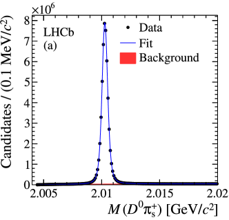
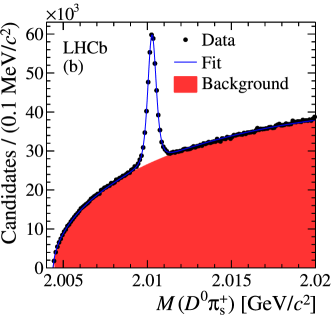
Figure 1: Distribution of $M(D^{0}\pi_{\rm s}^{+})$ for selected (a) right-sign $D^{0}\rightarrow K^{-}\pi^{+}$ and (b) wrong-sign $D^{0}\rightarrow K^{+}\pi^{-}$ candidates.

The RS and WS samples for $D^{0}$ and $\kern 1.99997pt\overline{\kern-1.99997ptD}{}^{0}$ mesons are each divided into 13 bins of $D^{0}$ decay time to compute decay-time-dependent WS-to-RS yield ratios. The ratios $R^{+}$ and $R^{-}$ observed in the $D^{0}$ and $\kern 1.99997pt\overline{\kern-1.99997ptD}{}^{0}$ samples and their differences are shown in Fig. 4. These are corrected for the relative efficiencies $\epsilon_{r}^{\pm}$ to account for charge asymmetries in reconstructing $K^{\mp}\pi^{\pm}$ final states. The relative efficiencies are measured from data using the efficiency ratio

$$\epsilon_{r}^{+}\equiv 1/\epsilon_{r}^{-}\equiv\frac{\epsilon(K^{+}\pi^{-})}{\epsilon(K^{-}\pi^{+})}=\frac{N(D^{-}\rightarrow K^{+}\pi^{-}\pi^{-})}{N(D^{+}\rightarrow K^{-}\pi^{+}\pi^{+})}\frac{N(D^{+}\rightarrow K^{0}_{\rm\scriptscriptstyle S}\pi^{+})}{N(D^{-}\rightarrow K^{0}_{\rm\scriptscriptstyle S}\pi^{-})}.$$ (4)

With the asymmetry between $D^{+}$ and $D^{-}$ production rates canceled in the ratio, the $D^{\pm}\rightarrow K^{\pm}\pi^{\mp}\pi^{\mp}$ events are properly weighted to match the kinematics of the $D^{\pm}\rightarrow K^{0}_{\rm\scriptscriptstyle S}\pi^{\pm}$ events. Similarly, these samples are weighted as functions of $K\pi$ momentum to match the RS momentum spectra. The charge asymmetry $A_{K\pi}\equiv(\epsilon_{r}^{+}-1)/(\epsilon_{r}^{+}+1)$ is found to be in the range $0.8$–$1.2\%$ with $0.2\%$ precision, and independent of decay time. Charm mesons produced in $b$-hardron decays (secondary $D$ decays) are assigned with wrong decay time, and could bias the measured WS-to-RS yield ratio. When the secondary component is not subtracted, the measured WS-to-RS yield ratio is written as $R(t)[1-\Delta_{B}(t)]$, where $R(t)$ is the ratio of the promptly produced candidates according to Eq. (1), and $\Delta_{B}(t)$ is a time-dependent bias due to the secondary contamination. Since $R(t)$ is measured to be monotonically non-decreasing [11], and the decay time for secondary decays is overestimated during reconstruction, $\Delta_{B}(t)$ can be bounded for all decay times as $0\leq\Delta_{B}(t)\leq f_{B}^{\mathrm{RS}}(t)\left[1-R_{D}/R(t)\right]$, where $f_{B}^{\mathrm{RS}}(t)$ is the fraction of secondary decays in the RS sample at decay time $t$ [16]. In this analysis, most of the secondary $D$ decays are removed by requiring the $\chi^{2}$ of $D^{0}$ impact parameter with respect to the primary vertex, $\chi^{2}(\mathrm{IP})$, to be smaller than 9. To determine the residual secondary decays, $f_{B}^{\mathrm{RS}}(t)$ is measured by fitting the $\chi^{2}(\mathrm{IP})$ distribution of the RS $D^{0}$ candidates in bins of decay time (see Fig. 2). The $\chi^{2}(\mathrm{IP})$ shape of the secondary component, and its dependence on decay time, is also determined from data by studying the sub-sample of candidates that are reconstructed, in combination with other tracks in the events, as $B\rightarrow D^{*}\mu X$. Figure 3 (a) shows the measured values of $f_{B}^{\mathrm{RS}}(t)$. We find that the secondary contamination is about 3% fraction of signals, and has negligible asymmetry when evaluated independently for $D^{0}$ and $\kern 1.99997pt\overline{\kern-1.99997ptD}{}^{0}$ decays.

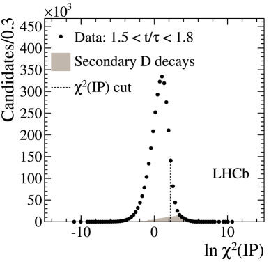
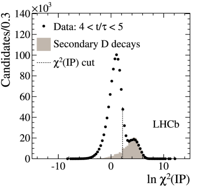
Figure 2: Background-subtracted distributions of $\chi^{2}_{\mathrm{IP}}$ for RS decays in two decay-time bins. The dashed line indicates the analysis selection requirement; the hatched histogram represents the estimated secondary component.

Peaking background in $M(D^{0}\pi_{\rm s}^{+})$, that is not accounted for in our mass fits, arises from $D^{*}$ decays for which the $\pi_{s}^{+}$ is correctly reconstructed, but the $D^{0}$ decay products are partially reconstructed or misidentified. This background is suppressed by the use of tight particle identification and $K\pi$ mass requirements. The dominant source of peaking background leaking into our signal region is from RS $K\pi$ events which are doubly misidentified as a WS candidate. This contamination is expected to have the same decay time dependence of RS decays and, if neglected, would marginally affect the determination of the mixing parameters, but lead to a small increase in the measured value of $R_{D}$. From the events in the $D^{0}$ mass sidebands, we derive a bound on the possible time dependence of this background (see Fig. 3 (b)). Contamination from peaking background due to partially reconstructed $D^{0}$ decays is found to be about 0.5% of the WS signal candidates, and has negligible asymmetry when evaluated independently for $D^{0}$ and $\kern 1.99997pt\overline{\kern-1.99997ptD}{}^{0}$ decays.

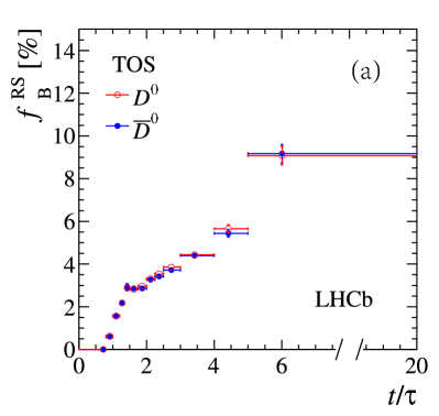
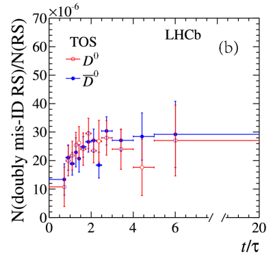
Figure 3: Decay-time evolution of the contamination from (a) secondary $D$ decays and (b) doubly misidentified RS candidates normalized to the RS signal yield, for the data that meet the hardware trigger requirement (TOS), separately for $D^{0}$ and $\kern 1.99997pt\overline{\kern-1.99997ptD}{}^{0}$ decays.

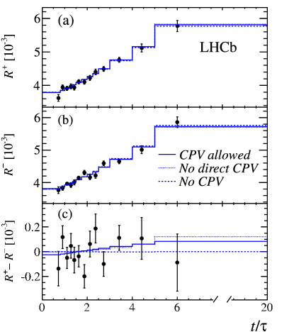
Figure 4: Efficiency-corrected ratios of WS-to-RS yields for (a) $D^{*+}$ decays, (b) $D^{*-}$ decays, and (c) their differences as functions of decay time in units of $D^{0}$ lifetime. Projections of fits allowing for (dashed line) no $C\!P$ violation, (dotted line) no direct $C\!P$ violation, and (solid line) full $C\!P$ violation are overlaid. The abscissa of the data points corresponds to the average decay time over the bin; the error bars indicate the statistical uncertainties.

Table 1: Results of fits to the data for different hypotheses on the $C\!P$ symmetry. The reported uncertainties include systematic effects.

Direct and indirect $CP$ violation				no direct $CP$ violation				no $CP$ violation
$R_{D}$ [	$10^{-3}$]	$3.568$ $\pm$	$0.066$	$R_{D}$ [	$10^{-3}$]	$3.568$ $\pm$	$0.066$	$R_{D}$ [	$10^{-3}$]	$3.568$ $\pm$	$0.066$
$A_{D}$ [	$10^{-2}$]	$-0.7$ $\pm$	$1.9$	$y^{\prime+}$ [	$10^{-3}$]	$\phantom{-}4.8$ $\pm$	$1.1$	$y^{\prime}$ [	$10^{-3}$]	$\phantom{-}4.8$ $\pm$	$1.0$
$y^{\prime+}$ [	$10^{-3}$]	$\phantom{-}5.1$ $\pm$	$1.4$	$x^{\prime 2+}$ [	$10^{-5}$]	$\phantom{-}6.4$ $\pm$	$5.5$	$x^{\prime 2}$ [	$10^{-5}$]	$\phantom{-}5.5$ $\pm$	$4.9$
$x^{\prime 2+}$ [	$10^{-5}$]	$\phantom{-}4.9$ $\pm$	$7.0$	$y^{\prime-}$ [	$10^{-3}$]	$\phantom{-}4.8$ $\pm$	$1.1$	$\chi^{2}/\text{ndf}$		$\;\;\;\;86.4/101$
$y^{\prime-}$ [	$10^{-3}$]	$\phantom{-}4.5$ $\pm$	$1.4$	$x^{\prime 2-}$ [	$10^{-5}$]	$\phantom{-}4.6$ $\pm$	$5.5$
$x^{\prime 2-}$ [	$10^{-5}$]	$\phantom{-}6.0$ $\pm$	$6.8$	$\chi^{2}/\text{ndf}$		$\;\;\;\;86.0/99$
$\chi^{2}/\text{ndf}$		$\;\;\;\;85.9/98$

Figure 4 shows that the WS-to-RS yield ratios from the data are fit three times. The first fit allows direct and indirect $C\!P$ violation, the second fit allows only indirect $C\!P$ violation by requiring a common value for $R_{D}$ in the $D^{0}$ and $\kern 1.99997pt\overline{\kern-1.99997ptD}{}^{0}$ samples, and the last fit is a $C\!P$-conserving fit that constrains all mixing parameters $(R_{D},\,x^{\prime 2},\,y^{\prime})$ to be the same in both samples. The fit $\chi^{2}$ accounts for systematic effects due to the decay-time evolution of the secondary $D$ decays and peaking background. The fit results are shown in Table 1 and Fig. 4, respectively. Figure 5 shows the central values and confidence regions in the $(x^{\prime 2},\,y^{\prime})$ plane. The data are compatible with $C\!P$ symmetry.

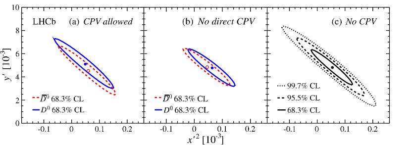
Figure 5: Two-dimensional confidence regions in the $(x^{\prime 2},y^{\prime})$ plane obtained (a) without any restriction on $C\!P$ violation, (b) assuming no direct $C\!P$ violation, and (c) assuming $C\!P$ conservation. The dashed (solid) curves in (a) and (b) indicate the contours of the mixing parameters associated with $\kern 1.79997pt\overline{\kern-1.79997ptD}{}^{0}$ ($D^{0}$) decays. The best-fit value for $\kern 1.79997pt\overline{\kern-1.79997ptD}{}^{0}$ ($D^{0}$) decays is shown with an open (filled) point. The solid, dashed, and dotted curves in (c) indicate the contours of $C\!P$-averaged mixing parameters at 68.3%, 95.5%, and 99.7% confidence levels (CL), respectively. The best-fit value is shown with a point.

From the fit results allowing for $C\!P$ violation, we build up a likelihood for $|q/p|$ using the relations of Eq. (2). Confidence intervals shown in Fig. 6 are derived with a likelihood-ratio ordering and assuming that the parameter correlations are independent of the true values of the mixing parameters. At the 68.3% CL, the magnitude of $q/p$ is determined to be $0.75<|q/p|<1.24$ when any $C\!P$ violation is allowed, and $0.91<|q/p|<1.31$ for the case without direct $C\!P$ violation. Figure 6 demonstrates the power of the present results on constraining $|q/p|$ and $\phi$, when combined with other available measurements. In the limit that direct $C\!P$ violation is negligible, and theoretical constraints such as the relationship $\phi=\tan^{-1}\left(\left(1-|q/p|^{2}\right)/\left(1+|q/p|^{2}\right)\right)$ [18, 19] are applicable, the constraints on $|q/p|$ will be even more stringent [11]. The capability of the present results on constraining $|q/p|$ is also suggested by directly looking at the slopes observed in Fig. 4. Indirect $C\!P$ violation results in a time dependence of the efficiency-corrected difference of WS-to-RS yield ratios. In the limit of negligible direct $C\!P$ violation, and $x^{\prime\pm}$, $y^{\prime\pm}$, and $\phi$ all very close to zero, as suggested in Eq. (2) the slopes of the WS-to-RS yield ratios (Fig. 4 (a) and (b)) and the slope in the difference of yield ratios (Fig. 4 (c)) are proportional to $y^{\prime}$ and $(|q/p|-|p/q|)y^{\prime}$, respectively. Within a span of about five decay-times, the slope in Fig. 4 (c) is about 5% of the individual slopes in Figs. 4 (a) and (b), and consistent with zero. Therefore, we expect $|q/p|$ to be constrained from one at a precision level of a few percent at most.

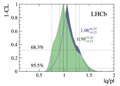
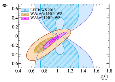
Figure 6: Left: (1 - CL) versus $|q/p|$ for the (green) direct and indirect $C\!P$ violation and (blue) no direct $C\!P$ violation fit results. The reported numbers correspond to the best-fit value and the uncertainties are computed using the respective 68.3% CL intervals. Right: 68.3% and 95.5% confidence regions with (blue) only the LHCb direct and indirect $C\!P$ violation allowed results, (brown) other measurements [11] excluding the LHCb WS results, (magenta) other measurements including the LHCb WS results. These confidence regions are in 1D, so that the projection to the $|q/p|$ axis reproduces the 1D intervals. The LHCb $A_{\Gamma}$ results [17] are not taken into consideration.

5 Summary

Using $D^{*+}\rightarrow D^{0}(\rightarrow K^{+}\pi^{-})\pi^{+}$ decays reconstructed in 3 $\mbox{\,fb}^{-1}$ of $pp$ collision data collected by the LHCb experiment in 2011–2012, $D^{0}$–$\kern 1.99997pt\overline{\kern-1.99997ptD}{}^{0}$ oscillation is studied with unprecedented level of precision. The observed mixing parameters $(R_{D},\,x^{\prime 2},\,y^{\prime})$ assuming $C\!P$ conservation are consistent with, $2.5$ times more precise than, and supersede the results based on a subset of the present data [12]. Studying $D^{0}$ and $\kern 1.99997pt\overline{\kern-1.99997ptD}{}^{0}$ decays separately shows no evidence for $C\!P$ violation and provides the most stringent bounds on the parameters $A_{D}$ and $|q/p|$ from a single experiment. The present LHCb $C\!P$ violation measurements also play an important role in constraining $|q/p|$ and $\phi$ when combined with other measurements [11].

ACKNOWLEDGEMENTS

We express our gratitude to our colleagues in the CERN accelerator departments for the excellent performance of the LHC. We thank the technical and administrative staff at the LHCb institutes. We acknowledge support from CERN and from the national agencies: CAPES, CNPq, FAPERJ and FINEP (Brazil); NSFC (China); CNRS/IN2P3 and Region Auvergne (France); BMBF, DFG, HGF and MPG (Germany); SFI (Ireland); INFN (Italy); FOM and NWO (The Netherlands); SCSR (Poland); MEN/IFA (Romania); MinES, Rosatom, RFBR and NRC “Kurchatov Institute” (Russia); MinECo, XuntaGal and GENCAT (Spain); SNSF and SER (Switzerland); NAS Ukraine (Ukraine); STFC (United Kingdom); NSF (USA). We also acknowledge the support received from the ERC under FP7. The Tier1 computing centres are supported by IN2P3 (France), KIT and BMBF (Germany), INFN (Italy), NWO and SURF (The Netherlands), PIC (Spain), GridPP (United Kingdom). We are thankful for the computing resources put at our disposal by Yandex LLC (Russia), as well as to the communities behind the multiple open source software packages that we depend on.

References

- [1] M. Artuso, B. Meadows and A. A. Petrov, Ann. Rev. Nucl. Part. Sci. 58, 249 (2008).
- [2] S. Bianco, F. L. Fabbri, D. Benson and I. Bigi, Riv. Nuovo Cim. 26N7, 1 (2003).
- [3] G. Burdman and I. Shipsey, Ann. Rev. Nucl. Part. Sci. 53, 431 (2003).
- [4] G. Blaylock, A. Seiden and Y. Nir, Phys. Lett. B 355, 555 (1995).
- [5] A. A. Petrov, Int. J. Mod. Phys. A 21, 5686 (2006).
- [6] E. Golowich, J. Hewett, S. Pakvasa and A. A. Petrov, Phys. Rev. D 76, 095009 (2007).
- [7] M. Ciuchini, E. Franco, D. Guadagnoli, V. Lubicz, M. Pierini, V. Porretti and L. Silvestrini, Phys. Lett. B 655, 162 (2007).
- [8] B. Aubert et al. [BaBar Collaboration], Phys. Rev. Lett. 98, 211802 (2007).
- [9] M. Staric et al. [Belle Collaboration], Phys. Rev. Lett. 98, 211803 (2007).
- [10] T. Aaltonen et al. [CDF Collaboration], Phys. Rev. Lett. 100, 121802 (2008).
- [11] Heavy Flavor Averaging Group, Y. Amhis et al., arXiv:1207.1158 [hep-ex], updated results and plots available at http://www.slac.stanford.edu/xorg/hfag/.
- [12] R. Aaij et al. [LHCb Collaboration], Phys. Rev. Lett. 110, 101802 (2013).
- [13] T. Aaltonen et al. [CDF Collaboration], arXiv:1309.4078 [hep-ex].
- [14] A. A. Alves, Jr. et al. [LHCb Collaboration], JINST 3, S08005 (2008).
- [15] R. Aaij et al. [LHCb Collaboration], arXiv:1309.6534 [hep-ex].
- [16] A. Di Canto, EPJ Web Conf. 49, 13009 (2013).
- [17] R. Aaij et al. [LHCb Collaboration], arXiv:1310.7201 [hep-ex].
- [18] Y. Grossman, Y. Nir and G. Perez, Phys. Rev. Lett. 103, 071602 (2009).
- [19] A. L. Kagan and M. D. Sokoloff, Phys. Rev. D 80, 076008 (2009).