Finite-Temperature Spectral Functions
from the Functional Renormalization Group

Abstract:

We present a method to obtain spectral functions at finite temperature from the Functional Renormalization Group. Our method is based on a thermodynamically consistent truncation of the flow equations for 2-point functions with analytically continued frequency components in the originally Euclidean external momenta. For the uniqueness of this continuation at finite temperature we furthermore implement the physical Baym-Mermin boundary conditions. Results are presented for mesonic spectral functions obtained from a two-flavor quark-meson model.

bluergb0,0,1 greenrgb0,1,0 redrgb1,0,0 REDrgb1,0,0

1 Introduction

The computation of real-time observables represents a common challenge within lattice calculations and other Euclidean approaches to Quantum Field Theory where an analytic continuation from imaginary to real time is needed for dynamic processes especially with timelike momentum transfer. This technical difficulty arises already in the vacuum but is even more severe at finite temperature where these continuations are based on discrete Matsubara frequencies and hence require additional boundary conditions for uniqueness [1, 2]. Even with the analytic structure completely fixed, however, the reconstruction of spectral functions from discrete numerical (i.e., noisy) data on Euclidean correlation functions, for example, is an ill-posed inverse problem. Maximum entropy methods (MEM) [3, 4, 5, 6, 7], Padé approximants [8, 9, 10, 11], or very recently also a standard Tikhonov regularization [12] have been proposed to deal with this problem. They all work best at low temperatures when the density of Matsubara modes is sufficiently large, but they all break down when the Euclidean input data is not sufficiently dense and precise.

Therefore any approach that can deal with the analytic continuation explicitly is highly desirable. In this work we employ the Functional Renormalization Group (FRG) which has proven very useful in nonperturbative applications in quantum field theory and statistical physics, see e.g. [13, 14, 15, 16, 17, 18, 19] for introductions. Within this framework the analytic continuation can be achieved already on the level of the flow equation, as proposed in [20, 21] and [22]. In addition to its simplicity our approach enjoys a number of particular advantages: First of all, it is thermodynamically consistent in that the spacelike limit of zero external momentum in the 2-point correlation functions agrees with the curvature or screening masses as extracted from the thermodynamic grand potential [20]. Secondly, it satisfies the physical Baym-Mermin boundary conditions at finite temperature [1] whose implementation here proceeds essentially as in a simple one-loop calculation [23]. Finally, although we focus on mesonic spectral functions obtained from the quark-meson model [24, 25] in this work it can be extended to calculate also quark and gluonic spectral functions as an alternative to analytically continued Dyson-Schwinger equations (DSEs) [26], or to using MEM on Euclidean FRG [27] or DSE results [28, 29, 30].

2 Flow Equations for the Quark-Meson Model

Within the FRG approach pioneered by Wetterich [31] the effective action is generalized to the scale dependent effective average action $\Gamma_{k}$ via the introduction of a regulator function $R_{k}$ which serves as an infrared (IR) regulator with an associated RG scale $k$. This regulator has then to be removed by taking $k$ from the ultraviolet (UV) cutoff scale $\Lambda$ down to zero. The scale dependence of the effective average action is governed by an exact one-loop equation involving full scale- and field-dependent propagators which takes the form

$$\partial_{k}\Gamma_{k}=\tfrac{1}{2}\mathrm{STr}{[}\partial_{k}R_{k}(\Gamma^{(2)}_{k}+R_{k})^{-1}{]},$$ (1)

where $\Gamma^{(2)}_{k}$ denotes the second functional derivative of the effective average action, and the supertrace includes internal and spacetime indices, the functional trace, typically in momentum space, and the minus sign with degeneracy factor for fermion loops, see Fig. 1 for a diagrammatic representation.

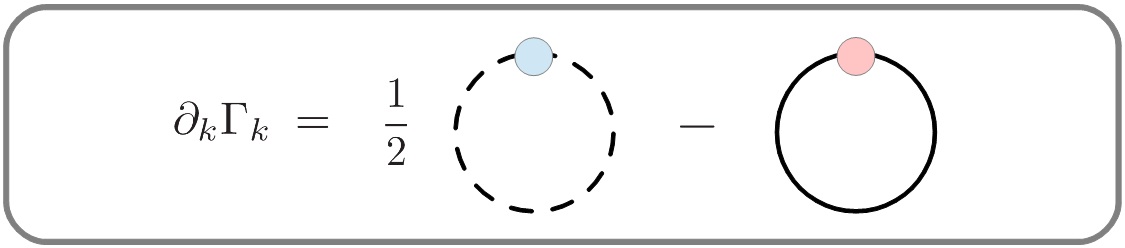
Figure 1: (color online) Diagrammatic representation of the flow equation for the effective action. Dashed (solid) lines represent bosonic (fermionic) propagators and circles the respective regulator insertions $\partial_{k}R_{k}$.

In the following we employ the quark-meson model, which serves as a low energy effective model for QCD with $N_{\text{f}}=2$ light quark flavors and yields the following Ansatz for the effective average action, in the lowest order derivative expansion where only the effective potential carries a scale dependence,

$$\Gamma_{k}[\bar{\psi},\psi,\phi]=\int d^{4}x\Big{\{}\bar{\psi}\left(\not{\partial}+h(\sigma+\mathrm{i}\vec{\tau}\cdot\vec{\pi}\gamma_{5})\right)\psi+\tfrac{1}{2}(\partial_{\mu}\vec{\phi})^{2}+U_{k}(\phi^{2})-c\sigma\Big{\}}\,,$$ (2)

with $\phi_{i}=(\sigma,\vec{\pi})_{i}$ and $\phi^{2}=\sigma^{2}+\vec{\pi}^{2}$. The effective potential $U_{k}(\phi^{2})$ allows for spontaneous breaking of chiral symmetry while the explicit breaking term $c\sigma$ accounts for a non-vanishing pion mass.

Inserting Eq. (2) into the flow equation for the effective action, Eq. (1), evaluated for constant fields and using the three-dimensional analogues of the LPA-optimized regulator functions [32], gives for the flow equation of the effective potential

$$\partial_{k}U_{k}=\tfrac{1}{2}I_{\sigma}^{(1)}+\tfrac{1}{2}(N-1)I_{\pi}^{(1)}-N_{\text{c}}N_{\text{f}}I_{\psi}^{(1)}.$$ (3)

Therein the loop functions $I_{\alpha}^{(i)}$ are defined as

$$I_{\alpha}^{(i)}=\mathrm{Tr}_{q}\left[\partial_{k}R_{k}(q)G_{\alpha,k}(q)^{i}\right],$$ (4)

with $\alpha\in\{\sigma,\pi,\psi\}$, $G_{\alpha,k}(q)$ the full (scale-dependent) Euclidean propagator and $R_{k}(q)$ chosen appropriately for bosonic and fermionic fields. The flow equations for the inverse mesonic 2-point functions are now obtained by taking two functional derivatives of Eq. (1),

$$\partial_{k}\Gamma^{(2)}_{\sigma,k} =J^{B}_{\sigma\sigma}(\Gamma_{\sigma\sigma\sigma}^{(0,3)})^{2}+(N-1)J^{B}_{\pi\pi}(\Gamma_{\sigma\pi\pi}^{(0,3)})^{2}-\tfrac{1}{2}I_{\sigma}^{(2)}\Gamma_{\sigma\sigma\sigma\sigma}^{(0,4)}-\tfrac{(N-1)}{2}I_{\pi}^{(2)}\Gamma_{\sigma\sigma\pi\pi}^{(0,4)}-2N_{\text{c}}N_{\text{f}}J^{F}_{\sigma},$$ (5)

$$\partial_{k}\Gamma^{(2)}_{\pi,k} =(J^{B}_{\sigma\pi}+J^{B}_{\pi\sigma})(\Gamma_{\sigma\pi\pi}^{(0,3)})^{2}-\tfrac{1}{2}I_{\sigma}^{(2)}\Gamma_{\sigma\sigma\pi\pi}^{(0,4)}-\tfrac{1}{2}I_{\pi}^{(2)}\!(\Gamma_{\pi\pi\pi\pi}^{(0,4)}+\!(N\!-\!2)\Gamma_{\pi\pi\tilde{\pi}\tilde{\pi}}^{(0,4)})-2N_{\text{c}}N_{\text{f}}J^{F}_{\pi},$$ (6)

with $\pi\neq\tilde{\pi}\in\{\pi_{1},\pi_{2},\pi_{3}\}$ and $N=4$ in our $O(4)$ case, see Fig. 2 for a graphical representation. The bosonic and fermionic loop functions are defined as

$$J^{B}_{\alpha\beta}(p)=\> \mathrm{Tr}_{q}\left[\partial_{k}R_{k}(q)G_{\alpha,k}(q-p)G_{\beta,k}(q)^{2}\right],$$ (7)

$$J^{F}_{\alpha}(p)=\> \mathrm{Tr}_{q}\left[\partial_{k}R_{k}(q)G_{\psi,k}(q)\Gamma_{\bar{\psi}\psi\alpha}^{(2,1)}G_{\psi,k}(q-p)\Gamma_{\bar{\psi}\psi\alpha}^{(2,1)}G_{\psi,k}(q)\right],$$ (8)

for $\alpha\in\{\sigma,\pi\}$ and at external momentum $p$. All vertices are taken to be momentum independent in our present truncation and are obtained by appropriate functional derivatives of the effective action for the quark-meson model, given by Eq. (2).

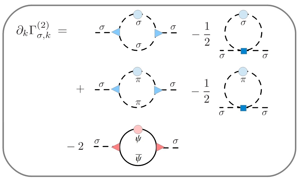
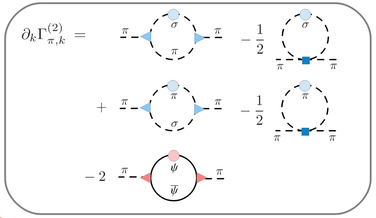
Figure 2: (color online) Diagrammatic representation of the flow equations for the inverse mesonic 2-point functions. Three-point vertices are represented by triangles, four-point vertices by squares.

3 Analytical Continuation and Numerical Implementation

We employ the following two-step procedure for the analytic continuation from imaginary to real time: Once the sum over the Matsubara frequencies in the flow equations for the 2-point functions is performed, we first exploit the periodicity of the bosonic and fermionic occupation numbers along the imaginary direction of the complex energy plane, i.e. with respect to discrete Euclidean external Matsubara modes $p_{0}=2n\pi T$,

$$n_{B,F}(E+\mathrm{i}p_{0})\rightarrow n_{B,F}(E),$$ (9)

cf. [37] for explicit expressions of the flow equations. In the second step, the retarded 2-point functions are then obtained from their Euclidean counterparts via the analytic continuation

$$\Gamma^{(2),R}(\omega,\vec{p})=\lim_{\epsilon\to 0}\Gamma^{(2),E}(p_{0}=-\mathrm{i}(\omega+\mathrm{i}\epsilon),\vec{p}),$$ (10)

where we keep a small but finite value of $\epsilon=1\,{\rm MeV}$ in our numerical implementation and consider the case of vanishing spatial momentum, $\vec{p}=0$. This substitution of the discrete Euclidean external $p_{0}$ by the continuous real frequency $\omega$ is done explicitly within the flow equation, before the integration of the RG scale $k$. Because of the one-loop structure of the flow equations together with the unregulated Matsubara sums, the correctness of this analytic continuation in the complex frequency plane follows directly from the corresponding one-loop formulae for the polarization functions in thermal field theory [23].

Finally, the spectral function is given by the discontinuity of the propagator and can hence be expressed in terms of the imaginary part of the retarded propagator as,

$$\rho(\omega)=-\frac{1}{\pi}\frac{\text{Im}\,\Gamma^{(2),R}(\omega)}{\left(\text{Re}\,\Gamma^{(2),R}(\omega)\right)^{2}+\left(\text{Im}\,\Gamma^{(2),R}(\omega)\right)^{2}}.$$ (11)

In order to numerically solve the flow equations for the effective potential and for the real and imaginary parts of the 2-point functions we take the effective potential at the UV scale to be of the form

$$U_{\Lambda}(\phi^{2})=\tfrac{1}{2}m_{\Lambda}^{2}\phi^{2}+\tfrac{1}{4}\lambda_{\Lambda}(\phi^{2})^{2}\,,$$ (12)

where the chosen values for the parameters and the corresponding values for observables in the IR are summarized in Table 1. For further details on our numerical implementation see [37].

$\Lambda$/MeV	$m_{\Lambda}/\Lambda$	$\lambda_{\Lambda}$	$c/\Lambda^{3}$	$h$	$f_{\pi}$/MeV	$m_{\pi}$/MeV	$m_{\sigma}$/MeV	$m_{\psi}$/MeV
1000	0.794	2.00	0.00175	3.2	93.5	137	509	299

Table 1: Employed parameter set and obtained vacuum values for observables in the IR, i.e. $k_{{\rm IR}}\approx 20\,{\rm MeV}$.

4 Results

Since the pion and sigma meson spectral functions are strongly affected by the possible decay processes, which in turn depend on the masses of the involved particles, we first turn to a discussion of the temperature-dependence of the meson screening masses and the quark mass, cf. Fig. 3. One clearly observes the expected crossover behavior with a pseudo-critical temperature of $T_{c}\approx 175\,{\rm MeV}$ as obtained from the maximum of the chiral susceptibility $\chi_{\sigma}\equiv 1/m_{\sigma}^{2}$, see [33, 34] and [35] for a comparison of different definitions of pseudo-critical temperatures. At higher temperatures the sigma and pion mass become degenerate, while the quark mass and the order parameter drastically decrease, indicating the progressing restoration of chiral symmetry.

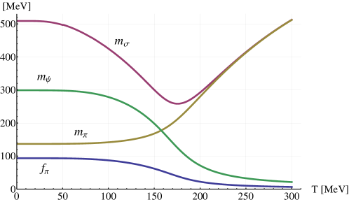
Figure 3: (color online) Meson masses, quark mass and chiral order parameter vs. temperature.

We now turn to a discussion of the pion and sigma meson spectral function which are shown as a function of external energy at different temperatures in Fig. 4. At $T=10\,{\rm MeV}$ the spectral functions closely resemble the vacuum structure already observed in previous studies, cf. [21, 36]. For external energies larger than $2m_{\psi}$ the decay of an (off-shell) pion into a quark anti-quark pair, ${\pi^{\prime}\rightarrow\bar{\psi}\psi}$, becomes energetically possible, giving rise to an increase of the pion spectral function at $\omega\geq 2m_{\psi}\approx 600\,{\rm MeV}$. The dominant channel affecting the sigma spectral function is the decay into two pions, ${\sigma^{\prime}\rightarrow\pi\pi}$, which is possible for $\omega\geq 2m_{\pi}$ and renders the sigma meson unstable.

At higher temperatures the process ${\pi^{\prime}\pi\rightarrow\sigma}$, which describes an off-shell pion and a pion of the heat bath going into a sigma meson, contributes to the pion spectral function for $\omega\leq m_{\sigma}-m_{\pi}$. At $T=150\,{\rm MeV}$ this results in modifications of $\rho_{\pi}$ near $\omega\approx 100\,{\rm MeV}$ while the sigma spectral function develops a sharp peak at $\omega\approx 280\,{\rm MeV}$, as expected near the chiral crossover, where neither the decay into two pions nor into two quarks is energetically possible. When increasing the temperature further, the quarks become the lightest degrees of freedom considered here, providing decay channels for both the pion and the sigma meson down to small external energies, leading to a broadening of the pronounced peaks in the spectral functions which eventually become degenerate.

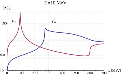
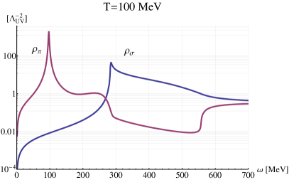
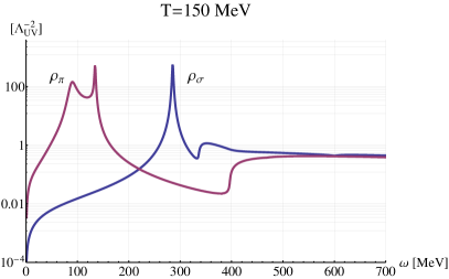
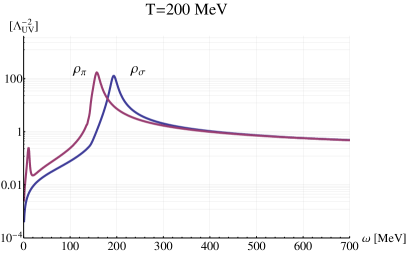
Figure 4: (color online) Sigma and pion spectral function vs. external energy at different temperatures.

5 Summary and Outlook

We have presented a method to obtain spectral functions at finite temperature from the Functional Renormalization Group, based on previous studies in the vacuum [21, 36]. The method involves an analytic continuation from imaginary time to real time performed on the level of the flow equations and has been illustrated here for mesonic spectral functions obtained from the quark-meson model. Our approach is comparably simple and can be extended in several ways, for example by including finite quark chemical potential which will allow to study spectral functions over the whole range of the phase diagram, including critical regimes, cf. [37]. Additionally, an extension to non-vanishing external spatial momenta is possible and will allow for the calculation of transport coefficients such as the shear viscosity.