On generalization of reversible second-order cellular automata

Abstract

A cellular automaton with $n$ states may be used for construction of reversible second-order cellular automaton with $n^{2}$ states. Reversible cellular automata with hidden parameters discussed in this paper are generalization of such construction and may have number of states $N=nm$ with arbitrary $m$. Further modification produces reversible cellular automata with reduced number of states $N^{\prime}<N=nm$.

1 Introduction

Second-order cellular automaton (CA) may be used for construction of reversible CA [1, 2]. The approach let us construct reversible CA with set of states $\mathsf{D}=\mathsf{S}\times\mathsf{S}\simeq\mathbb{Z}_{n^{2}}$ from arbitrary CA with states from some $\mathsf{S}\simeq\mathbb{Z}_{n}$. In the paper is suggested extension of such idea with $\mathsf{D}=\mathsf{S}\times\mathsf{H}\simeq\mathbb{Z}_{nm}$ with further reduction to some $\mathsf{R}\subset\mathsf{D}$. Here instead of second term $\mathsf{S}$ corresponding to previous state is used arbitrary set $\mathsf{H}$ considered as hidden parameter.

Some basic structures are introduced in Sec. 2, yet a preliminary acquaintance with properties of CA is supposed. The construction of reversible second-order CA is revisited in Sec. 3. Generalizations $\mathsf{D}=\mathsf{S}\times\mathsf{H}$ and $\mathsf{R}\subset\mathsf{D}$ are introduced in Sec. 4 and Sec. 5 respectively. Some examples are presented for clarification in Sec. 6.

2 Preliminaries

A space of cells $X$ is defined here in a general way as a finite or infinite discrete set. Simple examples of such spaces are $\mathbb{Z}^{d}$ and some subset of such lattices. Element $x\in X$ is called here location (of cell).

Set of states of each cell is a finite discrete set $\mathsf{S}$ with $n$ elements. A map $I_{\mathsf{S}}:{\mathsf{S}}\rightarrow\mathbb{Z}_{n}$ enumerates the states by indexes $0\ldots n-1$.

Complete description of each cell is a pair $(s,x)$ also denoted here as $(s)_{x}$ with $x\in X$, $s\in\mathsf{S}$. Configuration of whole CA is a map $\mathsf{S}^{X}:X\rightarrow\mathsf{S}$.

For a space of cells such as $X=\mathbb{Z}^{d}$ the neighborhood of given cell $\vec{x}\in\mathbb{Z}^{d}$ with $j$ adjacent cells is often described via shifts $(\vec{x}+\vec{\nu_{1}},\dots,\vec{x}+\vec{\nu_{j}})$ [2, 3], but for more general $X$ it should be defined as some function $\nu:X\rightarrow X^{j}$.

Local update rule is a function $f:\mathsf{S}^{j+1}\rightarrow\mathsf{S}$, where $(s,s_{1},\ldots,s_{j})\in\mathsf{S}^{j+1}$ is the vector of states for a neighborhood together with the cell itself. For a cell $(s)_{x}$ the notation $f[s]_{x}$ or $f[s]$ may be used for $f(s,s_{1},\ldots,s_{j})$.

Consideration of cellular automata on Penrose’s tilings [4] demonstrates that such a definition of neighborhood and local update rules may be still not enough to describe some models. The problem is not only varying number $j_{x}$ of adjacent cells, but also a few possible geometries and orientations of the neighborhood.

To include such models, let us use formal notation $[\mathsf{S}]$ for a domain of definition of local update rule. Element of such set is denoted here as $[s]\in[\mathsf{S}]$. In simplest case discussed above $[\mathsf{S}]=\mathsf{S}^{j+1}$, $[s]=(s,s_{1},\ldots,s_{j})$. For variable size of neighborhood it may be defined $[\mathsf{S}]=\bigcup_{k}\mathsf{S}^{j_{k}+1}$, $[s]=\bigl{(}k,(s,s_{1},\ldots,s_{j_{k}})\bigr{)}$.

For any location $x$ and each configuration $\mathsf{S}^{X}$ localization is a map

$$\Xi:(\mathsf{S}^{X},x)\rightarrow[\mathsf{S}].$$ (1)

The value of such a map for given $x$ is designated further as $[s]_{x}$ and for local update function may be used notation $f[s]$ or $f[s]_{x}$ already introduced earlier.

In simpler and more regular cases localization $\Xi$ of configuration $\mathsf{S}^{X}$ may be defined as composition of two maps. First map $\nu$ gives neighboring cells for given $x$. Localization $\mathsf{S}^{j+1}=[\mathsf{S}]$ is a restriction of configuration $\mathsf{S}^{X}$ to given neighborhood.

3 Second-order cellular automata

Let us consider arbitrary CA with set of states $\mathsf{S}=\mathbb{Z}_{n}$ and local update rule $f$. Second-order CA [1] produced from such a rule has the same set of locations $X$, but the state is a pair from set $\mathsf{D}=\mathsf{S}\times\mathsf{S}$ with $n^{2}$ elements and update rule is

$$f_{R}:(s,s^{\prime})\mapsto(f[s]\ominus s^{\prime},s),$$ (2)

where ‘$\ominus$’ is subtraction modulo $n$.

The update rule Eq. (2) may be decomposed into two reversible steps, an update:

$$f_{u}:(s,s^{\prime})\mapsto(s,f[s]\ominus s^{\prime})$$ (3)

and the swap:

$$w:(s,s^{\prime\prime})\mapsto(s^{\prime\prime},s).$$ (4)

The rule $f_{R}=w\,f_{u}$ is reversible $f_{R}^{-1}=f_{u}^{-1}w^{-1}$, where $w^{-1}=w$, $f_{u}^{-1}=f_{u}$.

The global reversibility of local operation $w$ Eq. (4) is rather obvious, because it acts on each cell separately. Operation $f_{u}$ Eq. (3) uses values of neighboring cells, but it acts only on second parameter of the state. Due to construction of the $f_{u}$ Eq. (3) neighboring cells are not affected by the second parameter (before application of $w$) and such a property produces global reversibility of $f_{u}$ in spite of the fact that definition Eq. (3) is local.

Generalization for less regular spaces $X$ with different configurations and number of neighboring cells is rather straightforward with localization $\Xi$ of configuration ${\mathsf{D}}^{X}$ Eq. (1). In fact, it is enough to consider localization $\Xi$ of ${\mathsf{S}}^{X}$ to construct $f_{u}$ Eq. (3) and swap $w$ only acts on cell itself.

4 Generalization with hidden parameters

The term second-order describes possibility to use information about previous state [1]. In local update rule such as Eq. (2) the information is accessible only to cell itself. It is possible to consider yet another interpretation of such update rules. The set of states is direct product of two components, but only one is accessible for neighboring cells.

Such alternative approach may be used for generalizations, if to consider the second component not as previous state, but as an arbitrary hidden parameter of a cell inaccessible for neighbors. In such a case size of both components may be different and instead of update Eq. (3) and exchange Eq. (4) could be used more general functions.

Let us consider CA with states from set of pairs $\mathsf{D}=\mathsf{S}\times\mathsf{H}$, $\mathsf{S}=\mathbb{Z}_{n}$, $\mathsf{H}=\mathbb{Z}_{m}$ and update rule represented as composition of two steps

$$f_{D}=\varpi f_{\upsilon}.$$ (5)

Here $\varpi$ is a fixed reversible transformation of $\mathsf{D}$ and

$$f_{\upsilon}:(s,h)\mapsto\bigl{(}s,F[s](h)\bigr{)},$$ (6)

where $F[s](h)=F(s,s_{1},\ldots,s_{j})(h)$ must be reversible function on set $\mathsf{H}$ for any vector of states $(s,s_{1},\ldots,s_{j})$.

In fact, not only second-order CA is particular case of such extension for $\mathsf{H}=\mathsf{S}$, but also arbitrary $n$-order CA may be considered in such a way with $\mathsf{H}=\mathsf{S}^{n-1}$ storing $n-1$ previous states and $\mathsf{D}=\mathsf{S}\times\mathsf{H}=\mathsf{S}^{n}$.

In most general case, reversible functions on $\mathsf{H}$ may be represented via transpositions $\pi_{m}$ of $m$ elements of $H$ and so instead of $f:\mathsf{S}^{j+1}\rightarrow\mathsf{S}$ (cf usual CA recollected in Sec. 2) should be used map $F$

$$F:\mathsf{S}^{j+1}\rightarrow\pi_{m}.$$ (7)

Only for set with two states both $\mathsf{S}=\mathbb{Z}_{2}$ and $\pi_{2}$ have two elements and such distinction is not essential.

Unlike the usual second-order CA discussed in Sec. 3 such an extended version is not necessary directly derived from some CA. On the other hand, it may be useful sometimes to start with a second-order CA and to consider local update rule with bigger number of output states Eq. (7). Simple example is discussed further in Sec. 6.2 for CA with three states.

Construction for spaces $X$ with variable number of neighboring cells is also straightforward due to localization $\Xi$ of configuration ${\mathsf{D}}^{X}$ Eq. (1). It is again enough to consider localization of ${\mathsf{S}}^{X}$ to construct $F$ Eq. (7) and $\varpi$ affects only state of cell itself.

5 Reduced number of states

Set with $nm$ states used above may be redundant. Reduction of previous construction on some subset $\mathsf{R}\subset\mathsf{S}\times\mathsf{H}$ is discussed below.

Let us consider some discrete set $\mathsf{R}$ with two projections $p_{1}:\mathsf{R}\rightarrow\mathsf{S}$ and $p_{2}:\mathsf{R}\rightarrow\mathsf{H}$. So, each state $r\in\mathsf{R}$ corresponds to pair $r\simeq\bigl{(}p_{1}(r),p_{2}(r)\bigr{)}$.

Figure 1: Scheme with reduced set of states

As an example, Fig. 1 with 12 states may be represented as set of pairs: $\{(0,0),(1,0),(2,0),(3,0),(4,0),\,(0,1),(1,1),(1,3),\,(0,2),(1,2),\,(0,3),\,(0,4)\}.$

Let us denote $m(s)$ number of states $r$ with $p_{1}(r)=s$, e.g., $m(0)=5$, $m(1)=3$, $m(2)=m(4)=1$, $m(3)=2$ for Fig. 1.

Due to representation of states from $\mathsf{R}$ via set of pairs it is possible again to use two-steps rule such as Eq. (5) with $\varpi$ is transposition on $\mathsf{R}$ and $f_{\upsilon}$ is an analogue of Eq. (6)

$$f_{\upsilon}:\bigl{(}p_{1}(r),p_{2}(r)\bigr{)}\mapsto\bigl{(}p_{1}(r),F[p_{1}(r)](p_{2}(r))\bigr{)},$$ (8)

where $F[p_{1}(r)]=F(p_{1}(r),p_{1}(r_{1}),\ldots,p_{1}(r_{j}))$ is reversible function (transposition) on set with $m(p_{1}(r))$ states. For example on Fig. 1 function $F[0]$ may exchange only five states $\{0,5,8,10,11\}$, $F[1]$ — $\{1,6,9\}$, etc. The $F$ depends only on $p_{1}$ projections of states in the neighborhood and rearranges states of the cell without change of $p_{1}$.

There is a formal difficulty in description of $F$ in Eq. (8). A map such as Eq. (7) may not be used directly, because value $m$ in $\pi_{m}$ for a state $r\in\mathsf{R}$ depends on $p_{1}(r)=s\in\mathsf{S}$.

A simple way to resolve such a problem — is to consider bigger formal set of states $\mathsf{S}\times\mathsf{H}\supset\mathsf{R}$, Fig. 2, but to use functions $F$ and $\varpi$ changing only states from $\mathsf{R}$. In such a case it is possible to use $F:\mathsf{S}^{j+1}\rightarrow\pi_{m_{\max}}$, where $m_{\max}\geq m(s)$ for any $s$.

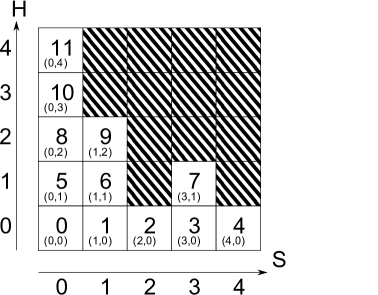
Figure 2: Reduced set of states $\mathsf{R}$ included into $\mathsf{S}\times\mathsf{H}$

Another method is to consider a family of functions

$$F_{s}:\mathsf{S}^{j}\rightarrow\pi_{m(s)}.$$ (9)

Here $\mathsf{S}^{j}$ is used instead of $\mathsf{S}^{j+1}$, because state of cell itself formally is not used as an argument of a function $F_{s}$ and is treated in a special way as an index inside of the family.

It is not necessary to introduce formal set $\mathsf{S}\times\mathsf{H}$ with auxiliary states in such a case. Such approach may also require an insignificant change of notation such as $F[s]=F_{s}(s_{1},\ldots,s_{j})$ instead of $F[s]=F(s,s_{1},\ldots,s_{j})$.

The construction of CA with variable number of neighboring cell may be again carried out with localization $\Xi$ of configuration ${\mathsf{R}}^{X}$ or $\mathsf{S}^{X}$ Eq. (1). It works both with formal consideration of $\mathsf{R}$ as a reduction of auxiliary space $\mathsf{S}\times\mathsf{H}$ and with definition of $\mathsf{R}$ via family of functions $F_{s}$.

6 Examples

6.1 CA with $2\times 2=4$ states

Let us consider two-states cellular automaton with transition function $f$. For two states there is no difference between subtraction and addition modulo two, the same binary operation is also known as XOR (eXclusive OR) and Eq. (2) may be written in more familiar way:

$$f_{R}:(s,s^{\prime})\mapsto(f[s]\mathop{\sf XOR}s^{\prime},s).$$ (10)

The Eq. (10) is transition function for reversible cellular automaton with four states Fig. 3.

Figure 3: Second order CA from CA with two states

The local transition function of initial CA may have only two values and they realize two possible reversible function on set with two elements Eq. (10)

$$\begin{array}[]{|c|c|c|}\hline\cr f&s^{\prime}&f\mathop{\sf XOR}s^{\prime}\\ \hline\cr\hline\cr 0&0&0\\ 0&1&1\\ \hline\cr 1&0&1\\ 1&1&0\\ \hline\cr\end{array}$$ (11)

With lack of other generalizations of function $f_{\upsilon}$ Eq. (6) for two states only $\varpi$ may be changed.

6.2 CA with $3\times 3=9$ states

Let us consider for comparison initial CA with three states.

$$f_{R}:(s,s^{\prime})\mapsto(f[s]+3-s^{\prime}\bmod 3,s).$$ (12)

The Eq. (12) is transition function for reversible cellular automaton with nine states Fig. 4.

Figure 4: Second order CA from CA with three states

Only three between six reversible transformations ($3!=6$) are represented in Eq. (12) and so it is possible to consider extensions with six different $f_{\upsilon}$ Eq. (6). For three states all six possible functions may be written quite naturally, e.g.

$$f_{0}(h) =h$$ (13a)

$$f_{1}(h) =h+1\bmod 3$$ (13b)

$$f_{2}(h) =h+2\bmod 3$$ (13c)

$$f_{3}(h) =3-h\bmod 3$$ (13d)

$$f_{4}(h) =4-h\bmod 3$$ (13e)

$$f_{5}(h) =2-h.$$ (13f)

It is clear, that only $f_{3}$, $f_{4}$ and $f_{5}$ are used in Eq. (12). Even without change of ‘swap’ function $\varpi$ there are possible extensions for such CA, due to possibility to associate six different actions Eq. (13) with local update rule instead of three. The inverse for $f_{3}$, $f_{4}$, $f_{5}$ and $f_{0}$ — is the function itself and $f^{-1}_{1}=f_{2}$.

6.3 Example of $\bm{\varpi}$ for CA with $3\times 2=6$ states

In examples above the operation $\varpi$ in Eq. (5) may simply exchange two components of the state because $\mathsf{H}=\mathsf{S}$. Such a swap for CA with $2\times 2$ states is shown on Fig. 5.

Figure 5: Swap operation $\varpi$ for $\mathsf{H}=\mathsf{S}$

Let us consider $3\times 2$ CA with six states, where $\mathsf{S}=(0,1,2)$, $\mathsf{H}=(0,1)$. An example of operation $\varpi$ for such CA is shown on Fig. 6.

Figure 6: Operation $\varpi$ for $3\times 2$ CA

6.4 CA with “blank” state

An example of application of constructions discussed in Sec. 5 is considered below. Let us start with some standard or extended second-order CA based on two-states CA such as Sec. 6.1.

It is useful sometimes to add special “blank” cells. A cellular space of CA may be restricted to some domain of arbitrary shape if to set all complementary cells to such “blank” value. Such a state may not be changed, but other states must be updated by the update function of initial CA without “blank” state.

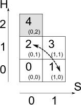
Figure 7: CA with “blank” state derived from second-order $2\times 2$ CA

On the Fig. 7 is shown extension of $2\times 2$ CA with “blank” state (4). The function $\varpi$ is denoted by arrows and exchanges only two states $(1\leftrightarrow 2)$, the function $f_{\upsilon}$ should be derived from initial CA and may change only first four states.

It should be mentioned, that term “reduced number of states” here should be treated with some care — given example could be formally described as reduction of CA with $6=2\times 3$ states, but it would not reflect properly idea of “blank” cells used for construction of the CA.

References

- [1] T. Toffoli and N. Margolus, “Invertible cellular automata: a review,” Physica D 45, 229–253 (1990).
- [2] S. Wolfram, Cellular automata and complexity: Collected papers, (Addison-Wesley, Reading MA 1994).
- [3] J. Kari and S. Taati, “Statistical mechanics of surjective cellular automata,” arXiv:1311.2319 [math] (2013).
- [4] N. Owens and S. Stepney, “Investigations of Game of Life cellular automata rules on Penrose tilings: lifetime and ash statistics,” Automata 2008, Bristol, UK pp. 1–-34 (Luniver Press, 2008).