Minimum $n$-Rank Approximation via Iterative Hard Thresholding

Abstract

The problem of recovering a low $n$-rank tensor is an extension of sparse recovery problem from the low dimensional space (matrix space) to the high dimensional space (tensor space) and has many applications in computer vision and graphics such as image inpainting and video inpainting. In this paper, we consider a new tensor recovery model, named as minimum $n$-rank approximation (MnRA), and propose an appropriate iterative hard thresholding algorithm with giving the upper bound of the $n$-rank in advance. The convergence analysis of the proposed algorithm is also presented. Particularly, we show that for the noiseless case, the linear convergence with rate $\frac{1}{2}$ can be obtained for the proposed algorithm under proper conditions. Additionally, combining an effective heuristic for determining $n$-rank, we can also apply the proposed algorithm to solve MnRA when $n$-rank is unknown in advance. Some preliminary numerical results on randomly generated and real low $n$-rank tensor completion problems are reported, which show the efficiency of the proposed algorithms. iterative hard thresholding; low-$n$-rank tensor recovery; tensor completion; compressed sensing

1 Introduction

The problem of recovering an unknown low-rank matrix $\hat{X}\in\mathbb{R}^{m\times n}$ from the linear constraint $\mathscr{A}(\hat{X})=\bm{b}$, where $\mathscr{A}:~{}\mathbb{R}^{m\times n}\rightarrow\mathbb{R}^{p}$ is the linear transformation and $\bm{b}\in\mathbb{R}^{p}$ is the measurement, has been an active topic of recent research with a range of applications including collaborative filtering (the Netflix probolem) (Goldberg et al., 1992), multi-task learning (Argyriou et al., 2008), system identification (Liu & Vandenberghe, 2009), and sensor localization (Biswas et al., 2006). One method to solve this inverse problem is to solve the matrix rank minimization problem:

$$\min_{X\in\mathbb{R}^{m\times n}}~{}\mbox{\rm rank}(X)\quad\mbox{\rm s.t.}\quad\mathscr{A}(X)={\bm{b}},$$ (1)

which becomes a mathematical task of minimizing the rank of $X$ such that it satisfies the linear constraint. With the application of nuclear norm which is the tightest convex approach to the rank function, one can relax the non-convex NP-hard problem (1) to a tractable, convex one (see Recht et al., 2010; Candès & Recht, 2009). An alternative model of this inverse problem is the minimum rank approximation problem:

$$\min_{X\in\mathbb{R}^{m\times n}}~{}\|\bm{b}-\mathscr{A}(X)\|_{2}\quad\mbox{\rm s.t.}\quad\mbox{\rm rank}(X)\leq r,$$ (2)

where $r=\mathrm{rank}(\hat{X})$ is known in advance, and $\hat{X}$ is the true data to be reconstructed. The model in (2) has been widely studied in the literature (see Haldar & Hernando, 2009; Keshavan et al., 2010; Lee & Bresler, 2010; Keshavan & Oh, 2009; Dai et al. & Kerman, 2011; Bresler & Lee, 2009). In fact, this formulation can not only work for the exact recovery case ($\mathscr{A}(\hat{X})=\bm{b}$), but also suit for the noisy case ($\bm{b}=\mathscr{A}(\hat{X})+\epsilon$), where $\epsilon$ denotes the noise by which the measurements are corrupted. Although the model (2) is based on a priori knowledge of the rank of $\hat{X}$, an incremental search over $r$, which increases the complexity of the solution by at most factor $r$, can be applied when the minimum rank $r$ is unknown. Particularly, if an upper bound on $r$ is available, we can use a bisection search over $r$ since the minimum of (2) is monotonously decreasing in $r$. Then the factor can reduce to $\log r$. Several effective algorithms based on (2) have been proposed, such as OPTSPACE (Keshavan & Oh, 2009), Space Evolution and Transfer (SET) (Dai et al. & Kerman, 2011), Atomic Decomposition for Minimum Rank Approximation (ADMiRA) (Lee & Bresler, 2010) and the Iterative Hard Thresholding (IHT) introduced in (Goldfarb & Ma, 2011). Among these algorithms, iterative hard thresholding algorithm is an easy-to-implement and fast method, which also shows the strong performance guarantees available with methods based on convex relaxation.

Recently, many researchers focus on the recovery problem in the high dimensional space, which has many applications in computer vision and graphics such as image inpainting (Bertalmío et al., 2000) and video inpainting. More specifically, by using the $n$-rank as a sparsity measure of a tensor (or multidimensional array), this inverse problem can be transformed into the mathematical task of recovering an unknown low $n$-rank tensor $\hat{\mathcal{X}}\in\mathbb{R}^{n_{1}\times\cdots\times n_{N}}$ from its linear measurements $\mathscr{A}(\hat{\mathcal{X}})=\bm{b}$ via a given linear transformation $\mathscr{A}:{\mathbb{R}}^{n_{1}\times n_{2}\times\ldots\times n_{N}}\rightarrow\mathbb{R}^{p}$ with $p\leq\prod^{N}_{i=1}n_{i}$. Some related works can be found in Gandy et al. (2011), Liu et al. (2009), Signoretto et al. (2010), Signoretto et al. (2013) and Yang et al. (2013). In all these studies, the authors mainly discussed the following tensor recovery model:

$$\min_{\mathcal{X}}~{}\sum_{i=1}^{N}w_{i}\mbox{\rm rank}({\mathcal{X}}_{<i>})\quad\mbox{\rm s.t.}\quad\mathscr{A}({\mathcal{X}})=\bm{b},$$ (3)

where $\mathcal{X}\in\mathbb{R}^{n_{1}\times\cdots\times n_{N}}$ is the decision variable, ${\mathcal{X}}_{<i>}$ is the mode-$i$ unfolding (the notation will be given in Section 2) of $\mathcal{X}$, $w_{i}$’s are the weighted parameters which satisfy $0\leq w_{i}\leq 1$ and $\sum_{i=1}^{N}w_{i}=1$. Note that (3) can be regarded as an extension of (1) in the high dimensional space ${\mathbb{R}}^{n_{1}\times n_{2}\times\ldots\times n_{N}}$ and it is a difficult non-convex problem due to the combination nature of the function rank($\cdot$). In order to solve it, the common method is replacing rank($\cdot$) by its convex envelope to get a convex tractable approximation and developing effective algorithms to solve the convex approximation, including FP-LRTC (fixed point continuation method for low $n$-rank tensor completion) (Yang et al., 2013), TENSOR-HC (hard completion) (Signoretto et al., 2013), and ADM-TR(E) (alternative direction method algorithm for low-$n$-rank tensor recovery) (Gandy et al., 2011). Additionally, Zhang & Huang (2012) investigated the exact recovery conditions for the low $n$-rank tensor recovery problems via its convex relaxation. And lately, (Goldfarb & Qin, 2014) studied the problem of robust low $n$-rank tensor recovery in a convex optimization framework, drawing upon recent advances in robust Principal Component Analysis and tensor completion.

In this paper, we consider a new alternative recovery model extended from problem (2), which is called as minimum $n$-rank approximation (MnRA):

$$\min_{\mathcal{X}\in\mathbb{R}^{n_{1}\times\cdots\times n_{N}}}~{}\|\mathscr{A}({\mathcal{X}})-\bm{b}\|^{2}_{2}\quad\mbox{\rm s.t.}\quad\mbox{\rm rank}({\mathcal{X}}_{<i>})\leq r_{i}~{}~{}\forall~{}i,$$ (4)

where $(r_{1},r_{2},\cdots,r_{N})$ is the $n$-rank of the ture data $\hat{\mathcal{X}}$ to be restored. Note that this formulation has not been discussed in tensor space in the literature to our knowledge and it also includes both the noisy case ($\mathscr{A}(\hat{\mathcal{X}})+\epsilon=\bm{b}$) and noiseless case ($\mathscr{A}(\hat{\mathcal{X}})=\bm{b}$). One of its special cases is the low $n$-rank tensor completion (LRTC) problem:

$$\min_{\mathcal{X}\in\mathbb{R}^{n_{1}\times\cdots\times n_{N}}}~{}\|\mathcal{X}_{\Omega}-\mathcal{M}_{\Omega}\|^{2}_{F}\quad\mbox{\rm s.t.}\quad\mbox{\rm rank}({\mathcal{X}}_{<i>})\leq r_{i}~{}~{}\forall~{}i,$$ (5)

where $\mathcal{X}$, $\mathcal{M}$ are $N$-way tensors with identical size in each mode, and $\mathcal{X}_{\Omega}$ (or $\mathcal{M}_{\Omega}$) denotes the tensor whose $(i_{1},i_{2},\cdots,i_{N})$-th component equal to $\mathcal{X}_{i_{1}i_{2}\cdots i_{N}}$ (or $\mathcal{M}_{i_{1}i_{2}\cdots i_{N}}$) if $(i_{1},i_{2},\cdots,i_{N})\in\Omega$ and zero otherwise. To solve (4), we propose an iterative hard thresholding algorithm, which is easy to implement and very fast. Particularly, we prove that for the noiseless case the iterative sequence generated by the proposed algorithm is globally linearly convergent to the true data $\hat{\mathcal{X}}$ with the rate $\frac{1}{2}$ under some conditions, while for the noisy case the distance between the iterative sequence and the true data $\hat{\mathcal{X}}$ is decreased quickly associated with the noise $\epsilon$. Additionally, combining an effective heuristic for determining $n$-rank, we can also apply the proposed algorithm to solve MnRA when $n$-rank of $\hat{\mathcal{X}}$ is unknown in advance. Some preliminary numerical results are reported and demonstrate the efficiency of the proposed algorithms.

The rest of our paper is organized as follows. In Section 2, we first briefly introduce some preliminary knowledge of tensor. Then, we propose an iterative hard thresholding algorithm to solve the minimum $n$-rank approximation problem in Section 3 and the convergence analysis of the proposed algorithm will be presented in Section 4. In Section 5 and Section 6, we give some implementation details and report some preliminary numerical results for low $n$-rank tensor completion, respectively. Conclusions are given in the last section.

2 Preliminary knowledge

In this section, we briefly introduce some essential nomenclatures and notations used in this paper; and more details can be found in Kolda & Bader (2009). Scalars are denoted by lowercase letters, e.g., $a,b,c,\cdots$; vectors by bold lowercase letters, e.g., $\bm{a},\bm{b},\bm{c},\cdots$; and matrices by uppercase letters, e.g., $A,B,C,\cdots$. An N-way tensor is denoted as $\mathcal{X}\in\mathbb{R}^{n_{1}\times\ldots\times n_{N}}$, whose elements are denoted as $x_{j_{1}\cdots j_{k}\cdots j_{N}}$, where $1\leqslant j_{k}\leqslant n_{k}$ and $1\leqslant k\leqslant N$. Let us denote tensor space by $\mathbb{T}$ for convenience, i.e., ${\mathbb{T}}:={\mathbb{R}}^{n_{1}\times n_{2}\times\ldots\times n_{N}}$. Then, for any ${\mathcal{X}},{\mathcal{Y}}\in{\mathbb{T}}$, the inner product is defined as

$$\langle{\mathcal{X}},{\mathcal{Y}}\rangle=\sum_{j_{1}=1}^{n_{1}}\sum_{j_{2}=1}^{n_{2}}\cdots\sum_{j_{N}=1}^{n_{N}}{\mathcal{X}}_{j_{1}j_{2}\ldots j_{N}}{\mathcal{Y}}_{j_{1}j_{2}\ldots j_{N}}.$$

Obviously, the tensor space ${\mathbb{T}}$ becomes a Hilbert space with the above definition of the inner product, and the corresponding Frobenius-norm is $\|{\mathcal{X}}\|_{F}=\sqrt{\langle{\mathcal{X}},{\mathcal{X}}\rangle}$.

The mode-$i$ fibers are all vectors $x_{j_{1}\ldots j_{i-1}:j_{i+1}\ldots j_{N}}$ obtained by fixing the indexes of $\{j_{1},\ldots j_{N}\}\backslash j_{i}$, which are analogue of matrix rows and columns. The mode-$i$ unfolding of ${\mathcal{X}}\in{\mathbb{T}}$, denoted by ${\mathcal{X}}_{<i>}$, arranges the mode-$i$ fibers to be the columns of the resulting matrix. The tensor element $(j_{1},j_{2},\ldots,j_{N})$ is mapped to the matrix element $(j_{i},l)$, where

$$l=1+\sum_{k=1,\;k\neq i}^{N}(j_{k}-1)L_{k}~{}~{}\mbox{\rm with}~{}~{}L_{k}=\prod_{j=1,\;j\neq i}^{k-1}n_{j},$$

which infers ${\mathcal{X}}_{<i>}\in\mathbb{R}^{n_{i}\times T_{i}}$, where $T_{i}=\prod_{k=1,k\neq i}^{N}n_{k}$. We also follow Gandy et al. (2011) to define the $n$-rank of a tensor ${\mathcal{X}}\in{\mathbb{T}}$ by

$$n\mathrm{-}\mbox{\rm rank}({\mathcal{X}})=(\mbox{\rm rank}({\mathcal{X}}_{<1>}),\mbox{\rm rank}({\mathcal{X}}_{<2>}),\cdots,\mbox{\rm rank}({\mathcal{X}}_{<N>})).$$

In the following parts of this paper, we say ${\mathcal{X}}$ is an ($r_{1},r_{2},...,r_{N}$)-rank tensor, if for any $i$, the rank of mode-$i$ unfolding of ${\mathcal{X}}$ is not greater than $r_{i}$, i.e., $\mbox{\rm rank}({\mathcal{X}}_{<i>})\leq r_{i}$ for all $i$. It should be pointed out that this definition is different from the notation of a “rank-($r_{1},r_{2},...,r_{N}$) tensor” in Lathauwer et al. (2000), which represents a tensor with the rank of each mode-$i$ unfolding is exactly $r_{i}$. The best ($r_{1},r_{2},...,r_{N}$)-rank approximation $\widetilde{{\mathcal{X}}}$ of a tensor ${\mathcal{X}}$ is defined as the following:

$$\widetilde{{\mathcal{X}}}=\arg\min\{\|{\mathcal{Y}}-{\mathcal{X}}\|_{F}:~{}{\mathcal{Y}}~{}\mbox{\rm is a (}r_{1},r_{2},...,r_{N}\mbox{\rm)-rank tensor}\}.$$

The $i$-mode (matrix) product of a tensor $\mathcal{X}\in\mathbb{R}^{n_{1}\times\cdots\times n_{N}}$ with a matrix $U\in\mathbb{R}^{L\times n_{i}}$ is denoted by $\mathcal{X}\times_{i}U$ and is of size $n_{1}\times\cdots\times n_{i-1}\times L\times n_{i+1}\times\cdots\times n_{N}$. It can be expressed in terms of unfolded tensors:

$$\mathcal{Y}=\mathcal{X}\times_{i}U\quad\Longleftrightarrow\quad Y_{<i>}=UX_{<i>}.$$

Additionally, for any transformation $\mathscr{A}$, $\|\mathscr{A}\|$ denotes the operator norm of the transformation $\mathscr{A}$; and for any vector $x$, we use Diag$(x)$ to denote a diagonal matrix with its $i$-th diagonal element being $x_{i}$.

3 Iterative hard thresholding for low $n$-rank tensor recovery

In this section, we will derive an iterative hard thresholding algorithm to solve problem (4). As a fast and efficient algorithm, iterative hard thresholding algorithm has been widely applied in various fields. Blumensath & Davies (2008) and Portilla (2009) first independently proposed the iterative hard thresholding algorithm to solve the compressed sensing recovery problem. Later, Blumensath and Davies presented a theoretical analysis of the iterative hard thresholding algorithm when applied to the compressed sensing recovery problem in Blumensath & Davies (2009). Through the analysis, they showed that the simple iterative hard thresholding algorithm has several good properties, including near-optimal error guarantees, robustness to observation noise, short memory requirement and low computational complexity. Also, it requires a fixed number of iterations and its performance guarantees are uniform. Recently, Blumensath (2012) used acceleration methods of choosing the step-size appropriately to improve the convergence speed of the iterative hard thresholding algorithm.

When it came to matrix space from vector space, Goldfarb & Ma (2011) studied the convergence/ recoverability properties of the fixed point continuation algorithm and its variants for matrix rank minimization. Particularly, in Goldfarb & Ma (2011), the authors proposed an iterative hard thresholdinging algorithm and discussed its convergence. At each iteration of their iterative hard thresholding algorithm, the authors first performed a gradient step

$$Y^{k+1}:=X^{k}-{\mathscr{A}}^{*}({\mathscr{A}}(X^{k})-\bm{b}),$$

where $X^{k}$ denotes the $k$-th iteration of $X$, $Y^{k+1}$ denotes the ($k+1$)-th iteration of $Y$ and ${\mathscr{A}}^{*}$ is the adjoint operator of ${\mathscr{A}}$ that is a linear transformation operating from $\mathbb{R}^{p}$ to $\mathbb{T}$. Then, they applied hard thresholding operator to the singular values of $Y^{k+1}$, i.e., they only kept the largest $r$ singular values of $Y^{k+1}$, to get $X^{k+1}$. It is easy to see that $X^{k+1}$ is actually the best $r$-rank approximation to $Y^{k+1}$. More specifically, by using $R_{r}(X)$ to denote the hard thresholding operator with threshold $r$ for $X$, the iterative scheme of their algorithm is as follows:

$$\left\{\begin{array}[]{l}Y^{k+1}=X^{k}-{\mathscr{A}}^{*}({\mathscr{A}}(X^{k})-\bm{b}),\\ X^{k+1}=R_{r}(Y^{k+1}).\end{array}\right.$$

Lately, in Kyrillidis & Cevher (2014), they studied acceleration schemes via memory-based techniques and randomized, $\epsilon$-approximate matrix projections to decrease the computational costs in the recovery process. In this paper, inspired by the work of Goldfarb & Ma (2011), we will develop an iterative hard thresholding algorithm for minimum $n$-rank approximation (4). In the following, we will do some theoretical analysis of problem (4) in order to derive the iterative scheme of our algorithm.

Firstly, we consider the objective function $f({\mathcal{X}}):=\|{\mathscr{A}}({\mathcal{X}})-\bm{b}\|_{2}^{2}$ in (4). Similar to that in Blumensath & Davies (2008), we introduce a surrogate objective function $F:~{}\mathbb{T}\otimes\mathbb{T}\otimes\cdots\otimes\mathbb{T}\rightarrow\mathbb{R}$ instead of function $f$:

$$\begin{array}[]{lc}F(\mathcal{Z}_{0},\mathcal{Z}_{1},\mathcal{Z}_{2},\ldots,\mathcal{Z}_{N})=\|\mathscr{A}(\mathcal{Z}_{0})-\bm{b}\|_{2}^{2}+\frac{1}{\tau}\sum\limits_{i=1}^{N}w_{i}\|\mathcal{Z}_{0}-\mathcal{Z}_{i}\|_{F}^{2}-\sum\limits_{i=1}^{N}w_{i}\|{\mathscr{A}}(\mathcal{Z}_{0})-{\mathscr{A}}({\mathcal{Z}}_{i})\|_{2}^{2},\end{array}$$ (8)

where $\tau>0$, $w_{i}\in[0,1]$, $\sum_{i=1}^{N}w_{i}=1$ and $\mathcal{Z}_{0},\mathcal{Z}_{1},\ldots,\mathcal{Z}_{N}\in\mathbb{T}$ are auxiliary variables in the domain of function $F$. It is obvious that $F({\mathcal{X}},{\mathcal{X}},\ldots,{\mathcal{X}})=f({\mathcal{X}})$ and if $\|\mathscr{A}\|^{2}\leq\frac{1}{\tau}$, $f({\mathcal{X}})\leq F({\mathcal{X}},\mathcal{Z}_{1},\mathcal{Z}_{2},\ldots$, $\mathcal{Z}_{N})$ for all ${\mathcal{X}}\in\mathbb{T}$, where $\|\mathscr{A}\|$ denotes the operator norm of linear operator $\mathscr{A}$. So, function $F$ is said to majorize $f$.

Let ${\mathcal{X}}^{k}$ be the $k$-th iteration and the $(k+1)$-th iteration ${\mathcal{X}}^{k+1}$ be the minimum of the function $F$ by setting its later $N$ variables to $X^{k}$, i.e., ${\mathcal{X}}^{k+1}=\mathop{\mathrm{argmin}}\limits_{\mathcal{X}}F({\mathcal{X}},{\mathcal{X}}^{k},{\mathcal{X}}^{k},\ldots,{\mathcal{X}}^{k})$. If $\|\mathscr{A}\|^{2}\leq\frac{1}{\tau}$, we have

$$f({\mathcal{X}}^{k+1}) = \|\mathscr{A}({\mathcal{X}}^{k+1})-\bm{b}\|_{2}^{2}$$

$$\leq \|\mathscr{A}({\mathcal{X}}^{k+1})-\bm{b}\|_{2}^{2}+(\frac{1}{\tau}\|{\mathcal{X}}^{k+1}-{\mathcal{X}}^{k}\|_{F}^{2}-\|{\mathscr{A}}({\mathcal{X}}^{k+1})-{\mathscr{A}}({\mathcal{X}}^{k})\|_{2}^{2})$$

$$= F({\mathcal{X}}^{k+1},{\mathcal{X}}^{k},{\mathcal{X}}^{k},...,{\mathcal{X}}^{k})$$

$$\leq F({\mathcal{X}}^{k},{\mathcal{X}}^{k},{\mathcal{X}}^{k},...,{\mathcal{X}}^{k})$$

$$= f({\mathcal{X}}^{k}),$$

where the first inequality follows from the assumption that $\|\mathscr{A}\|^{2}\leq\frac{1}{\tau}$, and the second inequality follows from that ${\mathcal{X}}^{k+1}$ is the minimum of $F({\mathcal{X}},{\mathcal{X}}^{k},{\mathcal{X}}^{k},\ldots,{\mathcal{X}}^{k})$. Thus, it can be clearly seen that if $\|\mathscr{A}\|^{2}\leq\frac{1}{\tau}$, fixing the latter $N$ variables in (8) and optimizing (8) with respect to the first variable will then decrease the value of the original objective function $f$. In other words, if $\|\mathscr{A}\|^{2}\leq\frac{1}{\tau}$, the iterative scheme solving problem (4) could be:

$${\mathcal{X}}^{k+1}=\mathop{\mathrm{argmin}}\limits_{\mathcal{X}\in\mathscr{C}}~{}F({\mathcal{X}},{\mathcal{X}}^{k},\ldots,{\mathcal{X}}^{k}),$$

where $\mathscr{C}$ denotes the set $\{\mathcal{X}|\mbox{\rm rank}(\mathcal{X}_{<i>})\leq r_{i},~{}i=1,2,\cdots,N\}$.

Note that, $F({\mathcal{X}},{\mathcal{X}}^{k},\ldots,{\mathcal{X}}^{k})$ can be written as:

$$\begin{array}[]{lc}F(\mathcal{X},\mathcal{X}^{k},\mathcal{X}^{k},...,\mathcal{X}^{k})=\frac{1}{\tau}\left(\|\mathcal{X}\|_{F}^{2}-2\langle\mathcal{X},\mathcal{X}^{k}-\tau\mathscr{A}^{*}(\mathscr{A}(\mathcal{X}^{k})-\bm{b})\rangle\right)\vspace{1mm}\\ ~{}~{}~{}~{}~{}~{}~{}~{}~{}~{}~{}~{}~{}~{}~{}~{}~{}~{}~{}~{}~{}~{}~{}~{}~{}~{}~{}~{}~{}~{}~{}~{}~{}~{}~{}~{}~{}~{}~{}~{}~{}~{}~{}~{}+\|\bm{b}\|_{2}^{2}-\|\mathscr{A}(\mathcal{X}^{k})\|_{2}^{2}-\frac{1}{\tau}\|\mathcal{X}^{k}\|_{F}^{2}.\end{array}$$

Then, it is easy to see that the solution of the following problem (without the constraints $\mbox{\rm rank}({\mathcal{X}}_{<i>})\leq r_{i}$ for any $i\in\{1,2,\cdots,N\}$):

$${\mathcal{X}}^{k+1}=\mathop{\mathrm{argmin}}\limits_{\mathcal{X}\in\mathbb{T}}~{}F({\mathcal{X}},{\mathcal{X}}^{k},\ldots,{\mathcal{X}}^{k})$$

is

$${\mathcal{X}}^{k+1}=\mathcal{X}^{k}-\tau\mathscr{A}^{*}(\mathscr{A}(\mathcal{X}^{k})-\bm{b}),$$

and the value of $F$ at this time is equal to

$$-\frac{1}{\tau}\|\mathcal{X}^{k+1}\|_{F}^{2}+\|\bm{b}\|_{2}^{2}-\|{\mathscr{A}}(\mathcal{X}^{k})\|_{2}^{2}-\frac{1}{\tau}\|\mathcal{X}^{k}\|_{F}^{2}.$$

Therefore, the minimum of $F(\mathcal{X},\mathcal{X}^{k},\mathcal{X}^{k},\ldots,\mathcal{X}^{k})$ with the constraints $\mbox{\rm rank}({\mathcal{X}}_{<i>})\leq r_{i}$ for any $i\in\{1,2,\cdots,N\}$ is then achieved at the best rank-$(r_{1},r_{2},...,r_{N})$ approximation of $\mathcal{X}^{k+1}$, i.e.,

$${\mathcal{X}}^{k+1}=\arg\min_{\mathcal{X}\in\mathscr{C}}F({\mathcal{X}},{\mathcal{X}}^{k},\ldots,{\mathcal{X}}^{k})=H_{r}\left(\mathcal{X}^{k}-\tau\mathscr{A}^{*}(\mathscr{A}(\mathcal{X}^{k})-\bm{b})\right),$$

where $H_{r}(\mathcal{Y})$ means the best rank-$(r_{1},r_{2},...,r_{N})$ approximation of $\mathcal{Y}$. However, for a tensor $\mathcal{Y}$, its best rank-$(r_{1},r_{2},...,r_{N})$ approximation is hard to be obtained in general. Thus, here we use another form to replace the exact best $(r_{1},r_{2},...,r_{N})$-rank approximation. Our method is first to compute the best rank-$r_{i}$ approximation of ${\mathcal{X}}^{k}_{<i>}$ for each $i$, then update $\mathcal{X}^{k+1}$ by the convex combination of the refoldings of these rank-$r_{i}$ matrices, i.e.,

$${\mathcal{X}^{k+1}}=\sum_{i=1}^{N}w_{i}\mathscr{B}_{i}^{*}(R_{r_{i}}(\mathscr{B}_{i}({\mathcal{X}^{k}}-\tau{\mathscr{A}}^{*}({\mathscr{A}}({\mathcal{X}}^{k})-\bm{b})))),$$ (10)

where ${\mathscr{B}}_{i}({\mathcal{X}})$ denotes the mode-$i$ unfolding of a tensor ${\mathcal{X}}\in{\mathbb{T}}$ for any $i\in\{1,2,\ldots,N\}$:

$${\mathscr{B}}_{i}:{\mathbb{T}}\rightarrow{\mathbb{R}}^{n_{i}\times J_{i}}~{}~{}\mathrm{with}~{}~{}{\mathscr{B}}_{i}({\mathcal{X}}):={\mathcal{X}}_{<i>},$$

and $\mathscr{B}_{i}^{*}$ denotes the adjoint operator of $\mathscr{B}_{i}$.

Now, we are ready to present the iterative hard thresholding algorithm for solving (4) as below and its convergence analysis will be presented in the next section.

Algorithm 3.1  Iterative hard thresholding for MnRA

Input: $\mathscr{A},~{}\mathbf{b},~{}\mathcal{X}^{0},~{}r_{i},~{}\tau$

while not converged, do

${\mathcal{Y}}^{k}={\mathcal{X}}^{k}-\tau{\mathscr{A}}^{*}({\mathscr{A}}({\mathcal{X}}^{k})-\bm{b})$

for $i=1:N$

$M_{i}^{k}=R_{r_{i}}(\mathscr{B}_{i}({\mathcal{Y}}^{k}))$

end

${\mathcal{X}}^{k+1}=\sum_{i=1}^{N}w_{i}\mathscr{B}_{i}^{*}(M_{i}^{k})$

end while

Output: $\mathcal{X}$

4 Convergence Results

In this section, we concentrate on the convergence of Algorithm 3.1. Let ${\bm{b}}={\mathscr{A}}({\mathcal{X}}^{*})$ with ${\mathcal{X}}^{*}\in\mathbb{T}$ being the true data to be restored, and it is known that ${\mathcal{X}}^{*}$ is an $(r_{1},r_{2},...,r_{N})$-rank tensor, i.e., the rank of the mode-$i$ unfolding of ${\mathcal{X}}^{*}$ is not greater than $r_{i}$ for each $i\in\{1,\ldots,N\}$. Algorithm 3.1 is used to recover the true data ${\mathcal{X}}^{*}$. Next, we will prove the following inequality to characterize the performance of the proposed algorithm:

$$\|{\mathcal{X}}^{*}-{\mathcal{X}}^{k+1}\|_{F}\leq\alpha\|{\mathcal{X}}^{*}-\mathcal{X}^{k}\|_{F},$$

where ${\mathcal{X}}^{k}$ denotes the $k$-th iteration generated by Algorithm 3.1 and $\alpha\in(0,1)$ denotes the rate at which the sequence converges to ${\mathcal{X}}^{*}$. The analysis begins by giving the following concepts, including the restricted isometry constant (RIC) of a linear transformation and singular value decomposition (SVD) basis of a matrix.

Definition 4.1 (Definition 1 in Shi et al. (2013)).

Let ${\bf r}=(r_{1},\ldots,r_{N})$. The restricted isometry constant $\delta_{\bf r}$ of a linear transformation ${\mathscr{A}}:\mathbb{T}$ $\rightarrow\mathbb{R}^{p}$ with order ${\bf r}$ is defined as the smallest constant such that

$$(1-\delta_{\bf r})\|\mathcal{X}\|_{F}^{2}\leq\|{\mathscr{A}}(\mathcal{X})\|_{2}^{2}\leq(1+\delta_{\bf r})\|\mathcal{X}\|_{F}^{2}$$ (11)

holds for any $(r_{1},\ldots,r_{N})$-rank tensor $\mathcal{X}$, i.e., rank$(\mathcal{X}_{<i>})\leq r_{i}$ for all $i\in\{1,\ldots,N\}$.

Definition 4.2 (Definition 2.5 in Goldfarb & Ma (2011)).

Assume that the $r$-rank matrix $X_{r}$ has the SVD $X_{r}=\sum_{i=1}^{r}\sigma_{i}{\bm{u}}_{i}{\bm{v}}_{i}^{\top}$. $\Gamma:=\{{\bm{u}}_{1}{\bm{v}}_{1}^{\top},{\bm{u}}_{2}{\bm{v}}_{2}^{\top},\cdots,{\bm{u}}_{r}{\bm{v}}_{r}^{\top}\}$ is called an SVD basis for the matrix $X_{r}$.

It’s easy to see that the elements in the subspace spanned by the SVD basis are all $r$-rank matrices. Based on these definitions, we give the following important lemma, which paves the way towards the convergence of Algorithm 3.1.

Lemma 4.3 (Lemma 4.1 in Goldfarb & Ma (2011)).

Suppose $X:=R_{r}(Y)$ is the best $r$-rank approximation to the matrix $Y$ and $\Gamma$ is an SVD basis of $X$. Then, for any $r$-rank matrix $X_{r}$ and SVD basis $\Gamma_{r}$ of $X_{r}$, we have

$$\|\mathcal{P}_{\mathbb{H}}(X)-\mathcal{P}_{\mathbb{H}}(Y)\|_{F}\leq\|\mathcal{P}_{\mathbb{H}}(X_{r})-\mathcal{P}_{\mathbb{H}}(Y)\|_{F},$$

where $\mathbb{H}$ is any orthonormal set of matrices satisfying $\mbox{\rm span}(\Gamma\cup\Gamma_{r})\subseteq\mbox{\rm span}(\mathbb{H})$, and $\mathcal{P}_{\mathbb{H}}(X)$ is the projection of $X$ onto the subspace spanned by $\mathbb{H}$..

Now we prove the convergence of Algorithm 3.1 under proper conditions.

Theorem 4.4.

Let ${\mathcal{X}}^{*}\in\mathbb{T}$ be the original data to be restored with ${\bm{b}}={\mathscr{A}}({\mathcal{X}}^{*})$, and ${\mathcal{X}}^{*}$ is an $(r_{1},r_{2},...,r_{N})$-rank tensor. Set $J_{i}=\lceil\frac{n_{i}}{r_{i}}\rceil$ and $J=\max\limits_{1\leq i\leq n}J_{i}$, where $\lceil\cdot\rceil$ means rounding up. Suppose that $\frac{3}{4}<\tau<\frac{5}{4}$, and let $\delta_{{\bf 3r}^{i}}$ be the RIC of ${\mathscr{A}}$ with order ${\bf 3r}^{i}=(n_{1},\ldots,n_{i-1},3r_{i},n_{i+1},\ldots,n_{N})$ and $\delta=\max\limits_{1\leq i\leq N}\delta_{{\bf 3r}^{i}}$. If $\delta<\frac{\frac{1}{4}-|1-\tau|}{\tau(1+\lceil\log_{2}J\rceil)}$, then the iterative sequence $\{{\mathcal{X}}^{k}\}$ generated by Algorithm 3.1 is linearly convergent to the original data ${\mathcal{X}}^{*}$ with rate $\frac{1}{2}$, i.e.,

$$\|{\mathcal{X}}^{*}-{\mathcal{X}}^{k+1}\|_{F}\leq\frac{1}{2}\|{\mathcal{X}}^{*}-\mathcal{X}^{k}\|_{F}.$$ (12)

Moreover, iterating the above inequality, we have

$$\|{\mathcal{X}}^{*}-{\mathcal{X}}^{k}\|_{F}\leq 2^{-k}\|{\mathcal{X}}^{*}-\mathcal{X}^{0}\|_{F}.$$

Proof 4.5.

To facilitate, we denote $X^{*}_{i}:=\mathscr{B}_{i}(\mathcal{X}^{*})$ and $X_{i}^{k}:=\mathscr{B}_{i}({\mathcal{X}}^{k})$ for all $i\in\{1,2...,N\}$ in the proof. Since ${\mathcal{X}}^{*}\in\mathbb{T}$ is a $(r_{1},r_{2},...,r_{N})$-rank tensor, we have $X^{*}_{i}$ is an $r_{i}$-rank matrix, i.e., the rank of $X^{*}_{i}$ is not greater than $r_{i}$. Note that from Algorithm 3.1, $M_{i}^{k}=R_{r_{i}}(\mathscr{B}_{i}({\mathcal{Y}}^{k}))$ is also an $r_{i}$-rank matrix for all $i\in\{1,2,\cdots,N\}$. Thus, for each $i\in\{1,2...,N\}$, there exist the SVD basises for $X^{*}_{i}$ and $M_{i}^{k}$, denoted by $\Gamma_{i}^{*}$ and $\Gamma_{i}^{k}$, respectively. And let $\mathbb{H}_{i}^{k}$ denote an orthonormal basis of the subspace span$(\Gamma_{i}^{*}\cup\Gamma_{i}^{k})$. Then the subspace spanned by $\mathbb{H}_{i}^{k}$, containing $X^{*}_{i}$ and $M_{i}^{k}$, is a set of $2r_{i}$-rank matrices. Setting $\mathcal{P}_{\mathbb{H}_{i}^{k}}(Z)$ to be the projection of $Z$ onto the subspace spanned by $\mathbb{H}_{i}^{k}$. Then, $\mbox{\rm rank}(\mathcal{P}_{\mathbb{H}_{i}^{k}}(Z))\leq 2r_{i}$.

Based on the aforementioned notations and the iterative scheme of Algorithm 3.1, we have

$$\|{\mathcal{X}}^{*}-{\mathcal{X}}^{k+1}\|_{F}=\|{\mathcal{X}}^{*}-\sum_{i=1}^{N}w_{i}\mathscr{B}_{i}^{*}(M_{i}^{k})\|_{F}$$ (13)

$$\leq \sum_{i=1}^{N}w_{i}\|X^{*}_{i}-M_{i}^{k}\|_{F}=\sum_{i=1}^{N}w_{i}\|\mathcal{P}_{\mathbb{H}_{i}^{k}}(X^{*}_{i})-\mathcal{P}_{\mathbb{H}_{i}^{k}}(M_{i}^{k})\|_{F}$$

$$\leq \sum_{i=1}^{N}w_{i}\left(\|\mathcal{P}_{\mathbb{H}_{i}^{k}}(X^{*}_{i})-\mathcal{P}_{\mathbb{H}_{i}^{k}}(\mathscr{B}_{i}({\mathcal{Y}}^{k}))\|_{F}+\|\mathcal{P}_{\mathbb{H}_{i}^{k}}(\mathscr{B}_{i}({\mathcal{Y}}^{k}))-\mathcal{P}_{\mathbb{H}_{i}^{k}}(M_{i}^{k})\|_{F}\right)$$

$$\leq 2\sum_{i=1}^{N}w_{i}\|\mathcal{P}_{\mathbb{H}_{i}^{k}}(X^{*}_{i})-\mathcal{P}_{\mathbb{H}_{i}^{k}}(\mathscr{B}_{i}({\mathcal{Y}}^{k}))\|_{F},$$

where the first and third inequality follow from the triangle inequality, the second equality follows from $X^{*}_{i},M_{i}^{k}\in\mbox{\rm span}(\mathbb{H}_{i}^{k})$, and the last inequality follows from Lemma 4.3. Furthermore, for each index $i\in\{1,2...,N\}$, we have

$$\|\mathcal{P}_{\mathbb{H}_{i}^{k}}(X^{*}_{i})-\mathcal{P}_{\mathbb{H}_{i}^{k}}(\mathscr{B}_{i}({\mathcal{Y}}^{k}))\|_{F}$$ (14)

$$= \|\mathcal{P}_{\mathbb{H}_{i}^{k}}(X^{*}_{i})-\mathcal{P}_{\mathbb{H}_{i}^{k}}(X_{i}^{k}-\tau\mathscr{B}_{i}{\mathscr{A}}^{*}({\mathscr{A}}({\mathcal{X}}^{k})-{\bm{b}}))\|_{F}$$

$$= \|\mathcal{P}_{\mathbb{H}_{i}^{k}}(X^{*}_{i}-X_{i}^{k})-\tau\mathcal{P}_{\mathbb{H}_{i}^{k}}\mathscr{B}_{i}{\mathscr{A}}^{*}{\mathscr{A}}\mathscr{B}_{i}^{*}(X^{*}_{i}-X_{i}^{k})\|_{F}$$

$$\leq |1-\tau|\|\mathcal{P}_{\mathbb{H}_{i}^{k}}(X^{*}_{i}-X_{i}^{k})\|_{F}+\tau\|(I-\mathcal{P}_{\mathbb{H}_{i}^{k}}\mathscr{B}_{i}{\mathscr{A}}^{*}{\mathscr{A}}\mathscr{B}_{i}^{*}\mathcal{P}_{\mathbb{H}_{i}^{k}})(X^{*}_{i}-X_{i}^{k})\|_{F}$$

$$+\tau\|\mathcal{P}_{\mathbb{H}_{i}^{k}}\mathscr{B}_{i}{\mathscr{A}}^{*}{\mathscr{A}}\mathscr{B}_{i}^{*}(I-\mathcal{P}_{\mathbb{H}_{i}^{k}})(X^{*}_{i}-X_{i}^{k})\|_{F}.$$

Therefore, in order to prove (12), i.e., $\|{\mathcal{X}}^{*}-{\mathcal{X}}^{k+1}\|_{F}\leq\frac{1}{2}\|{\mathcal{X}}^{*}-\mathcal{X}^{k}\|_{F}$, we need to estimate the upper bounds of the three terms in the right-hand side of (14), respectively. The specifical analysis is as follows:

• (Estimation on the upper bound of the term $|1-\tau|\|\mathcal{P}_{\mathbb{H}_{i}^{k}}(X^{*}_{i}-X_{i}^{k})\|_{F}$)

  Utilizing the non-expansion of projection operator, it’s simple to estimate an upper bound of term $\|\mathcal{P}_{\mathbb{H}_{i}^{k}}(X^{*}_{i}-X_{i}^{k})\|_{F}$ in the right-hand side of (14). This is given by

  $$|1-\tau|\|\mathcal{P}_{\mathbb{H}_{i}^{k}}(X^{*}_{i}-X_{i}^{k})\|_{F}\leq|1-\tau|\|X^{*}_{i}-X_{i}^{k}\|_{F}=|1-\tau|\|\mathcal{X}^{*}-\mathcal{X}^{k}\|_{F}.$$ (15)

• (Estimation on the upper bound of $\tau\|(I-\mathcal{P}_{\mathbb{H}_{i}^{k}}\mathscr{B}_{i}{\mathscr{A}}^{*}{\mathscr{A}}\mathscr{B}_{i}^{*}\mathcal{P}_{\mathbb{H}_{i}^{k}})(X^{*}_{i}-X_{i}^{k})\|_{F}$)

  Note that, for any matrix $Z\in\mbox{\rm span}({\mathbb{H}_{i}^{k}})$ with appropriate size, $\mbox{\rm rank}(\mathcal{P}_{\mathbb{H}_{i}^{k}}(Z))\leq 2r_{i}$. Thus, $\mathscr{B}_{i}^{*}\mathcal{P}_{\mathbb{H}_{i}^{k}}(Z)$ is a ${\bf 2r}^{i}$-rank tensor, where ${\bf 2r}^{i}=(n_{1},\ldots,n_{i-1},2r_{i},n_{i+1},\ldots,n_{N})$. Then, based on (4.1),

  $$(1-\delta_{{\bf 2r}^{i}})\|\mathscr{B}_{i}^{*}\mathcal{P}_{\mathbb{H}_{i}^{k}}(Z)\|_{F}^{2}\leq\|\mathscr{A}\mathscr{B}_{i}^{*}\mathcal{P}_{\mathbb{H}_{i}^{k}}(Z)\|_{F}^{2}\leq(1+\delta_{{\bf 2r}^{i}})\|\mathscr{B}_{i}^{*}\mathcal{P}_{\mathbb{H}_{i}^{k}}(Z)\|_{F}^{2},$$

  which implies that

  $$(1-\delta_{{\bf 2r}^{i}})\|\mathcal{P}_{\mathbb{H}_{i}^{k}}(Z)\|_{F}\leq\|\mathcal{P}_{\mathbb{H}_{i}^{k}}(\mathscr{B}_{i}\mathscr{A}^{*}\mathscr{A}\mathscr{B}_{i}^{*}\mathcal{P}_{\mathbb{H}_{i}^{k}}(Z))\|_{F}\leq(1+\delta_{{\bf 2r}^{i}})\|\mathcal{P}_{\mathbb{H}_{i}^{k}}(Z)\|_{F}.$$

  Therefore, we can obtain that

  $$\tau\|(I-\mathcal{P}_{\mathbb{H}_{i}^{k}}\mathscr{B}_{i}{\mathscr{A}}^{*}{\mathscr{A}}\mathscr{B}_{i}^{*}\mathcal{P}_{\mathbb{H}_{i}^{k}})(X^{*}_{i}-X_{i}^{k})\|_{F}\leq\tau\delta_{{\bf 2r}^{i}}\|X^{*}_{i}-X_{i}^{k}\|_{F}=\tau\delta_{{\bf 2r}^{i}}\|\mathcal{X}^{*}-\mathcal{X}^{k}\|_{F}.$$ (16)

• (Estimation on the upper bound of $\tau\|\mathcal{P}_{\mathbb{H}_{i}^{k}}(\mathscr{B}_{i}{\mathscr{A}}^{*}{\mathscr{A}}\mathscr{B}_{i}^{*}(I-\mathcal{P}_{\mathbb{H}_{i}^{k}})(X^{*}_{i}-X_{i}^{k}))\|_{F}$)

  Let the SVD of $X^{*}_{i}-X_{i}^{k}$ be $X^{*}_{i}-X_{i}^{k}=U\mathrm{Diag}(\sigma)V^{\top}$, where $\sigma=(\sigma_{1},\cdots,\sigma_{m-r_{i}})^{\top}$ is the vector of the singular values of $X^{*}_{i}-X_{i}^{k}$ with $\sigma_{1}\geq\cdots\geq\sigma_{m-r_{i}}\geq 0$. We decompose $\sigma$ into a sum of vectors $\sigma_{T_{l}}\;(l=1,2,\cdots)$, where disjoint index sets $T_{1}\cup T_{2}\cup\cdots\cup T_{J}=\{1,2,\cdots,m-r_{i}\}$ and the sparsity of each $T_{l}$ is $r_{i}$ (except possibly $T_{J}$). Then, $Z_{T_{1}}$ is the part of $X^{*}_{i}-X_{i}^{k}$ corresponding to the $r_{i}$ largest singular values, $Z_{T_{2}}$ is the part corresponding to the next $r_{i}$ largest singular values, and so on. Thus, we have $X^{*}_{i}-X_{i}^{k}=U(\sum_{l=1}^{J_{i}}Z_{T_{l}}^{k})V^{\top}$, where $Z_{T_{l}}^{k}$ is an $r_{i}$-rank matrix, $\|\mathscr{B}_{i}({\mathcal{X}}^{*}-\mathcal{X}^{k})\|_{F}^{2}=\sum_{l=1}^{J_{i}}\|Z_{T_{l}}^{k}\|_{F}^{2}$, and $J_{i}=\lceil\frac{n_{i}}{r_{i}}\rceil$. Then, we have

  $$\tau\|\mathcal{P}_{\mathbb{H}_{i}^{k}}(\mathscr{B}_{i}{\mathscr{A}}^{*}{\mathscr{A}}\mathscr{B}_{i}^{*}(I-\mathcal{P}_{\mathbb{H}_{i}^{k}})(X^{*}_{i}-X_{i}^{k}))\|_{F}$$ (17)

  $$\leq \tau\sum_{l=1}^{J_{i}}\|\mathcal{P}_{\mathbb{H}_{i}^{k}}(\mathscr{B}_{i}{\mathscr{A}}^{*}{\mathscr{A}}\mathscr{B}_{i}^{*}(I-\mathcal{P}_{\mathbb{H}_{i}^{k}})(Z_{T_{l}}^{k}))\|_{F}$$

  $$\leq \tau\delta_{{\bf 3r}^{i}}\sum_{l=1}^{J_{i}}\|(I-\mathcal{P}_{\mathbb{H}_{i}^{k}})Z_{T_{l}}^{k}\|_{F}$$

  $$\leq \tau\delta_{{\bf 3r}^{i}}\lceil\log_{2}{J_{i}}\rceil\|{\mathcal{X}}^{*}-\mathcal{X}^{k}\|_{F},$$

  where the first inequality follows from the triangle inequality, and the second inequality follows from the following facts:

  $$\|\mathcal{P}_{\mathbb{H}_{i}^{k}}(\mathscr{B}_{i}{\mathscr{A}}^{*}{\mathscr{A}}\mathscr{B}_{i}^{*}(I-\mathcal{P}_{\mathbb{H}_{i}^{k}})(Z_{T_{l}}^{k}))\|_{F}$$

  $$= \max_{\|W\|_{F}=1}\langle W,\mathcal{P}_{\mathbb{H}_{i}^{k}}(\mathscr{B}_{i}{\mathscr{A}}^{*}{\mathscr{A}}\mathscr{B}_{i}^{*}(I-\mathcal{P}_{\mathbb{H}_{i}^{k}})(Z_{T_{l}}^{k}))\rangle$$

  $$= \max_{\|W\|_{F}=1}\langle{\mathscr{A}}\mathscr{B}_{i}^{*}\mathcal{P}_{\mathbb{H}_{i}^{k}}(W),{\mathscr{A}}\mathscr{B}_{i}^{*}(I-\mathcal{P}_{\mathbb{H}_{i}^{k}})(Z_{T_{l}}^{k}))\rangle$$

  $$\leq \max_{\|W\|_{F}=1}\delta_{{\bf 3r}^{i}}\|W\|_{F}\|Z_{T_{l}}^{k}\|_{F}$$

  $$= \delta_{{\bf 3r}^{i}}\|Z_{T_{l}}^{k}\|_{F},$$

Therefore, by utilizing the results of items (a), (b), and (c), i.e., by combining (15), (16) and (17), we can further obtain that for each index $i\in\{1,2...,N\}$

$$\|\mathcal{P}_{\mathbb{H}_{i}^{k}}(X^{*}_{i})-\mathcal{P}_{\mathbb{H}_{i}^{k}}(\mathscr{B}_{i}({\mathcal{Y}}^{k}))\|_{F}\leq(|1-\tau|+\tau\delta_{{\bf 2r}^{i}}+\tau\delta_{{\bf 3r}^{i}}\lceil\log_{2}{J_{i}}\rceil)\|{\mathcal{X}}^{*}-\mathcal{X}^{k}\|_{F}.$$ (18)

Then, let $J=\max\limits_{1\leq i\leq n}J_{i}$ and $\delta=\max\limits_{1\leq i\leq N}\delta_{{\bf 3r}^{i}}$. Substituting (18) into (13), we have

$$\|{\mathcal{X}}^{*}-{\mathcal{X}}^{k+1}\|_{F} \leq 2\sum_{i=1}^{N}w_{i}\|\mathcal{P}_{\mathbb{H}_{i}^{k}}(X^{*}_{i})-\mathcal{P}_{\mathbb{H}_{i}^{k}}(\mathscr{B}_{i}({\mathcal{Y}}^{k}))\|_{F}$$ (19)

$$\leq 2(\tau\delta+\tau\delta\lceil\log_{2}{J}\rceil+|1-\tau|)\|{\mathcal{X}}^{*}-\mathcal{X}^{k}\|_{F},$$

where the second inequality follows from that fact that $\delta_{{\bf 2r}^{i}}\leq\delta_{{\bf 3r}^{i}}$ for all $i$.

By the assumption that $\delta<\frac{\frac{1}{4}-|1-\tau|}{\tau(1+\lceil\log_{2}J\rceil)}$, we have

$$\|{\mathcal{X}}^{*}-{\mathcal{X}}^{k+1}\|_{F}\leq\frac{1}{2}\|{\mathcal{X}}^{*}-\mathcal{X}^{k}\|_{F}.$$ (20)

Iterating this inequality, we obtain

$$\|{\mathcal{X}}^{*}-{\mathcal{X}}^{k}\|_{F}\leq 2^{-k}\|{\mathcal{X}}^{*}-\mathcal{X}^{0}\|_{F}.$$

The proof is complete.

Remark: Note that we use a parameter $\tau>0$ as the step-size in Algorithm 3.1. Actually, $\tau$ is scoped. In the conditions of Theorem 4.4, we assume $\frac{3}{4}<\tau<\frac{5}{4}$ to ensure that $\frac{\frac{1}{4}-|1-\tau|}{\tau(1+\lceil\log_{2}J\rceil)}>0$, since $\delta>0$. Actually, observing (19) given in the proof of Theorem 4.4, in order to ensure the convergence of the iterative sequence, we only need $2(\tau\delta+\tau\delta\lceil\log_{2}{J}\rceil+||1-\tau|)<1$, which implies that $\delta<\frac{\frac{1}{2}-|1-\tau|}{\tau(1+\lceil\log_{2}J\rceil)}$. Thus, $\delta>0$ implies that $\frac{1}{2}<\tau<\frac{3}{2}$, which is enough to guarantee the convergence of Algorithm 3.1.

Note that Theorem 4.4 considers the exact recovery case. However, it is possible to apply Algorithm 3.1 to recover the data corrupted by noise. Next, we will give the recoverability result of Algorithm 3.1 for the noisy case.

Theorem 4.6.

Let ${\mathcal{X}}^{*}\in\mathbb{T}$ be the original data to be restored with ${\bm{b}}={\mathscr{A}}({\mathcal{X}}^{*})+\epsilon$, where $\epsilon\in\mathbb{R}^{p}$ denotes the noise, and ${\mathcal{X}}^{*}$ is an $(r_{1},r_{2},...,r_{N})$-rank tensor. Set $J_{i}=\lceil\frac{n_{i}}{r_{i}}\rceil$ and $J=\max\limits_{1\leq i\leq n}J_{i}$, where $\lceil\cdot\rceil$ means rounding up. Suppose that $\frac{3}{4}<\tau<\frac{5}{4}$, and let $\delta_{{\bf 3r}^{i}}$ be the RIC of ${\mathscr{A}}$ with order ${\bf 3r}^{i}=(n_{1},\ldots,n_{i-1},3r_{i},n_{i+1},\ldots,n_{N})$ and $\delta=\max\limits_{1\leq i\leq N}\delta_{{\bf 3r}^{i}}$. If $\delta<\frac{\frac{1}{4}-|1-\tau|}{\tau(1+\lceil\log_{2}J\rceil)}$, then Algorithm 3.1 will recover an approximation ${\mathcal{X}}^{k}$ satisfying

$$\|{\mathcal{X}}^{*}-{\mathcal{X}}^{k}\|_{F}\leq 2^{-k}\|{\mathcal{X}}^{*}-\mathcal{X}^{0}\|_{F}+2C\|\epsilon\|_{2},$$

where $C=2\tau\sqrt{1+\frac{\frac{1}{4}-|1-\tau|}{\tau(1+\lceil\log_{2}J\rceil)}}$ is a constant, which only depends on $\tau$, $r_{i}$ and $n_{i}$ ($i=1,2,\cdots,N$).

Proof 4.7.

The proof is similar to the one of Theorem 4.4. The main difference is to add one term involving the noise $\epsilon$. First, we can also obtain (13), i.e.,

$$\|{\mathcal{X}}^{*}-{\mathcal{X}}^{k+1}\|_{F}\leq 2\sum_{i=1}^{N}w_{i}\|\mathcal{P}_{\mathbb{H}_{i}^{k}}(X^{*}_{i})-\mathcal{P}_{\mathbb{H}_{i}^{k}}(\mathscr{B}_{i}({\mathcal{Y}}^{k}))\|_{F}.$$ (21)

In the noisy case (${\bm{b}}={\mathscr{A}}({\mathcal{X}}^{*})+\epsilon$), we have the following result with similar deduction to (14), which only adds one term about $\epsilon$:

$$\|\mathcal{P}_{\mathbb{H}_{i}^{k}}(X^{*}_{i})-\mathcal{P}_{\mathbb{H}_{i}^{k}}(\mathscr{B}_{i}({\mathcal{Y}}^{k}))\|_{F}$$ (22)

$$\leq |1-\tau|\|\mathcal{P}_{\mathbb{H}_{i}^{k}}(X^{*}_{i}-X_{i}^{k})\|_{F}+\tau\|(I-\mathcal{P}_{\mathbb{H}_{i}^{k}}\mathscr{B}_{i}{\mathscr{A}}^{*}{\mathscr{A}}\mathscr{B}_{i}^{*}\mathcal{P}_{\mathbb{H}_{i}^{k}})(X^{*}_{i}-X_{i}^{k})\|_{F}$$

$$+\tau\|\mathcal{P}_{\mathbb{H}_{i}^{k}}\mathscr{B}_{i}{\mathscr{A}}^{*}{\mathscr{A}}\mathscr{B}_{i}^{*}(I-\mathcal{P}_{\mathbb{H}_{i}^{k}})(X^{*}_{i}-X_{i}^{k})\|_{F}+\tau\|\mathcal{P}_{\mathbb{H}_{i}^{k}}\mathscr{B}_{i}{\mathscr{A}}^{*}\epsilon\|_{F}.$$

The number of the right-hand terms increases 1, but the estimation of the remaining three terms are the same with (a), (b), (c) in the proof of Theorem 4.4. Thus, we just need to estimate the additional term $\tau\|\mathcal{P}_{\mathbb{H}_{i}^{k}}\mathscr{B}_{i}{\mathscr{A}}^{*}\epsilon\|_{F}$.

$$\|\mathcal{P}_{\mathbb{H}_{i}^{k}}\mathscr{B}_{i}{\mathscr{A}}^{*}\epsilon\|_{F} = \max_{\|W\|_{F}=1}\langle W,\mathcal{P}_{\mathbb{H}_{i}^{k}}\mathscr{B}_{i}{\mathscr{A}}^{*}\epsilon\rangle=\max_{\|W\|_{F}=1}\langle{\mathscr{A}}\mathscr{B}_{i}^{*}\mathcal{P}_{\mathbb{H}_{i}^{k}}(W),\epsilon\rangle$$ (23)

$$\leq \max_{\|W\|_{F}=1}\|{\mathscr{A}}\mathscr{B}_{i}^{*}\mathcal{P}_{\mathbb{H}_{i}^{k}}(W)\|_{F}\|\epsilon\|_{2}$$

$$\leq \max_{\|W\|_{F}=1}\sqrt{1+\delta_{{\bf 2r}^{i}}}\|\mathscr{B}_{i}^{*}\mathcal{P}_{\mathbb{H}_{i}^{k}}(W)\|_{F}\|\epsilon\|_{2}$$

$$\leq \max_{\|W\|_{F}=1}\sqrt{1+\delta_{{\bf 2r}^{i}}}\|W\|_{F}\|\epsilon\|_{2}=\sqrt{1+\delta_{{\bf 2r}^{i}}}\|\epsilon\|_{2},$$

where the first inequality follows from the Cauchy-Schwarz inequality, the second inequality follows Definition 4.1 and the fact that $\mathscr{B}_{i}^{*}\mathcal{P}_{\mathbb{H}_{i}^{k}}(W)$ is a ${\bf 2r}^{i}$ tensor, where ${\bf 2r}^{i}=(n_{1},\ldots,n_{i-1},2r_{i},n_{i+1},\ldots,n_{N})$, and the third inequality follows that $\|\mathscr{B}_{i}^{*}\|=1$ and $\|\mathcal{P}_{\mathbb{H}_{i}^{k}}(W)\|_{F}\leq\|W\|_{F}$, where $\|\mathscr{B}_{i}^{*}\|$ denotes the operator norm of $\mathscr{B}_{i}^{*}$.

Then, by using (a), (b), (c) in the proof of Theorem 4.4 and (23), we have

$$\|\mathcal{P}_{\mathbb{H}_{i}^{k}}(X^{*}_{i})-\mathcal{P}_{\mathbb{H}_{i}^{k}}(\mathscr{B}_{i}({\mathcal{Y}}^{k}))\|_{F}$$ (24)

$$\leq (|1-\tau|+\tau\delta_{{\bf 2r}^{i}}+\tau\delta_{{\bf 3r}^{i}}\lceil\log_{2}{J_{i}}\rceil)\|{\mathcal{X}}^{*}-\mathcal{X}^{k}\|_{F}+\tau\sqrt{1+\delta_{{\bf 2r}^{i}}}\|\epsilon\|_{2}.$$

Substituting (24) into (21) and setting $J=\max\limits_{1\leq i\leq n}J_{i}$, $\delta=\max\limits_{1\leq i\leq N}\delta_{{\bf 3r}^{i}}$, we can obtain

$$\|{\mathcal{X}}^{*}-{\mathcal{X}}^{k+1}\|_{F}\leq 2(\tau\delta+\tau\delta\lceil\log_{2}{J}\rceil+|1-\tau|)\|{\mathcal{X}}^{*}-\mathcal{X}^{k}\|_{F}+2\tau\sqrt{1+\delta}\|\epsilon\|_{2},$$ (25)

Then, by the assumption that $\delta<\frac{\frac{1}{4}-|1-\tau|}{\tau(1+\lceil\log_{2}J\rceil)}$, we can obtain

$$\|{\mathcal{X}}^{*}-{\mathcal{X}}^{k+1}\|_{F}\leq\frac{1}{2}\|{\mathcal{X}}^{*}-\mathcal{X}^{k}\|_{F}+C\|\epsilon\|_{2},$$ (26)

where $C=2\tau\sqrt{1+\frac{\frac{1}{4}-|1-\tau|}{\tau(1+\lceil\log_{2}J\rceil)}}$ is a constant which only depends on $\tau$, $r_{i}$ and $n_{i}$ ($i\in\{1,\ldots,N\}$). Iterating this inequality, we have

$$\|{\mathcal{X}}^{*}-{\mathcal{X}}^{k}\|_{F}\leq 2^{-k}\|{\mathcal{X}}^{*}-\mathcal{X}^{0}\|_{F}+2C\|\epsilon\|_{2}.$$

The proof is complete.

5 Implementation Details

Problem settings. The random low $n$-rank tensor completion problems without noise we considered in our numerical experiments are generated as in Gandy et al. (2011), Signoretto et al. (2013) and Yang et al. (2013). For creating a tensor $\mathcal{M}\in\mathbb{R}^{n_{1}\times\ldots\times n_{N}}$ with $n$-rank $(r_{1},r_{2},\cdots,r_{N})$, we first generate a core tensor $\mathcal{S}\in\mathbb{R}^{r_{1}\times\cdots\times r_{N}}$ with i.i.d. Gaussian entries ($\sim\mathcal{N}(0,1)$). Then, we generate matrixes $U_{1},\cdots,U_{N}$, with $U_{i}\in\mathbb{R}^{n_{i}\times r_{i}}$ whose entries are i.i.d. from $\mathcal{N}(0,1)$ and set

$$\mathcal{M}:=\mathcal{S}\times_{1}U_{1}\times_{2}\cdots\times_{N}U_{N}.$$

With this construction, the $n$-rank of $\mathcal{M}$ equals $(r_{1},r_{2},\cdots,r_{N})$ almost surely.

We also conduct numerical experiments on random low $n$-rank tensor completion problems with noisy data. For the noisy random low $n$-rank tensor completion problems, the tensor $\mathcal{M}\in\mathbb{R}^{n_{1}\times\ldots\times n_{N}}$ is corrupted by a noise tensor $\mathcal{E}\in\mathbb{R}^{n_{1}\times\ldots\times n_{N}}$ with independent normally distributed entries. Then, $\mathcal{M}$ is taken to be

$$\mathcal{M}:=\bar{\mathcal{M}}+\sigma\mathcal{E}=\mathcal{S}\times_{1}U_{1}\times_{2}\cdots\times_{N}U_{N}+\sigma\mathcal{E},$$ (27)

where $\sigma$ is the noise level.

We use $sr$ to denote the sampling ratio, i.e., a percentage $sr$ of the entries to be known and choose the support of the known entries uniformly at random among all supports of size $sr\left(\prod^{N}_{i=1}n_{i}\right)$. The values and the locations of the known entries of $\mathcal{M}$ are used as input for the algorithms.

Predicting $n$-rank. In practice, the $n$-rank of the optimal solution is usually unknown. Thus, we need to estimate the $n$-rank appropriately during the iterations. Inspired by the work (Goldfarb & Ma, 2011), we propose a heuristic for determining $n$-rank $\bm{r}$. We start with $\bm{r}:=(\lceil\frac{n_{1}}{2}\rceil,\lceil\frac{n_{2}}{2}\rceil,\cdots,\lceil\frac{n_{N}}{2}\rceil)$. In the $k$-th iteration ($k\geq 2$), for each $i$, we first choose $r_{i}$ as the number of singular values of $\mathscr{B}_{i}(\mathcal{Y}^{k-1})$ which are greater than $\xi\bar{\sigma}^{k-1}$, where $\bar{\sigma}^{k-1}$ is the largest singular value of $\mathscr{B}_{i}(\mathcal{Y}^{k-1})$ and $\xi\in(0,1)$ is a given tolerance. Since the given tolerance sometimes truncates too many singular values, we need to increase $r_{i}$ occasionally. Note that from the iterative scheme (10), we have that ${\mathscr{A}}^{*}({\mathscr{A}}({\mathcal{X}}^{*})-{\bm{b}})=0$ at the optimal point $\mathcal{X}^{*}$. Thus, we increase $r_{i}$ by 1 whenever the Frobenius norm of ${\mathscr{A}}^{*}({\mathscr{A}}({\mathcal{X}}^{k})-{\bm{b}})$ increased. Our numerical experience indicates the efficiency of this heuristic for determining $\bm{r}$.

Singular value decomposition. Computing singular value decomposition is the main computational cost even if we use a state-of-the-art code PROPACK (Larsen, 2004), especially when the rank is relatively large. Therefore, for random low $n$-rank tensor completion problems without noise, we use the Monte Carlo algorithm LinearTimeSVD developed by Drineas et al. (2006) to compute an approximate SVD, which was also used in Goldfarb & Ma (2011), Ma et al. (2011) and Yang et al. (2013) to reduce the computational cost. This LinearTimeSVD algorithm returns an approximation to the largest $sv$ singular values and the corresponding left singular vectors of a matrix $A\in\mathbb{R}^{m\times n}$ in linear $\mathcal{O}(m+n)$ time. We outline it below.

Linear Time Approximate SVD Algorithm (Goldfarb & Ma, 2011; Drineas et al., 2006; Ma et al., 2011)
Input: $A\in\mathbb{R}^{m\times n}$, $c_{s},sv\in\mathbb{Z}^{+}$ s.t. $1\leq sv\leq c_{s}\leq n$, $\{p_{j}\}^{n}_{j=1}$ s.t. $p_{j}\geq 0$, $\sum^{n}_{j=1}p_{j}=1$.
Output: $H_{k}\in\mathbb{R}^{m\times sv}$ and $\sigma_{t}(C)$, $t=1,\ldots,sv$.
For $t=1:c_{s}$
Pick $i_{t}\in\{1,\ldots,n\}$ with $Pr[i_{t}=\alpha]=p_{\alpha}$, $\alpha=1,\ldots,n$.
Set $C^{(t)}=A^{(i_{t})}/\sqrt{c_{s}p_{i_{t}}}$.
Compute $C^{\top}C$ and its SVD; say $C^{\top}C=\sum^{c_{s}}_{t=1}\sigma^{2}_{t}(C)y^{t}(y^{t})^{\top}$.
Compute $h^{t}=Cy^{t}/\sigma_{t}(C)$ for $t=1,\ldots,sv$.
Return $H_{sv}$, where $H_{sv}^{(t)}=h^{t}$, and $\sigma_{t}(C)$, $t=1,\ldots,sv$.

Thus, the outputs $\sigma_{t}(C)$, $t=1,\ldots,sv$ are approximations to the largest $sv$ singular values and $H_{sv}^{(t)}$, $t=1,\ldots,sv$ are approximations to the corresponding left singular vectors of the matrix $A$. The parameter settings we used in LinearTimeSVD algorithm are similar to those in Ma et al. (2011). To balance the computational time and accuracy of SVD of $C^{\top}C$, we choose a suitable $c_{s}=\lceil\min(n_{i},T_{i})/2\rceil$ with $T_{i}=\prod_{k=1,k\neq i}^{N}n_{k}$ for each mode-$i$. All $p_{j}$’s are set to $1/T_{i}$ for simplicity. For the predetermined parameter $sv$, in the $k$-th iteration, we let $sv$ equal to the predetermined $r_{i}$ for each mode-$i$.

On the other hand, for random low $n$-rank tensor completion problems with noisy data, to guarantee the accuracy of the solution, we will use the matlab command $[U,S,V]=\mathrm{svd}(X,^{\prime}\mathrm{econ}^{\prime})$ to compute full SVD in our algorithms although it may cost more time than the LinearTimeSVD algorithm does.

6 Numerical Experiments

In this section, we apply Algorithm 3.1 to solve the low $n$-rank tensor completion problem (5). We use IHTr-LRTC to denote the algorithm in which the $n$-rank is specified, and IHT-LRTC to denote the algorithm in which the $n$-rank is determined by the heuristic described in Section 5. We test IHTr-LRTC and IHT-LRTC on both simulated and real world data with the missing data, and compare them with the latest tensor completion algorithms, including FP-LRTC (Yang et al., 2013), TENSOR-HC (Signoretto et al., 2013), ADM-TR(E) (Gandy et al., 2011) and HoRPCA (Higher-order Robust Principal Component Analysis) (Goldfarb & Qin, 2014). The Tucker decomposition algorithm based on the idea of alternating least squares from the N-way toolbox for Matlab (Andersson & Bro, 2000) is also included, for which we use the correct $n$-rank $(r_{1},\cdots,r_{N})$ (“N-way-E”) and the higher $n$-rank $(r_{1}+1,\cdots,r_{N}+1)$ (“N-way-IE”). All numerical experiments are run in Matlab 7.14 on a HP Z800 workstation with an Intel Xeon(R) 3.33GHz CPU and 48GB of RAM.

For random low $n$-rank tensor completion problems without noise, the relative error

$$\mathrm{rel.err}:=\frac{||\mathcal{X}_{\mathrm{sol}}-\mathcal{M}||_{F}}{||\mathcal{M}||_{F}}$$

is used to estimate the closeness of $\mathcal{X}_{\mathrm{sol}}$ to $\mathcal{M}$, where $\mathcal{X}_{\mathrm{sol}}$ is the “optimal” solution produced by the algorithms and $\mathcal{M}$ is the original tensor.

For random low $n$-rank tensor completion problems with noisy data, we follow Signoretto et al. (2013) to measure the performance by the normalized root mean square error (NRMSE) on the complementary set $\Omega^{c}$:

$$\mathrm{NRMSE}(\mathcal{X}^{\mathrm{sol}},\bar{\mathcal{M}}):=\frac{||\mathcal{X}^{\mathrm{sol}}_{\Omega^{c}}-\bar{\mathcal{M}}_{\Omega^{c}}||_{F}}{\left(\mathrm{max}(\bar{\mathcal{M}}_{\Omega^{c}})-\mathrm{min}(\bar{\mathcal{M}}_{\Omega^{c}})\right)\sqrt{|\Omega^{c}|}}$$

where $\bar{\mathcal{M}}$ is as in (27) and $|\Omega^{c}|$ denotes the cardinality of $\Omega^{c}$.

The stopping criterion we used for IHTr-LRTC and IHT-LRTC in all our numerical experiments is as follows:

$$\frac{\|\mathcal{X}^{k+1}-\mathcal{X}^{k}\|_{F}}{\mathrm{max}\{1,\|\mathcal{X}^{k}\|_{F}\}}<\mathrm{Tol},$$

where Tol is a moderately small number, since when $\mathcal{X}^{k}$ gets close to an optimal solution $\mathcal{X}^{\mathrm{opt}}$, the distance between $\mathcal{X}^{k}$ and $\mathcal{X}^{k+1}$ should become very small.

In IHTr-LRTC and IHT-LRTC, we choose the initial iteration to be $\mathcal{X}^{0}=0$ and set $\mathrm{Tol}=10^{-8}$. The weighted parameters $w_{i}$ are set to $\frac{1}{N}$ for simplicity. Additionally, the parameter $\xi$ in predicting $n$-rank is set to $10^{-2}$ for noiseless cases and $0.3$ for noisy cases. In FP-LRTC, we set $\mu_{1}=1$, $\tau=10$, $\theta_{\mu}=1-sr$, $\bar{\mu}=1\times 10^{-8}$, $\varepsilon=10^{-2}$. In TENSOR-HC, we set the regularization parameters $\lambda_{i}$, $i\in\{1,2,\cdots,N\}$ to $1$ and $\tau$ to $10$. In ADM-TR(E), the parameters are set to $c_{\beta}=5,c_{\lambda}=5,\beta=1,\lambda=N$. For HoRPCA, we follow Goldfarb & Qin (2014) to keep $\mu$ constant and set $\mu=10\mathrm{std}(\mathrm{vec}(\mathscr{M}_{\Omega}))$. The regularization parameter $\lambda=10^{8}$. It is stopped when the maximum of the relative primal and dual residuals decreased to below $10^{-8}$.

In FIG.1, we first numerically compare the recovery results with different values of $\tau$ by testing IHTr-LRTC and IHT-LRTC on random noiseless low $n$-rank tensor completion problems with the tensor of size $20\times 20\times 30\times 30$ and $n$-rank $(4,4,4,4)$. The sampling ratio is set to 0.3 and 0.6, respectively. It’s worth noting that though the assumption $\frac{1}{2}<\tau<\frac{3}{2}$ is given for ensuring convergence by theoretical analysis, we find that IHTr-LRTC and IHT-LRTC can be convergent with choosing $\tau$ in a more broad interval, which can be seen in the figure ($\tau$ is chosen from $\tau=0.1$ to $\tau=1.5$). Additionally, it is obvious that the larger $\tau$ becomes, the less time it costs to recover a tensor with lower relative error. Therefore, considering these situations, we can choose a larger $\tau$ to guarantee the low error and less iterations. Specifically, we will set $\tau=1.4$ for the remaining tests in this paper.

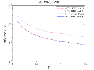
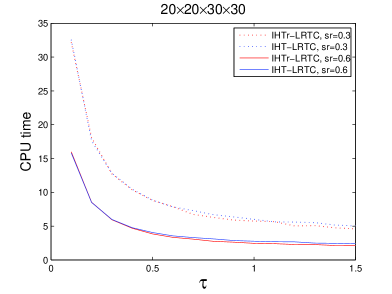
Figure 1: Recovery results with different values of $\tau$ by testing IHTr-LRTC and IHT-LRTC on random noiseless low $n$-rank tensor completion problems with the tensor of size $20\times 20\times 30\times 30$ and $n$-rank $(4,4,4,4)$. (a) relative error; (b) CPU time in seconds. All the results are average values of 10 independent trials.

Then, we compare IHTr-LRTC with IHT-LRTC on random noiseless low $n$-rank tensor completion problems with the tensor of size $50\times 50\times 50$ and $n$-rank $(9,9,3)$. The sampling ratio is set to 0.3 and 0.6, respectively. We plot the logarithm of the relative error between the $\mathcal{X}^{k}$ and the true tensor $\mathcal{M}$ versus the iteration number for algorithms IHTr-LRTC and IHT-LRTC in FIG.2 for each problem setting. From this figure, we can see that IHT-LRTC decreases $\|\mathcal{X}^{k}-\mathcal{M}\|_{F}/\|\mathcal{M}\|_{F}$ slower than IHTr-LRTC due to the heuristic of determining $r$. Additionally, for IHTr-LRTC, log$\|\mathcal{X}^{k}-\mathcal{M}\|_{F}/\|\mathcal{M}\|_{F}$ is approximately a linear function of the iteration number $k$; for IHT-LRTC, it also approximately a linear function after several iterations. This implies that the theoretical results in Theorem 4.4 approximately hold in practice.

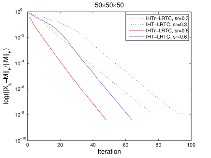
Figure 2: Relative error versus the iteration number for algorithms IHTr-LRTC and IHT-LRTC on random noiseless low $n$-rank tensor completion problems with the tensor of size $50\times 50\times 50$ and $n$-rank $(9,9,3)$. The sampling ratio is set to 0.3 and 0.6, respectively.

Table 1. Comparisons of different algorithms on random noiseless low $n$-rank tensor completion problems.
problem setting	algorithm	iter	rel.err	time(s)	problem setting	algorithm	iter	rel.err	time(s)
	IHTr-LRTC	30	7.90e-9	0.12		IHTr-LRTC	82	2.33e-8	2.32
	IHT-LRTC	41	6.52e-9	0.17		IHT-LRTC	93	2.38e-8	2.99
$\mathbb{T}=\mathbb{R}^{20\times 30\times 40}$	FP-LRTC	105	1.92e-8	0.51	$\mathbb{T}=\mathbb{R}^{60\times 60\times 60}$	FP-LRTC	520	2.00e-8	21.61
${\bm{r}}=(2,2,2)$	TENSOR-HC	66	2.09e-8	1.37	${\bm{r}}=(9,9,6)$	TENSOR-HC	49	7.23e-8	7.95
$sr=0.6$	ADM-TR(E)	216	1.02e-8	10.40	$sr=0.3$	ADM-TR(E)	410	2.37e-7	112.10
	HoRPCA	60	1.12e-8	1.53		HoRPCA	127	1.86e-8	18.09
	N-way-E	31	1.40e-8	0.91		N-way-E	68	5.61e-8	8.25
	N-way-IE	427	8.33e-2	14.38		N-way-IE	772	2.54e-2	102.57
	IHTr-LRTC	31	7.62e-9	0.92		IHTr-LRTC	90	2.23e-8	4.90
	IHT-LRTC	38	7.20e-9	1.26		IHT-LRTC	96	2.46e-8	5.28
$\mathbb{T}=\mathbb{R}^{60\times 60\times 60}$	FP-LRTC	105	6.80e-9	4.49	$\mathbb{T}=\mathbb{R}^{20\times 20\times 30\times 30}$	FP-LRTC	520	3.67e-8	135.17
${\bm{r}}=(9,9,6)$	TENSOR-HC	35	3.33e-8	5.61	${\bm{r}}=(4,4,4,4)$	TENSOR-HC	50	3.42e-7	17.13
$sr=0.6$	ADM-TR(E)	206	1.08e-8	60.62	$sr=0.3$	ADM-TR(E)	456	2.56e-7	181.87
	HoRPCA	57	1.06e-8	8.22		HoRPCA	143	2.29e-8	34.11
	N-way-E	26	9.97e-9	3.15		N-way-E	62	4.25e-8	27.75
	N-way-IE	424	2.24e-2	55.42		N-way-IE	804	3.63e-2	380.94
	IHTr-LRTC	37	9.62e-9	2.16		IHTr-LRTC	37	9.03e-9	21.55
	IHT-LRTC	45	8.10e-9	2.71		IHT-LRTC	41	1.02e-8	24.40
$\mathbb{T}=\mathbb{R}^{20\times 20\times 30\times 30}$	FP-LRTC	210	5.89e-9	16.69	$\mathbb{T}=\mathbb{R}^{20\times 20\times 20\times 20\times 20}$	FP-LRTC	135	7.18e-9	103.83
${\bm{r}}=(4,4,4,4)$	TENSOR-HC	36	3.74e-8	12.32	${\bm{r}}=(2,2,2,2,2)$	TENSOR-HC	43	4.84e-8	198.59
$sr=0.6$	ADM-TR(E)	219	1.88e-8	91.97	$sr=0.5$	ADM-TR(E)	228	4.40e-8	728.66
	HoRPCA	65	1.38e-8	15.84		HoRPCA	64	1.30e-8	207.10
	N-way-E	24	7.11e-9	11.09		N-way-E	29	5.30e-9	98.81
	N-way-IE	442	2.12e-2	207.52		N-way-IE	514	1.56e-2	1834.62

Table 1 presents the different settings for random noiseless low $n$-rank tensor completion problems and the recovery performance of different algorithms. The order of the tensors varies from three to five, and we also vary the $n$-rank and the sampling ratio $sr$. For each problem setting, we solve 10 randomly created tensor completion problems. iter, rel.err and time(s) stands for the average iterations, the average relative error and the average time (seconds) for each problem setting, respectively. From the results in Table 1, we can easily see that it costs less time with lower $n$-rank and higher sampling ratio $sr$. By comparing the results of different algorithms, it is easy to see that IHTr-LRTC and IHT-LRTC always perform better than other algorithms in both relative error and CPU time. Note that though IHT-LRTC converges a little slower than IHTr-LRTC since it needs more iterations and time to determine $n$-rank, the recoverability of IHT-LRTC can be comparable with that of IHTr-LRTC, which indicates the efficiency of the heuristic for determining $n$-rank. For the problem with relative large size (e.g., $\mathbb{T}=\mathbb{R}^{20\times 20\times 20\times 20\times 20}$, $\bm{r}=(2,2,2,2,2)$, $sr=0.5$), we can see that IHTr-LRTC and IHT-LRTC can save much more time to recover a tensor. Additionally, it’s worth noting that N-way-E also has a good performance for all the problem settings, but N-way-IE performs poorly for these problems though we just use a little higher $n$-rank. This situation indicates that the N-way toolbox depends strongly on the knowledge of the $n$-rank and the tensor may no longer be recovered with the inexact $n$-rank.

Then, we test the first seven different algorithms (N-way-IE is poorer than other algorithms obviously by Table 1) on random noiseless low $n$-rank tensor completion problems with the tensor of fixed size $100\times 100\times 100$ and different $n$-ranks $(r,r,r)$ (here we set $r_{1}=r_{2}=r_{3}=r$ for convenience). FIG.3 depict the average results of 10 independent trials corresponding to different $n$-rank $(r,r,r)$ for randomly created noiseless tensor completion problems. The sampling ratios is set to $0.5$. As indicated in FIG.3, IHTr-LRTC and IHT-LRTC are always faster and more robust than others, and provide the solutions with lower relative error.

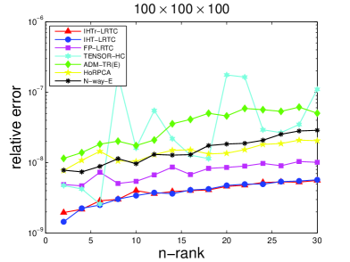
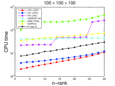
Figure 3: Recovery results by IHTr-LRTC, IHT-LRTC, FP-LRTC, TENSOR-HC, ADM-TR(E), HoRPCA and N-way-E on random noiseless low $n$-rank tensor completion problems with the tensor of fixed size $100\times 100\times 100$ and different $n$-ranks. (a) relative error; (b) CPU time in seconds. All the results are average values of 10 independent trials.

We further test the algorithms on random noisy low $n$-rank tensor completion problems. Table 2 presents the numerical performance. In the table, we report the mean of NRMSEs, iterations and execution times over 10 independent trials. Then, we set the noise level $\sigma=0.02$. From the results, we can easily see that IHTr-LRTC and IHT-LRTC are comparable with other algorithms in terms of NRMSE and CPU time.

Table 2. Comparisons of different algorithms on random noisy low $n$-rank tensor completion problems.
problem setting	algorithm	iter	NRMSE	time(s)	problem setting	algorithm	iter	NRMSE	time(s)
	IHTr-LRTC	31	2.16e-3	0.44		IHTr-LRTC	74	2.77e-3	7.70
	IHT-LRTC	38	3.71e-3	0.55		IHT-LRTC	102	3.06e-3	10.64
$\mathbb{T}=\mathbb{R}^{20\times 30\times 40}$	FP-LRTC	105	5.33e-3	1.06	$\mathbb{T}=\mathbb{R}^{60\times 60\times 60}$	FP-LRTC	520	1.19e-2	23.59
${\bm{r}}=(2,2,2)$	TENSOR-HC	45	9.22e-3	0.93	${\bm{r}}=(9,9,6)$	TENSOR-HC	31	8.88e-3	5.02
$sr=0.6$	ADM-TR(E)	142	5.24e-3	9.30	$sr=0.3$	ADM-TR(E)	301	1.20e-2	105.56
$\sigma=0.02$	HoRPCA	38	5.63e-3	0.97	$\sigma=0.02$	HoRPCA	82	1.19e-2	12.05
	N-way-E	32	1.24e-3	0.89		N-way-E	69	1.70e-3	8.23
	N-way-IE	682	3.81e-3	19.29		N-way-IE	748	2.03e-3	88.88
	IHTr-LRTC	30	2.89e-3	3.11		IHTr-LRTC	78	2.04e-3	13.50
	IHT-LRTC	39	3.22e-3	4.14		IHT-LRTC	100	2.00e-3	17.35
$\mathbb{T}=\mathbb{R}^{60\times 60\times 60}$	FP-LRTC	105	7.26e-3	5.00	$\mathbb{T}=\mathbb{R}^{20\times 20\times 30\times 30}$	FP-LRTC	520	1.45e-2	40.37
${\bm{r}}=(9,9,6)$	TENSOR-HC	23	9.64e-3	3.79	${\bm{r}}=(4,4,4,4)$	TENSOR-HC	26	9.74e-3	8.84
$sr=0.6$	ADM-TR(E)	125	6.82e-3	46.05	$sr=0.3$	ADM-TR(E)	530	1.47e-2	186.29
$\sigma=0.02$	HoRPCA	32	6.81e-2	4.69	$\sigma=0.02$	HoRPCA	355	1.46e-2	87.08
	N-way-E	26	1.34e-3	3.11		N-way-E	60	8.06e-4	26.04
	N-way-IE	444	1.49e-3	51.43		N-way-IE	925	1.21e-3	417.96
	IHTr-LRTC	35	2.68e-3	6.29		IHTr-LRTC	34	1.52e-3	83.79
	IHT-LRTC	42	2.26e-3	7.54		IHT-LRTC	45	1.21e-3	111.25
$\mathbb{T}=\mathbb{R}^{20\times 20\times 30\times 30}$	FP-LRTC	210	8.31e-3	17.46	$\mathbb{T}=\mathbb{R}^{20\times 20\times 20\times 20\times 20}$	FP-LRTC	135	6.06e-3	117.55
${\bm{r}}=(4,4,4,4)$	TENSOR-HC	21	9.81e-3	7.04	${\bm{r}}=(2,2,2,2,2)$	TENSOR-HC	15	8.50e-3	73.24
$sr=0.6$	ADM-TR(E)	204	8.01e-3	75.99	$sr=0.5$	ADM-TR(E)	422	5.76e-3	1278.79
$\sigma=0.02$	HoRPCA	128	7.98e-3	32.32	$\sigma=0.02$	HoRPCA	662	5.99e-3	2214.99
	N-way-E	24	5.80e-4	11.17		N-way-E	28	1.20e-4	95.27
	N-way-IE	450	9.20e-4	206.41		N-way-IE	441	2.32e-4	1520.44

Inpainting of color Images via low $n$-rank tensor completion. Next, we further evaluate the performance of IHTr-LRTC and IHT-LRTC on image inpainting (Bertalmío et al., 2000). Color images can be expressed as third-order tensors. If the image is of low $n$-rank, or numerical low $n$-rank, we can solve the image inpainting problem as a low $n$-rank tensor recovery problem. In our test, we first compute the best rank-$(r_{1},r_{2},r_{3})$ approximation of a color image to obtain an numerical low $n$-rank image. Then, we randomly remove the values of some of the pixels of the numerical low $n$-rank image, and want to fill in these missing values.

Remark: The best rank-$(r_{1},r_{2},\cdots,r_{N})$ approximation is used as a tool for dimensionality reduction and signal subspace estimation. Several algorithms for this purpose have been proposed in the literature, e.g., the higher-order orthogonal iteration (HOOI) (Lathauwer et al., 2000). More details can be seen in Ishteva (2009). Note that the N-way toolbox for Matlab is also an effective and convenient tool of computing the best rank-$(r_{1},r_{2},\cdots,r_{N})$ approximation. However, considering to be fair and reasonable, we here use the MATLAB Tensor Toolbox by Bader et al. (2012), which is an another famous tool for tensor computation, to compute the best rank-$(r_{1},r_{2},\cdots,r_{N})$ approximation. Using Matlab notation, for a tensor $\mathcal{X}\in\mathbb{R}^{n_{1}\times n_{2}\times\cdots\times n_{N}}$, $\bar{\mathcal{X}}=\mathrm{tucker}\_\mathrm{als}(\mathcal{X},[r_{1}~{}r_{2}\cdots r_{N}])$ returns the best rank-$(r_{1},r_{2},\cdots,r_{N})$ approximation of $\mathcal{X}$. Additionally, the parameter $\xi$ in predicting $n$-rank is set to $10^{-4}$ to guarantee the better prediction of $n$-rank for the practical problems.

FIG.4 and FIG.5 respectively present the recovered images for the best rank-$(30,30,3)$ and rank-$(100,100,3)$ approximation of the original $512\times 512$ image by different algorithms (Here, ADM-TR(E) and N-way-IE perform poorer than others obviously, so their results are no longer reported). The sampling ratio is set to 0.3. We also report the numerical results in Table 3. Although the recovered images of these five algorithms are similar visually to each other, the results in Table 3 show that IHTr-LRTC and IHT-LRTC are more effective than others, especially for the problem with high $n$-rank. More specifically, for the best rank-$(30,30,3)$ approximation of the original image, all the algorithms can recover the image well by using only 30% of pixels and IHTr-LRTC is much faster than others. For the best rank-$(100,100,3)$ approximation of the original image, we can see that the relative errors of recovered images by FP-LRTC, TENSOR-HC and HoRPCA are very large due to the relatively high $n$-rank. However, IHTr-LRTC and IHT-LRTC can also perform well.

Figure 4: Comparisons of different algorithms for image inpaiting. The right two columns are recovery results of different algorithms. Specifically, (a) Original $512\times 512$ image; (d) The best rank-$(30,30,3)$ approximation of original image; (g) Input to the algorithm (30% known entries); (b) Recovered image by IHTr-LRTC; (e) Recovered image by IHT-LRTC; (h) Recovered image by FP-LRTC; (c) Recovered image by TENSOR-HC; (f) Recovered image by HoRPCA; (i) Recovered image by N-way-E.

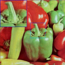
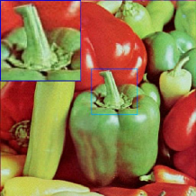
Figure 5: Comparisons of different algorithms for image inpaiting. The right two columns are recovery results of different algorithms. Specifically, (a) Original $512\times 512$ image; (d) The best rank-$(100,100,3)$ approximation of original image; (g) Input to the algorithm (30% known entries); (b) Recovered image by IHTr-LRTC; (e) Recovered image by IHT-LRTC; (h) Recovered image by FP-LRTC; (c) Recovered image by TENSOR-HC; (f) Recovered image by HoRPCA; (i) Recovered image by N-way-E.

Table 3. Numerical results of different algorithms for image inpainting
Algorithm	iter	rel.err	time(s)	Algorithm	iter	rel.err	time(s)
$size=512\times 512\times 3$, $sr=0.3$
${\bm{r}}=(30,30,3)$				${\bm{r}}=(100,100,3)$
IHTr-LRTC	187	1.06e-7	32.46	IHTr-LRTC	1733	5.02e-7	332.05
IHT-LRTC	665	6.40e-8	128.68	IHT-LRTC	5000	7.24e-4	998.69
FP-LRTC	1040	5.17e-7	454.13	FP-LRTC	1040	5.40e-2	629.40
TENSOR-HC	144	1.81e-7	246.65	TENSOR-HC	775	4.58e-2	1337.67
HoRPCA	138	3.33e-7	93.69	HoRPCA	1000	4.55e-2	1198.55
N-way-E	107	4.72e-7	121.64	N-way-E	618	1.34e-4	1336.11

7 Conclusions

In this paper, we considered a new alternative recovery model ‘MnRA’ and proposed an appropriate iterative hard thresholding algorithm to solve it with giving upper bound of $n$-rank in advance. The convergence analysis of the proposed algorithm was also presented. By using an effective heuristic of determining $n$-rank, we can also apply the proposed algorithm to solve MnRA with unknown $n$-rank in advance. Some preliminary numerical results on LRTC were reported. Through the theoretical analysis and numerical experiments, we can draw some encouraging conclusions:

• The model of MnRA in this paper is creative in low $n$-rank tensor recovery. MnRA includes both noiseless and noisy case. And although the model needs the $n$-rank of the original data as prior information, we have proposed a heuristic for determining $n$-rank and this method turned to be efficient.

• The iterative hard thresholding algorithm proposed in this paper is easy to implement. It has a very simple iterative scheme and only one parameter $\tau$, which can be easily estimated from theoretical analysis and can be chosen broadly in practice.

• The iterative hard thresholding algorithm is extremely fast. Actually, the iterative sequence generated by the proposed algorithm is globally linearly convergent with the rate $\frac{1}{2}$ for the noiseless case. In our numerical experiments, these theoretical results can be confirmed.

• IHTr-LRTC and IHT-LRTC are still effective for the tensor with high $n$-rank. Thus, they may have wider applications in practice.

It is interesting to investigate how to determine $n$-rank more effectively in practice. We believe that the iterative hard thresholding algorithm combining with the appropriate method for predicting $n$-rank can be used to solve more general tensor optimization problems. Moreover, the nonconvex sparse optimization problems and the related algorithms in vector or matrix space have been widely discussed in the literature (Zhang et al., 2013; Li et al., 2014). It is worth investigating how to apply the iterative hard thresholding algorithm to solve the nonconvex model in the tensor space.

References

- Andersson & Bro (2000) Andersson, C.A. & Bro, R.(2000) The N-way Toolbox for MATLAB Chemometrics & Intelligent Laboratory Systems, 52, 1–4, http://www.models.life.ku.dk/source/nwaytoolbox/
- Argyriou et al. (2008) Argyriou, A., Evgeniou, T. & Pontil, M. (2008) Convex multi-task feature learning Mach. Learn., 73, 243–272
- Bader et al. (2012) Bader, B. W., Kolda, T. G. & others (2012) MATLAB Tensor Toolbox Version 2.5. Available online URL: http://www.sandia.gov/ tgkolda/TensorToolbox/
- Bertalmío et al. (2000) Bertalmío, M., Sapiro, G., Caselles, V. & Ballester, C. (2000) Image inpainting Proceedings of SIGGRAPH 2000, New Orleans, USA
- Blumensath & Davies (2008) Blumensath, T. & Davies, M. E. (2008) Iterative thresholding for sparse approximations J. Fourier Anal. Appl., 14, 629–654
- Blumensath & Davies (2009) Blumensath, T. & Davies, M. E. (2009) Iterative hard thresholding for compressed sensing Appl. Comput. Harmon. Anal., 27, 265–274
- Blumensath (2012) Blumensath, T. (2012) Accelerated iterative hard thresholding Signal Process., 92, 752–756
- Blumensath et al. (2012) Blumensath, T., Davies, M. E. & Rilling, G. (2012) Compressed Sensing: Theory and Applications Cambridge University Press
- Biswas et al. (2006) Biswas, P., Lian, T. C., Wang, T. C. & Ye Y. (2006) Semidefinite programming based algorithms for sensor network localization ACM Trans. Sensor Network., 2, 188–220
- Bresler & Lee (2009) Bresler, Y. & Lee, K. (2009) Efficient and guaranteed rank minimization by atomic decomposition Information Theory, ISIT 2009, IEEE International Symposium on., 314-318
- Candès & Recht (2009) Candès, E. J. & Recht, B. (2009) Exact matrix completion via convex optimization Found. Comput. Math., 9, 717–772
- Dai et al. & Kerman (2011) Dai, W., Milenkovic, O. & Kerman, E. (2011) Subspace evolution and transfer (SET) for low-rank matrix completion IEEE Trans. Signal Process., 59, 3120–3132
- Dai & Milenkovic (2009) Dai, W. & Milenkovic, O. (2009) Subspace pursuit for compressive sensing signal reconstruction IEEE Trans. Inform. Theory, 55, 2230–2249
- Drineas et al. (2006) Drineas, P., Kannan, R. & Mahoney, M. W. (2006) Fast monte carlo algorithms for matrices II: computing low-rank approximations to a matrix SIAM J. Comput., 36, 158–183
- Gandy et al. (2011) Gandy, S., Recht, B. & Yamada, I. (2011) Tensor completion and low--rank tensor recovery via convex optimization Inv. Probl., 27, 025010
- Goldberg et al. (1992) Goldberg, D., Nichols, D., Oki, B. M. & Terry, D. (1992) Using collaborative filtering to weave an information tapestry. Commun. ACM, 35, 61–70.
- Goldfarb & Ma (2011) Goldfarb, D. & Ma, S. (2011) Convergence of fixed point continuation algorithms for matrix rank minimization Found. Comput. Math., 11, 183–210
- Goldfarb & Qin (2014) Goldfarb, D. & Qin, Z.W. (2014) Robust low-rank tensor recovery: Models and algorithms SIAM J. Matrix Anal. Appl., 35, 225–253
- Haldar & Hernando (2009) Haldar, J. & Hernando, D. (2009) Rank-constrained solutions to linear matrix equations using power factorization IEEE Signal Process. Lett., 16, 584–587
- Ishteva (2009) Ishteva, M. (2009) Numerical methods for the best low multilinear rank approximation of higher-order tensors Ph. D. thesis, Department of Electrical Engineering, Katholieke Universiteit Leuven
- Keshavan et al. (2010) Keshavan, R., Montanari, A. & Oh, S. (2010) Matrix completion from a few entries IEEE Trans. Inform. Theory, 56, 2980–2998
- Keshavan & Oh (2009) Keshavan, R. H. & Oh, S. A. (2009) Gradient descent algorithm on the grassman manifold for matrix completion arXiv:0910.5260
- Kolda & Bader (2009) Kolda, T. G. & Bader, B. W. (2009) Tensor decompositions and applications SIAM Rev., 51, 455–500
- Kyrillidis & Cevher (2014) Kyrillidis, A. & Cevher, V. (2014) Matrix recipes for hard thresholding methods J. Math. Imaging Vis., 48, 235–265
- Larsen (2004) Larsen, R. M. (2004) PROPACK-software for large and sparse svd calculations available at http://sun.stanford. edu/srmunk/PROPACK/
- Lathauwer et al. (2000) Lathauwer, L. De., Moor, B. De. & Vandewalle, J. (2000) On the best rank-1 and rank- approximation of higher-order tensors SIAM J. Matrix Anal. Appl., 21, 1324–1342
- Lee & Bresler (2010) Lee, K. & Bresler, Y. (2010) Admira: Atomic decomposition for minimum rank approximation IEEE Trans. Inform. Theory, 56, 4402–4416
- Liu et al. (2009) Liu, J., Musialski, P., Wonka, P. & Ye, J. P. (2009) Tensor completion for estimating missing values in visual data IEEE Int. Conf. Computer Vision (ICCV), 2114–2121
- Liu & Vandenberghe (2009) Liu, Z. & Vandenberghe, L. (2009) Interior-point method for nuclear norm approximation with application to system identification SIAM J. Matrix Anal. Appl., 31, 1235–1256
- Li et al. (2014) Li, Y. F., Zhang, Y. J. & Huang, Z. H. (2014) A reweighted nuclear norm minimization algorithm for low rank matrix recovery J. Comput. Appl. Math., 263, 338–350
- Ma et al. (2011) Ma, S. Q., Goldfarb, D. & Chen, L. F. (2011) Fixed point and Bregman iterative methods for matrix rank minimization Math. Program., 128, 321–353
- Needell & Tropp (2008) Needell, D. & Tropp, J. A. (2008) CoSaMP: iterative signal recovery from incomplete and inaccurate samples Appl. Comput. Harmon. Anal., 26, 301–321
- Portilla (2009) Portilla, J. (2009) Image restoration through analysis-based sparse optimization in tight frames In Image Processing (ICIP), 2009 16th IEEE International Conference on IEEE., 3909–3912
- Recht et al. (2010) Recht, B., Fazel, M. & Parrilo, P. A. (2010) Guaranteed minimum-rank solutions of linear matrix equations via nuclear norm minimization SIAM Rev., 52, 471–501
- Shi et al. (2013) Shi, Z. Q., Han, J. Q., Zheng, T. R. & Li, J.(2013) Guarantees of augmented trace norm models in tensor recovery Proceedings of the Twenty-Third international joint conference on Artificial Intelligence, AAAI Press, 1670–1676
- Signoretto et al. (2010) Signoretto, M., Lathauwer, L. De. & Suykens, J. A. K. (2010) Nuclear norms for tensors and their use for convex multilinear estimation Internal report 10-186, ESAT-SISTA, K.U. Leuven, Leuven, Belgium. Lirias number: 270741
- Signoretto et al. (2013) Signoretto, M., Tran, Dinh. Q., Lathauwer, L. De. & Suykens, J. A. K. (2013) Learning with tensors: a framework based on convex optimization and spectral regularization Mach. Learn., 94, 303–351
- Yang et al. (2013) Yang, L., Huang, Z. H. & Shi, X. J. (2013) A fixed point iterative method for low n-rank tensor pursuit IEEE Trans. Signal Process., 61, 2952–2962
- Yang et al. (2013) Yang, L., Huang, Z. H., Hu, S. L. & Han, J. Y. (2013) An iterative algorithm for third-order tensor multi-rank minimization Comput. Optim. Appl. revised
- Zhang & Huang (2012) Zhang, M. & Huang, Z. H. (2012) Exact recovery conditions for the low--rank tensor recovery problem via its convex relaxation preprint.
- Zhang et al. (2013) Zhang, M., Huang, Z. H. & Zhang, Y.(2013) Restricted -isometry properties of nonconvex matrix recovery IEEE Trans. Inform. Theory, 59, 4316–4323