The Link Between Ejected Stars, Hardening and Eccentricity Growth of Super Massive Black Holes in Galactic Nuclei

Abstract

The hierarchical galaxy formation picture suggests that super massive black holes (MBHs) observed in galactic nuclei today have grown from coalescence of massive black hole binaries (MBHB) after galaxy merging. Once the components of a MBHB become gravitationally bound, strong three-body encounters between the MBHB and stars dominate its evolution in a “dry” gas free environment, and change the MBHB’s energy and angular momentum (semi-major axis, eccentricity and orientation). Here we present high accuracy direct $N$-body simulations of spherical and axisymmetric (rotating) galactic nuclei with order $10^{6}$ stars and two massive black holes that are initially unbound. We analyze the properties of the ejected stars due to slingshot effects from three-body encounters with the MBHB in detail. Previous studies have investigated the eccentricity and energy changes of MBHs using approximate models or Monte-Carlo three body scatterings. We find general agreement with the average results of previous semi-analytic models for spherical galactic nuclei, but our results show a large statistical variation. Our new results show many more phase space details of how the process works, and also show the influence of stellar system rotation on the process. We detect that the angle between the orbital plane of the MBHBs and that of the stellar system (when it rotates) influences the phase-space properties of the ejected stars. We also find that massive MBHB tend to switch stars with counter-rotating orbits into co-rotating orbits during their interactions.

1 Introduction

The current galaxy formation scenario based on the $\Lambda$ cold dark matter ($\Lambda$CDM) cosmology model (Begelman et al., 1980; Volonteri et al., 2003) suggests that massive galaxies form from hierarchical merging and accretion of smaller galaxies. If the merging galaxies have massive black holes (MBHs) in their centers, the merging processes should also include coalescence of MBHs, since MBHs are commonly observed at the centers of most galaxies today (Greene & Ho, 2009). Thus, to understand the process of MBHs coalescence is significant for cosmological structure formation, galaxy formation and MBH formation.

In the case of gas-poor galaxies merging, the two MBHs have three distinct evolution phases (Begelman et al., 1980). First, the dynamical friction exerted by the stars forces the two MBHs to sink toward the galactic center. This phase continues until the binary reaches the hard binary separation (Merritt, 2001; Yu, 2002). Second, a hard MBH binary (MBHB) orbit will continue to shrink due to slingshot ejection of surrounding stars. Third, when the MBHB reaches a separation at which the loss of orbital energy caused by gravitational waves (GWs) emission becomes significant, the MBHB shrinks until the final coalescence.

There is a challenging problem, often called “Final Parsec Problem”, during this three phase model in the merger of gas-poor galaxies. In quasi-steady spherical stellar environment, the slingshot efficiency decreases rapidly when the separation of the MBHB becomes much smaller than the average separation of neighboring stars of the MBHB (Quinlan & Hernquist, 1997; Milosavljević & Merritt, 2003; Berczik et al., 2005). The hardening rate of the MBHB for large particle numbers, such as in real galactic nuclei, is too low and the timescale of coalescence of the MBHB will be larger than the Hubble time. Recent efforts suggest that if the stellar system has some degree of axisymmetry or triaxiality, this problem may be solved (Yu, 2002; Merritt & Poon, 2004; Berczik et al., 2006; Preto et al., 2011; Fiestas et al., 2012; Khan et al., 2012b, 2013). The simulations by Khan et al. (2013) show that even a mildly flattened stellar system with an axis ratio of $0.9$ will result in an eight times faster hardening rate of the MBHB, and that the MBHB evolution is independent of particle number when the axis ratio is $0.75$. These results agree with the earlier work of Berczik et al. (2006). Also, Gualandris & Merritt (2012) argue that in post-merger galaxies the loss-cone is full, hardening does not depend on $N$. Therefore, these studies show a solution of the “Final Parsec Problem” because the MBHB merges in a relatively short time. The final solution of this problem requires more work on the details of the slingshot phase.

Detection of GWs is the most important expected observations in the near future to give direct proof of general relativity. GWs will also provide a new window to understand the Universe independent of electromagnetic observations. The coalescence of MBHs is expected to be the strongest GW source to be measured with future space satellite detectors, such as the Laser Interferometer Space Antennae (LISA/e-LISA/ALIA, see e.g. Gong et al., 2011). This encourages researchers to concentrate on the final orbital parameters and the merging rate of MBHs to predict the GW signals to be measured.

It is very important to understand the eccentricity growth of the MBHB during phase $2$ since it strongly influences the coalescence time (Peters, 1964) and the angular momentum evolution. Quinlan (1996) used three-body scattering experiments to study the properties of slingshot effects. He found the eccentricity growth is small unless the MBHB already forms with a large eccentricity. Preto et al. (2011); Khan et al. (2011) carried out a large number of $N$-body simulations of equal-mass MBHBs in axisymmetric and triaxial stellar environment after a galaxy merger. They found the initial eccentricities when MBHs become bound are very high with about $e=0.95$ on average. This is also consistent with previous work (Aarseth, 2003; Berentzen et al., 2008, 2009a; Preto et al., 2009; Li et al., 2012). On the other hand, Khan et al. (2013) find low eccentricities for some of their elliptical galaxy models. The reason for this may be that they model a non-rotating stellar system. However, none of the these studies examined the detailed scattering processes near the MBHB; it is desirable to study the eccentricity evolution in detail in the full $N$-body simulation as a counterpart, and to check the validity of Quinlan (1996) three-body Monte Carlo work.

A galaxy merger can result in a rotating stellar system. Therefore, simulations of MBHBs in rotating star clusters are interesting (Berczik et al., 2006; Preto et al., 2011; Khan et al., 2011, 2012b). Several restricted studies of MBHB evolution in rotating star clusters were carried out by Sesana et al. (2011) and Gualandris et al. (2012). They study very high mass ratios of the MBHB ($1/64$) and a small stellar system surrounding it (less than the mass of the MBHB). Under these restrictions, Sesana et al. (2011) find that the eccentricity evolution of MBHB in a rotating stellar cusp can be significantly influenced by the fraction of corotating stars. However, larger $N$-body simulations may give different results, because many interactions occur with stars from unbound regious. Thus to understand the effect of stellar rotation further, it is necessary to carry out a deeper analysis of large $N$-body systems with different mass ratios of MBHB.

It is interesting that triple black holes during galaxy mergers can also exist, if one of the progenitor MBHBs does not coalesce before the next galaxy with another third MBH falls in. In such cases, very extreme eccentricities of the inner MBHB have been found ($e\sim 0.99-0.999$, Amaro-Seoane et al., 2010)

Yu & Tremaine (2003) studied the dynamical processes of hyper-velocity stars ejected by the MBHB in the Galactic center and predicted the rate of ejections. Lu et al. (2010) use analytical arguments and numerical simulations to study the distribution of hyper-velocity stars ejected by a MBH in the Galactic center. They found most of these are ejected anti-parallel to the injecting direction of their progenitors.

In this paper, Section 2 provides the $N$-body simulations and the method to select ejected stars from the simulation results. In Section 3 we list the initial conditions. In Section 4 we discuss the eccentricity growth of MBHBs, angular momentum properties of MBHBs and ejected stars. Finally, Section 5 contains our results and conclusions.

2 Methods

In this work, we use the direct $N$-body code called $\varphi$GPU  (Berczik et al., 2011) to do all the simulations. The full set of runs and the parameters are described in more detail in our forthcoming publication  (Berczik et al., 2013a).

The code is a direct $N$-body simulation package, with a high order Hermite integration scheme and individual block time steps (the code supports time integration of particle orbits with 4^th, 6^th and even 8^th order schemes). A direct $N$-body code evaluates in principle all pairwise forces between the gravitating particles, and its computational complexity scales asymptotically with $N^{2}$; however, it is not to be confused with a simple brute force shared time step code, due to the block time steps. We refer more interested readers to a general discussion about $N$-body codes and their implementation in Spurzem et al. (2011a, b).

The $\varphi$GPU code is fully parallelized using the MPI library, and for each MPI process GPU accelerator hardware is used to compute gravitational forces between particles. It is based on an earlier C version for GRAPE6a clusters  (Fukushige et al., 2005). The new code is written from scratch in C++ and based on earlier CPU serial $N$-body code (YEBISU; Nitadori & Makino, 2008 ). The MPI parallelization was done in the same “j” particle parallelization mode as in the earlier $\varphi$GRAPE code (Harfst et al., 2007).

The present version of the $\varphi$GPU code uses native GPU support and direct access to the GPU’s with only the NVIDIA native CUDA library. Multi GPU support is achieved through MPI parallelization. More details and also the $\varphi$GPU public version are presented in Berczik et al. (2011); Spurzem et al. (2012); Berczik et al. (2013b).

The present code is well tested and already used to obtain important results in our earlier large scale few million body simulation  (Khan et al., 2012a).

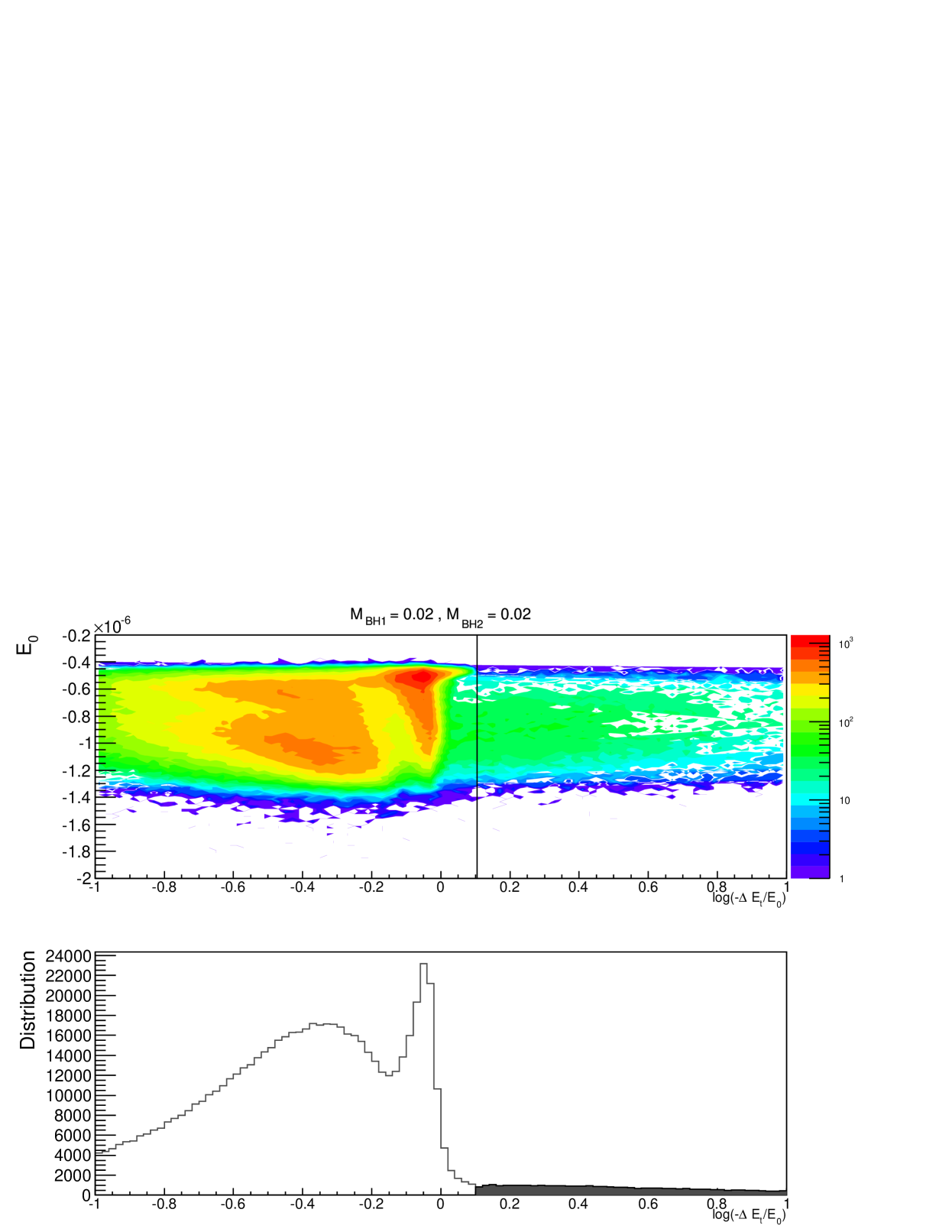
(a)

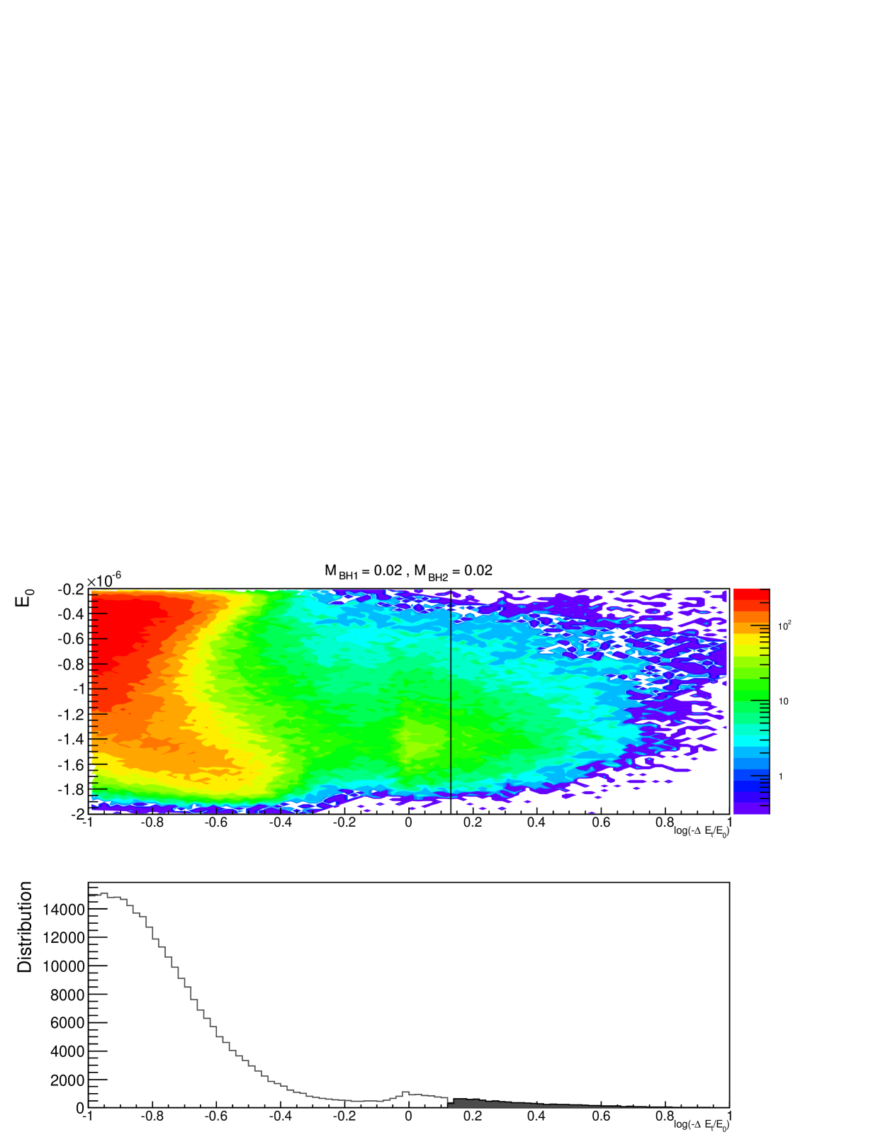
(b)

Figure 1: The total energy change of individual stars for model $2020$ (a) and $2020$-nonrot (b). the upper panels in (a) and (b) are two-dimension histograms of $E_{0}$ vs. $\log(-\Delta E_{t}/E_{0})$. The bottom panels in (a) and (b) show the distributions of $\log(-\Delta E_{t}/E_{0})$. The black line is threshold determined by the critical value $\delta_{e}$ which separates the two number density populations (Section 2). The stars in right regions are selected as ejected star candidates.

Our analysis is based on the ejected stars from the slingshot effect of MBHBs. The method used to select ejected stars depends on the individual total energy change from the beginning to the end of the simulations ($\Delta E_{t}$) because ejected stars usually gain a lot of energy during the interaction and this energy gain should be much larger than energy fluctuations caused by perturbations from other stars. The next step is to check the two dimensional histogram of initial energy of each star $E_{0}$ vs. $\log(-\Delta E_{t}/E_{0})$ for each model, and to determine a critial value $\delta_{e}$ to select ejected star candidates, which satisfy $\log(-\Delta E_{t}/E_{0})>\delta_{e}$, where $\delta_{e}$ is obtained by the number density gap shown in Figure 1. For rotating and non-rotating models, these energy features are different, but we still can select a $\delta_{e}$, which works well. This procedure also functions as an operational definition of the term ejected star, which here just means it leaves after a strong encounter with the MBHB with significantly higher energy than before. For the purpose of our paper it is not important whether the ejected star has enough energy to become unbound from the MBHB, from the central stellar cluster or even from the entire galaxy.

The next step is to check the energy evolution of each ejected star candidate and the MBHB. The final samples of stars are chosen from each candidate energy change $\Delta E_{i}>M_{s,i}$ during its ejection time $t_{e}$, where $M_{s,i}$ is the mass of a star in $N$-body units and $i$ indicates the index of ejected stars. In our simulation, $M_{s,i}$ is the same order of magnitude of the individual star’s energy in $N$-body units. Thus it can be used to select the events with obvious energy jump.

With the ejected stars samples, we calculate the angular momentum $L_{i}$ of each ES and $L_{b}$ of the MBHB at $t_{e}$. We compare the angular momentum before and after ejection of each star.

We carry out all data reduction and analysis using the open source software ROOT.

3 Units and Initial Conditions

We scale the numerical units of our initial models applying the standard $N$- body normalization (Aarseth et al., 1974) by setting both the gravitational constant $G$ and the total mass of the stellar system to unity. The total energy of the system is scaled to $E=-{1/4}$. Our simulations are purely gravitational and thus scale-free, but for convenience we define one example of the scaling in physical units below. The initial conditions of our $N$-body simulations presented here are based on the ones used in Berczik et al. (2006) and Berentzen et al. (2009b). The initial stellar galactic nucleus follows a distribution function for a rotating King model (see, e.g., Einsel & Spurzem, 1999, and references therein). It provides rigid rotation inside the half-mass radius, and quickly decreasing differential rotation outwards. After the MBHs settle into the galactic center the density and velocity dispersion adjust to the MBH’s gravity inside its influence radius. The concentration and rotation parameters are set to $W_{0}=6$ and to $\omega_{0}=1.8$, respectively, in all rotating models. We also simulate the non-rotating King models ($\omega_{0}=0$) for comparison. The total angular momentum vector of the stellar nucleus are aligned with the $z$-axis of our coordinate frame. We place the two MBHBs in the $z=0$ mid-plane with initial coordinate components $x_{1,2}=0$ and $y_{1,2}=\pm 0.3$, where the subscripts denote the two black hole particles.

The full set of models (with different field particle numbers and set of MBH’s initial velocities) and the MBH’s orbital evolution are presented elsewhere (Berczik et al., 2013a). Here we analyze only the subset of our runs (which include seven models) with a fixed stellar particle number $N=10^{6}$. The total integration time for these models was $150$ $N$-body time units. The differences are the MBH masses, which we are given in Table 1. The non-rotating models are indicated by the suffix -nonrot hereafter. Our work will focus on the rotating models. Thus non-rotating models will only be shown in some parts. The initial $x$-velocity of the MBH’s in these simulations has been chosen to be $v_{x;1,2}=\pm V_{\mathrm{circ}}$, where $V_{\mathrm{circ}}$ is the circular velocity within the stellar background model. With our choice of initial values, the circular velocity in $N$-body units is $V_{\mathrm{circ}}=0.7$ at the initial distance of the MBH’s from the center.

Our models are scale-free and can be applied to a range of real astrophysical systems. Here we give an example, for the case of the MBH mass 0.01 in $N$-body units i (see Table 1); if the black hole mass is e.g. $10^{7}M_{\odot}$, and the black hole separation $y_{1,2}=\pm 0.3$ is, e.g., $\pm 300$ pc, then one $N$-body time unit is about $15$ Myr and one $N$-body velocity unit is about $65.6$ km/s.

Table 1: Full set of our model runs for both rotating and non-rotating King models (we use $W_{0}=6$ and $\omega_{0}=1.8$ for the rotating and $\omega_{0}=0$ for the non-rotating models). $m_{1}$, $m_{2}$ and $\mu=m_{1}m_{2}/M$, with $M=m_{1}+m_{2}$ denote the masses of the primary and secondary MBH and their reduced mass; all masses here are in units of $10^{-2}$, where the total cluster mass is unity.

Model	0110	0210	0510	1010	2020	4020	4040
$m_{2}/m_{1}$	0.10/1	0.20/1	0.50/1	1.00/1	2.00/2	4.00/2	4.00/4
$\mu$	0.0909	0.1667	0.3333	0.5000	0.6667	1.3333	2.0000

4 Results

4.1 Coordinate System and Angles

In our simulations, we have initially defined rectangular, Cartesian coordinates with $x$, $y$ and $z$ axes (Section 3). Here, we define three angles: $\alpha$, $\delta$ and $\theta$. When we use the spherical coordinate system instead, the radius $r$ denotes the distance to the origin and two angles $\alpha$ and $\delta$ define the direction of a vector. The transformation from $(x,y,z)$ to $(r,\alpha,\delta)$ can be described as:

$$\begin{split}x&=r\cos\delta\cos\alpha\\ y&=r\cos\delta\sin\alpha\\ z&=r\sin\delta\\ \end{split}$$ (1)

We will later use these spherical coordinates to define the angular momentum vectors of a star $L_{s}$ and of the MBHB $L_{b}$. $\theta$ is the angle between $L_{b}$ and $L_{s}$ defined through:

$$\theta=\arccos\frac{\overrightarrow{L_{b}}\cdot\overrightarrow{L_{s}}}{|\overrightarrow{L_{b}}||\overrightarrow{L_{s}}|}$$ (2)

Hereafter we use suffix “b” to denote MBHBs and “s” to denote ejected stars.

For each angle of individual ejected stars or MBHBs, we also have two values: the one before ejection time $t_{i}$ (hereafter denoted with suffix “BE”) and the one after ejection time $t_{o}$ (hereafter denoted with suffix “AE”). Due to our simulation output time resolution, the interval time between $t_{i}$ and $t_{o}$ is one $N$-body time unit.

4.2 Ejected Stars Sample Selection

Using the method discussed in Section 2, we successfully find most ejected stars for the massive MBHB models. The numbers of ejected stars and $\delta_{e}$ (defined in Section 2) for all rotating models are listed in Table 2.

Table 2: The number of ejected stars detected in each rotating model.

Model	0110	0210	0510	1010	2020	4020	4040
$\delta_{e}$	0.25	0.25	0.24	0.20	0.24	0.19	0.08
$N_{ESs}$	863	3457	10203	16656	40288	57596	83367
$N_{ESs}/N_{tot}(\%)$	$0.086$	$0.34$	$1.02$	$1.67$	$4.03$	$5.76$	$8.34$

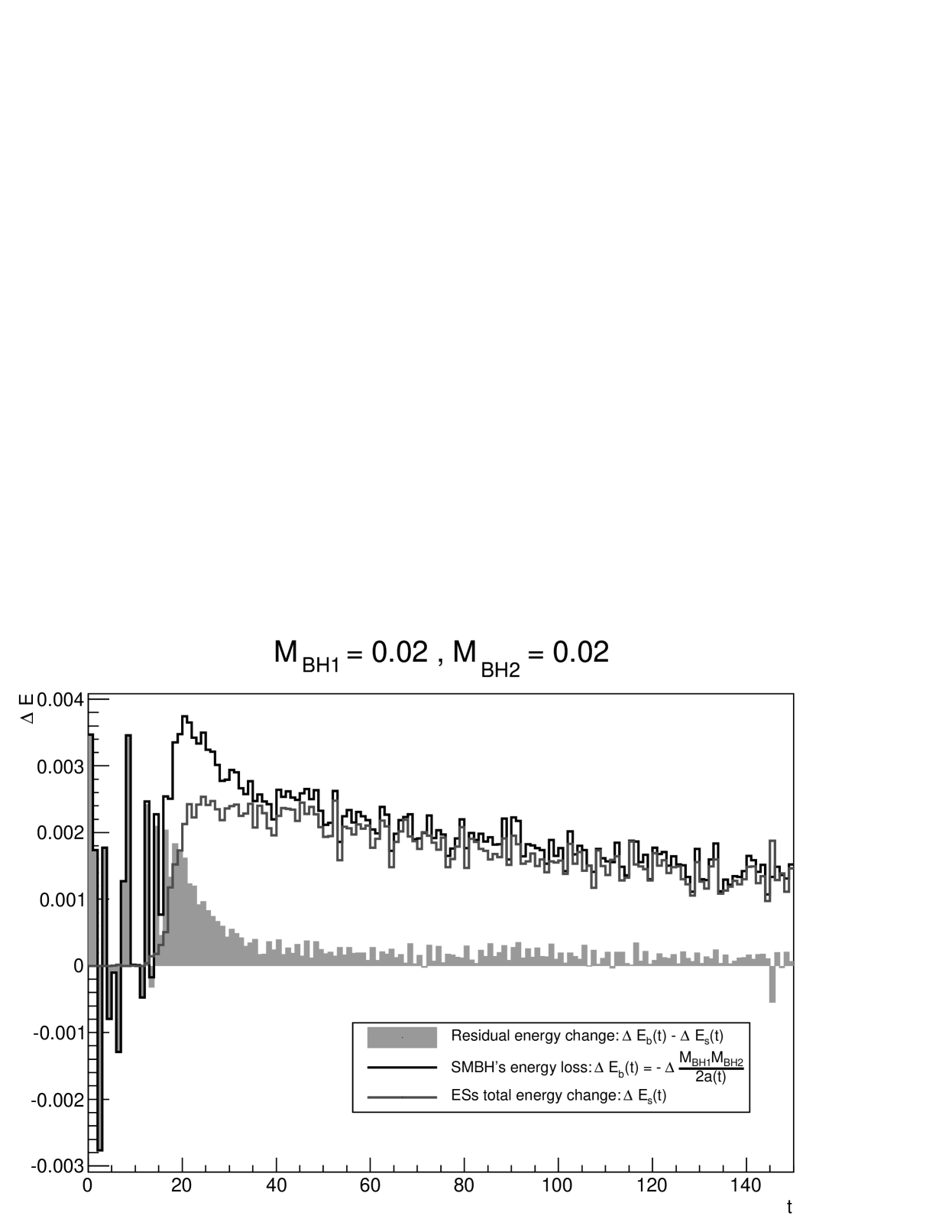
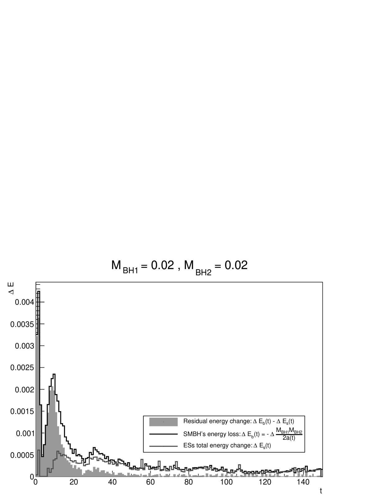
Figure 2: The histogram of energy change of MBHBs, ejected stars and residual energy with respect to time, for model $2020$ and $2020$-nonrot (see Table 1). $\Delta E_{s}(t)$ is the integration of energy change of ejected stars ejecting bewteen time $t$ and $t+1$ ($N$-body unit).

To ensure our samples are convincing, we calculate the integrated energy change of all ejected stars during their ejections ($\Delta E_{s}(t)$) and compare it to the MBHBs’ binding energy loss ($\Delta E_{b}(t)$) during each time unit (Figure 2). If the residual energy change $\Delta E_{r}(t)=\Delta E_{b}(t)-\Delta E_{s}(t)$ is zero, the ejected star sample is complete, its deviation from zero gives information about how many ejected stars we may have missed, since there is no other significant mechanism in our simulations due to which the MBHB can lose energy. Figure 2 shows that $\Delta E_{r}(t)$ in both the rotating model $2020$ and the non-rotating model $2020$-nonrot are almost zero after the binary formation ($t>40$). This result holds for all models with large black hole masses. This indicates our method to select ejected stars is reliable. The only exceptions are the two models $0110$ and $0210$ with low masses of MBHBs (one is shown in Figure 2).

There are two possibilities that may cause incomplete samples for low mass MBHBs. One is that low mass MBHBs probably generate more ejected stars with low $\Delta E_{i}$, which cannot be distinguished from energy fluctuations caused by other mechanisms, so we cannot select this part of the ejected stars. Another reason is that the low mass MBHB’s become gravitational bound at a later time than the massive ones – slingshot effects dominate the energy loss of MBHBs only after the binary formation.

4.3 Eccentricity Growth Rate of MBHBs

The specific angular momentum $J$ of a MBHB can be described by

$$J=\frac{L}{\mu}=\sqrt{GMa(1-e^{2})}$$ (3)

where $L$ is the standard angular momentum, $\mu$ is reduced mass, $a$ is semi-major axis, $M=m_{1}+m_{2}$ is the total mass of the binary components, $e$ is the eccentricity and $G$ is gravitational constant. The hardening process of a MBHB provides energy to the ejected stars, and thus increases its binding energy and reduces its semi-major axis $a$; As a result of Eq. 3 the angular momentum of the MBHB will also be reduced, even if $e$ remains constant (which is generally not the case; see below). Any eccentricity growth will lead to additional decrease of $L$. In phase $2$, the ejected stars dominate the energy and angular momentum evolution of MBHB. Thus to understand the properties of ejected stars it will help to know how they carry away the energy and the angular momentum from the MBHB.

Quinlan (1996) defined an eccentricity growth rate $K$ as

$$K=\frac{\Delta e}{\Delta\ln(1/a)}$$ (4)

and then derived $K_{1}$, a numerical expression of $K$ with the assumption that all stars have an identical velocity $v$. Note that, for the special case of constant specific angular momentum ($\Delta J=0$), we have

$$K=\frac{\Delta e}{\Delta\ln(1/a)}=-\frac{1-e^{2}}{2e}\ .$$ (5)

Quinlan also carried out Monte-Carlo models (three-body scattering experiments of single stars with the MBHB), the results of which we can compare with our data. In our work, we also calculate $K$ by using Equation 4 directly from the MBHBs measured changes $\Delta e$ and $\Delta\ln(1/a)$. To compute the differences we use the eccentricity $e$ and semi-major axis $a$ of the MBHB averaged over time spans of one $N$-body time unit (for good statistic).

Figure 3 shows the comparison between our result with Quinlan (1996)’s. The values are not monotonous in time, rather there is a stochastic variation of $K$ (which creates positive and negative $\Delta e$ in individual encounters) due to the three-body encounters. The average growth rate of $e$ (see circles with crosses in Figure 3) is positive and agrees fairly well with previous semi-analytic work. The dash-dotted line shows the predicted growth rate when $J$ of MBHB is conserved. If $J$ of MBHB decreases as the MBHB become harding, the $K$ should be located above this line. Our results indicate that during the hardening of the MBHB, the MBHBs with lower $e$ always lose $J$ and the MBHBs with higher $e$ in most cases also lose $J$.

4.4 Angular Momentum exchange between stars and MBHBs

4.4.1 Angular momentum evolution

Figure 4 shows how the three components of the MBHBs’ angular momentum decrease over time. The $L_{z}$ of MBHBs in models $0110$, $0210$ and $2020$ have the same or smaller magnitude of $L_{x}$ and $L_{y}$. Thus their MBHBs have an orbital plane that is tilted with respect to the $x-y$ plane, which is the symmetry plane of the rotating stellar cluster. The inclination angle between these two planes is far from zero, hereafter we call these models I-Models. In contrast, the MBHBs in all the other models have an orbital plane almost parallel to the $x-y$ plane (hereafter we call these P-Models).

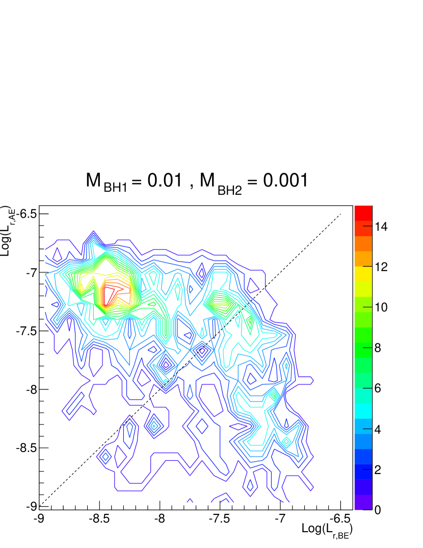
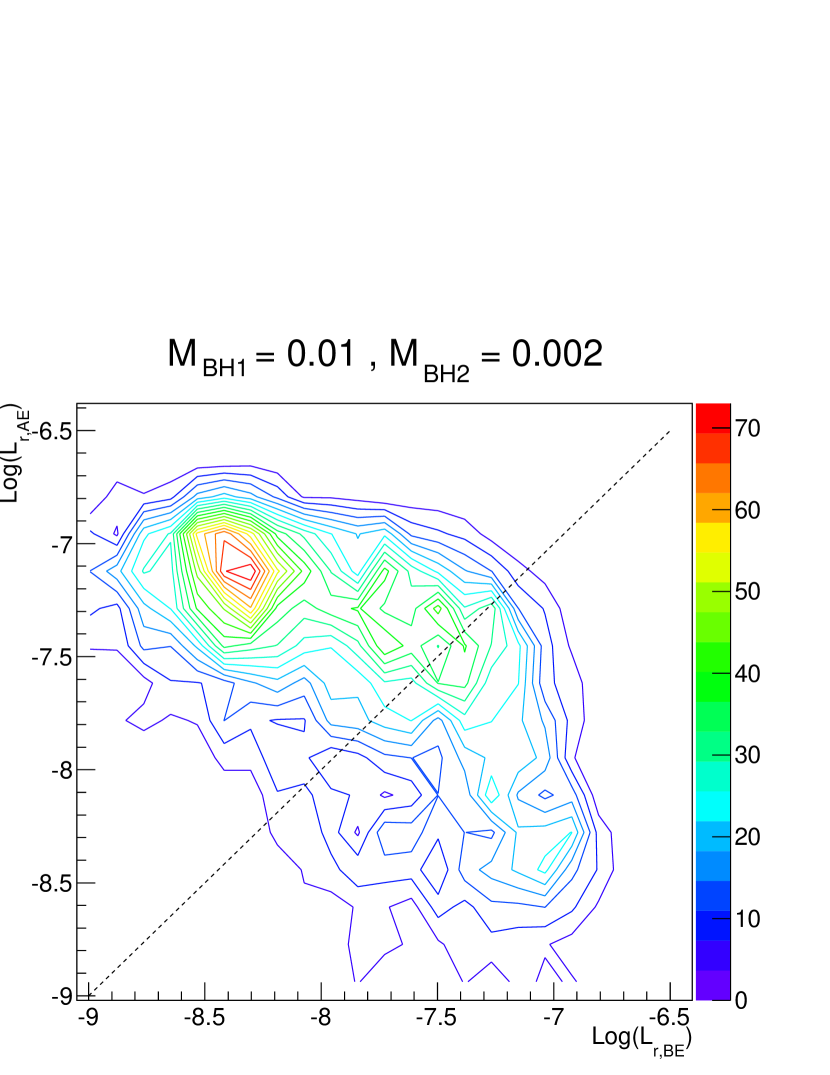
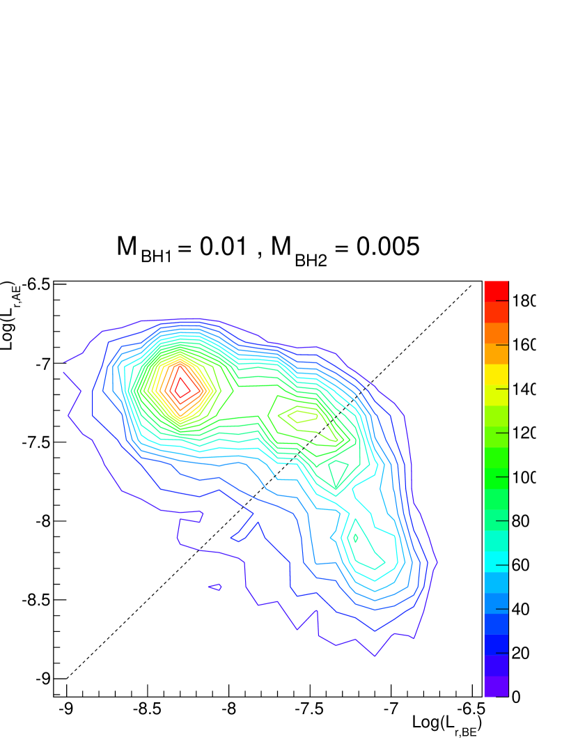
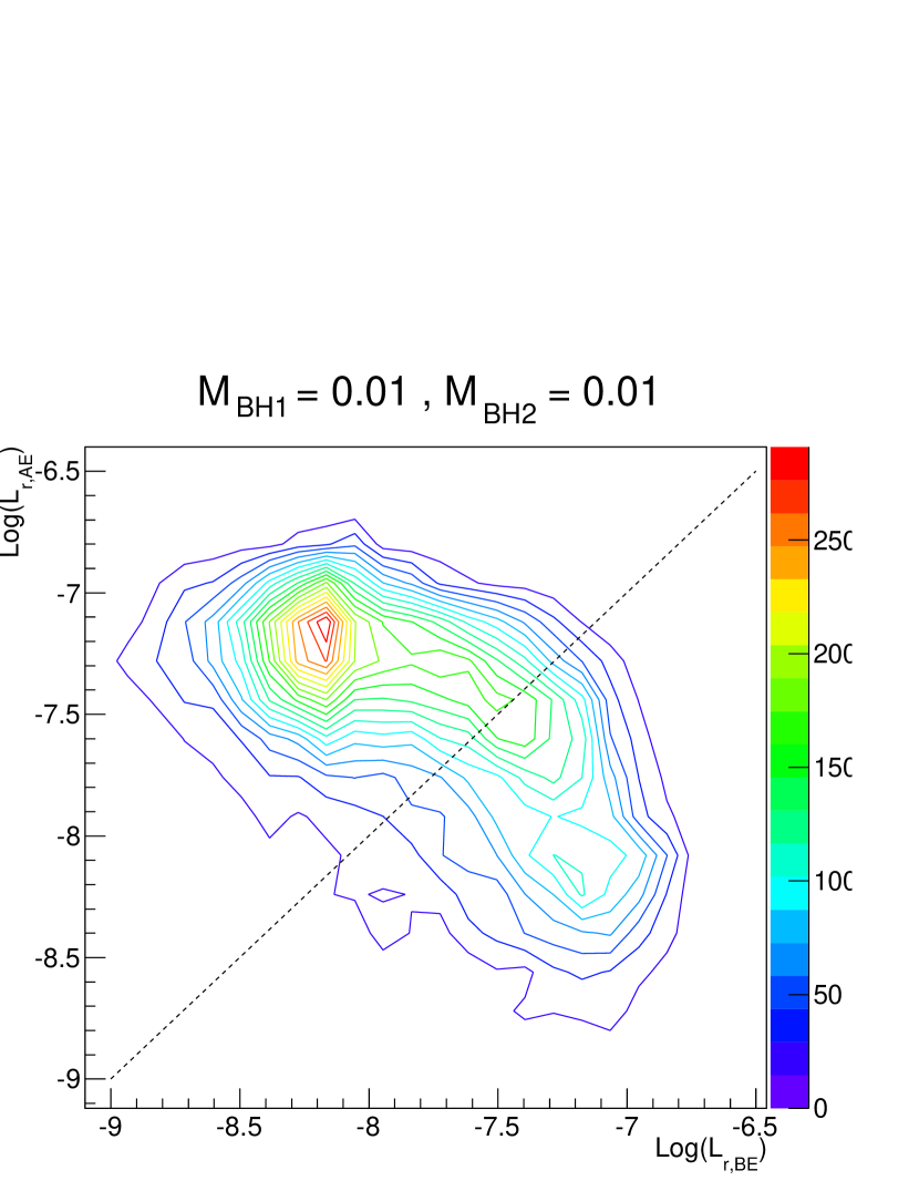
Figure 5: Density maps of logarithmic value of angular momentum of ejected stars ($\log L_{r}$) after vs. before ejection for all models with $t>50$ $N$-body time units. Along the dotted line, $L_{r}$ has no change before and after ejection. The last two panels are non-rotation models for comparison.

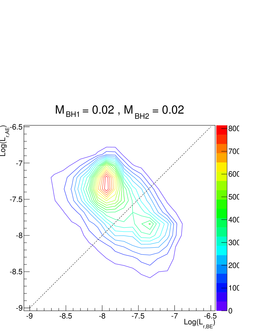
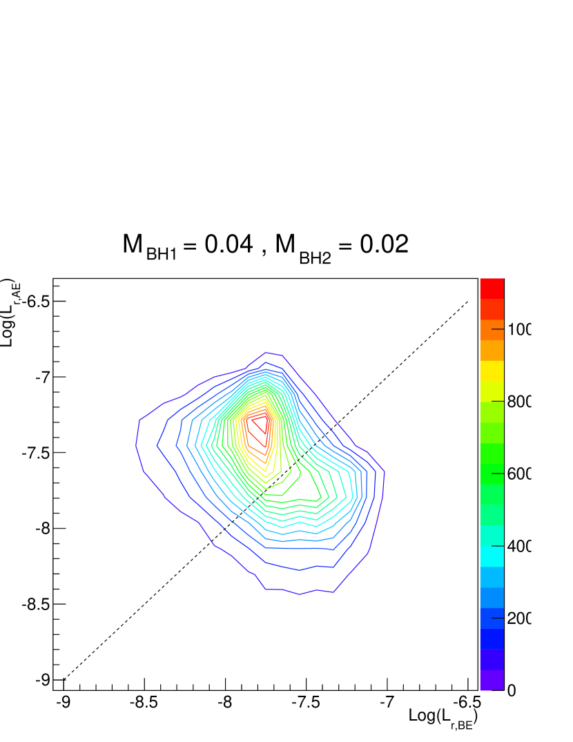
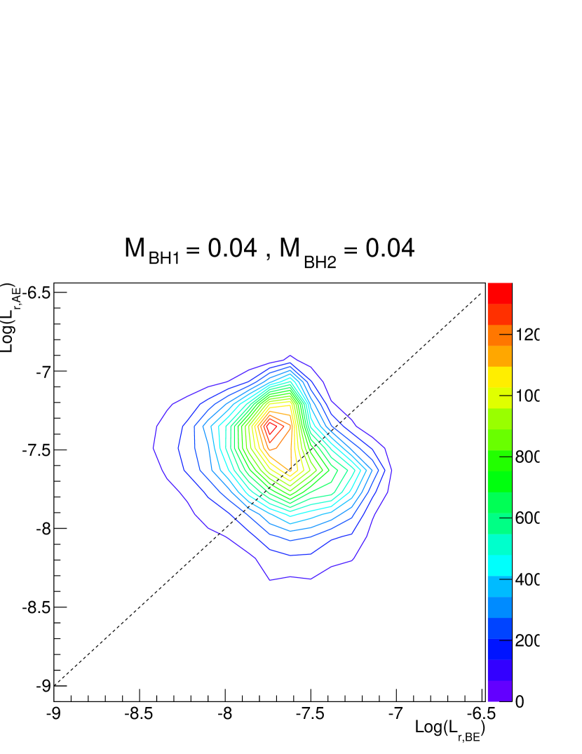
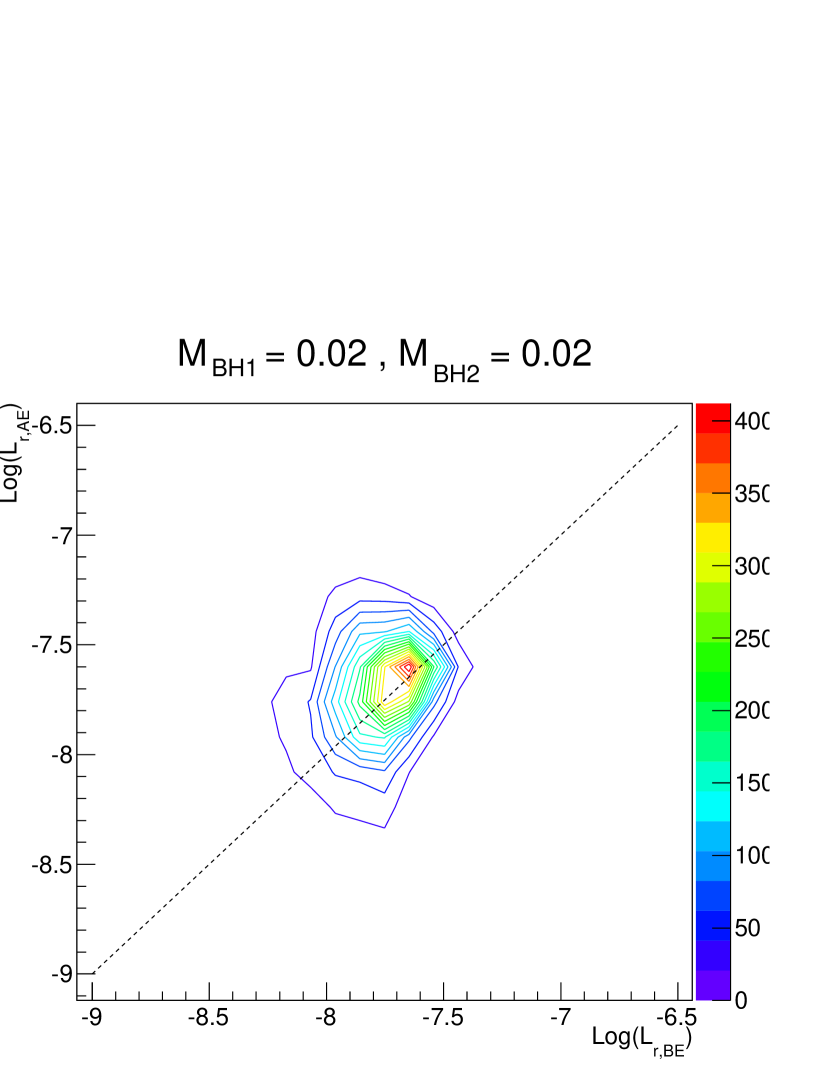
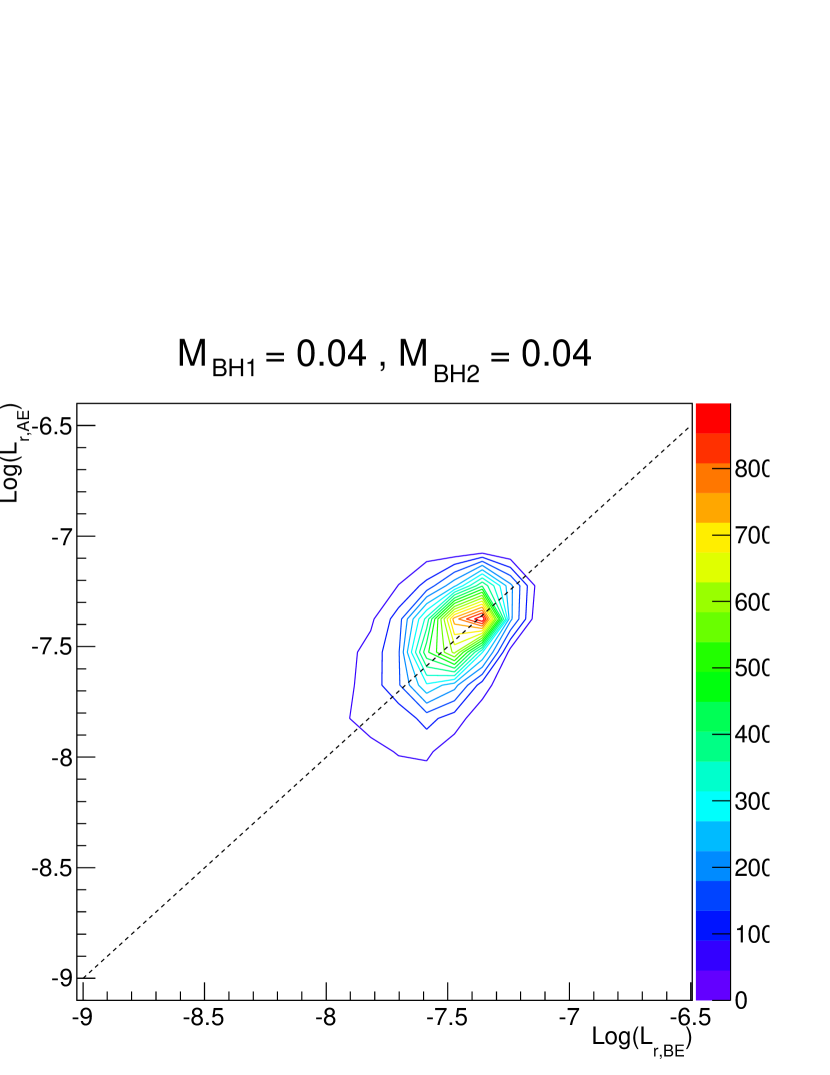
Figure 5: Continue of Figure 5

The angular momentum of individual ejected stars $L_{r,AE}$ as compared to that before ejection $L_{r,BE}$ in all models shows an increasing trend. Figure 5 provides evidence for this trend. If one of the ejected stars gains $L_{r}$ during its ejection, it is located in the top-left region of the density map, and vice versa. We see that there is both gain and loss of $L_{r}$ of ejected stars. But the total $L_{r}$ gain of the ejected stars is larger than the loss since the density peaks are located in the top-left region for all models. This indicates that the ejected stars will carry away net angular momentum from the MBHB. As an additional effect, they also carry away and redistribute some of the angular momentum of the stellar system.

Two more effects are shown in Figure 5. One is that, independent of the mass of the MBHBs, the stellar angular momentum after the encounter $L_{r,AE}$ is approximately constant (it is actually a distribution where the highest level contour lines are nearly flat, parallel to the horizontal axis, which is the angular momentum before the encounter $L_{r,BE}$). This means that stars of any incoming angular momentum get a typical angular momentum after the encounter which is independent of its initial value and is only determined by the properties of the MBHB. The value of such post-encounter angular momentum becomes smaller for larger MBHB mass. In case of the non-rotating stellar system the effect is not visible in the plot, the angular momentum after the encounter scatters in a more symmetric distribution around the line of equality with the initial angular momentum.

4.4.2 Distribution of angular momentum direction

The direction of incoming and ejecting orbits of ejected stars viewed in rectangular coordinate system is influenced by rotational planes of both the whole stellar system and the MBHB. The distribution of $\alpha_{s}$ and $\delta_{s}$ (see Section 4.1) is similar before and after ejection (Figure 6).

For I-Models, the MBHBs have a stable $\alpha_{b}$ and $\delta_{b}$ (e.g., $\alpha_{b}\approx 3.8$ and $\cos(\delta_{b})\approx 0.15$ in model $2020$) (Figure 6), i.e. the direction of the angular momentum of the MBHB binary (or its orbital plane) does not change much during all the stellar encounters. The $\alpha_{s}$ and $\delta_{s}$ distribution concentrates near the same angles or ($\pm\pi$) as the MBHB, both before and after ejection. This indicates that the MBHB interacts preferentially with stars having the same orbital plane. The rotational direction of the stars may be the same or opposite rotational direction as MBHBs’ (co- or counterrotating) and $\cos(\delta_{s})$ also has a concentration towards $0$. Thus ejected stars are oriented with their orbital plane to the one of the MBHB, which is perpendicular to the stellar system rotational symmetry plane (the $x-y$ plane).

For P-Models, the MBHBs orbital plane is close to the $x-y$ plane, aligned with the stellar system’s rotational symmetry plane and $\alpha_{b}$ cannot be defined well. Therefore there is an extended distribution of $\alpha_{b}$ and we expect to see no special trend of $\alpha_{s}$ related to $\alpha_{b}$ (like model $4020$ in Figure 6). The $\cos(\delta_{s})$ distribution also has strong concentration close to $0$ and less concentration on $\cos(\delta_{b})$. The orbits of the ejected stars, which prefer $\cos(\delta_{s})\approx 0$, are now not correlated with the MBHB’s orbital plane, but rather with the stellar system’s rotational symmetry plane. Therefore we see in this case an effect of the rotation of the stellar system, which dominate the orbit direction of ejected stars in P-Models and overrides the MBHBs rotational effect we see in the I-Models.

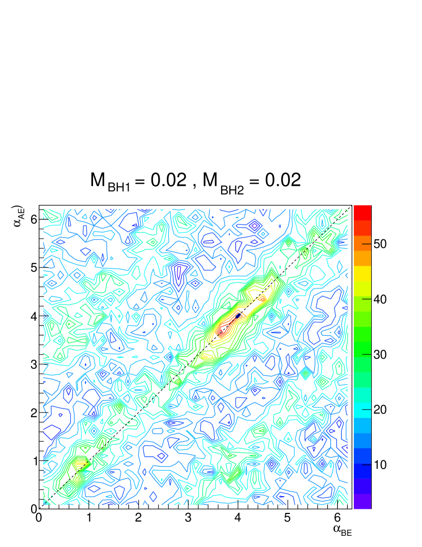
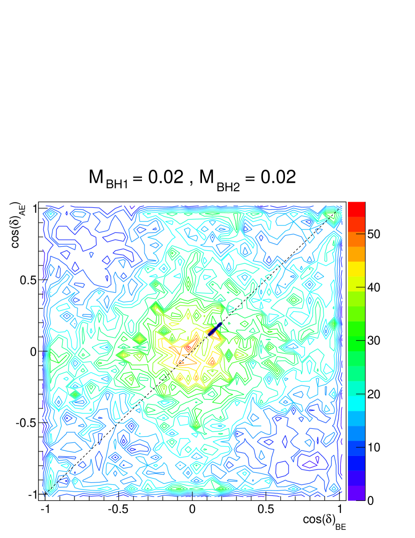
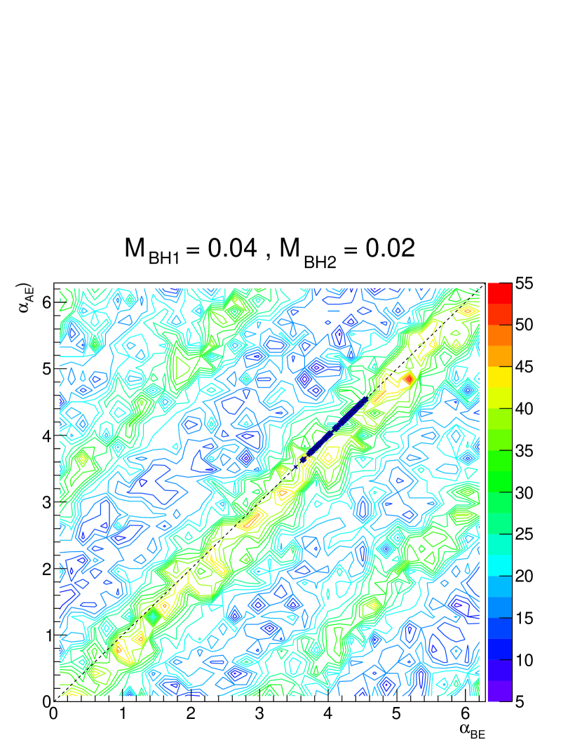
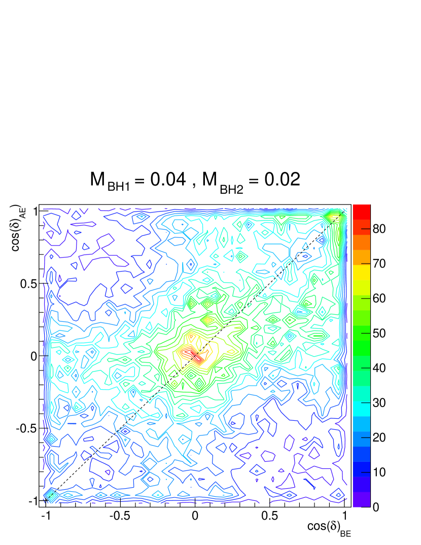
Figure 7: Left: the density map of $\alpha_{AE}$ vs. $\alpha_{BE}$ of ejected stars and MBHBs. Right: the similar map for $\delta$. Here are the same models $2020$ and $4020$ in Figure 6. The colored contour indicate ejected stars and the black contour show MBHBs.

In Figure 7 we use the angles $\alpha_{s}$ and $\delta_{s}$ to illustrate the relation between the stellar orbit before (BE) and after (AE) the encounters. Particularly interesting are the concentrations near the lines $\alpha_{s,AE}-\alpha_{s,BE}=\pm\pi$, which indicates that initially counter-rotating stars (with respect to the MBHB orbital plane) become co-rotating after the encounter and ejection. But the $\alpha_{s,BE}$ and $\alpha_{s,AE}$ in both I-Models and P-Models show also concentrations near the line without change, which means that many ejected stars preserve their rotational direction during the encounter, independent of that of the MBHB. We can also see that $\alpha_{s}$ concentrates near $\alpha_{b}$ with small change before and after ejection in Model $2020$. The $\delta_{s}$ have a wider change than the $\alpha_{s}$ and concentrate near $\delta_{s}=\pi/2$ with a small change.

The information about the relation between incoming and ejected stellar orbital plane, related to the one of the MBHB, can be more easily analyzed by looking at a single angle $\theta$, which is the inclination angle between ejected stars and MBHB (Figure 8). For I-Models, the distribution of $\cos\theta$ is flat (model $1001$, $1002$) with a little increase around $\cos\theta=\pm 1$ (model $2020$). This indicates that ejected stars show a preference of co- and counter-rotation with respect to the MBHBs’ rotation, which is consistent with the results discussed above.

For P-Models, $\cos(\theta_{BE})$ and $\cos(\theta_{AE})$ show clear concentrations near $\pm 1$ and $0$ (slight bias for $\cos(\theta_{AE})$ in model $4040$) . It means that the ejected stars tend to have a incident and ejecting orbits parallel or perpendicular to the MBHB’s rotational orbit in the P-Models, which is consistent with Figure 6.

There is also a slight trend that ejected stars prefer to co-rotate with MBHBs since the fraction of positive $\cos(\theta)$ is larger than the negative fraction.

The distribution $\cos(\theta)$ in models $4040$ and $4020$ also shows a significant difference between before and after ejection (Figure 8) . In these two cases, MBHBs tend to switch orbits of incident stars counter-rotating with MBHBs to co-rotating ones.

For non-rotating models, both $\cos(\theta_{BE})$ and $\cos(\theta_{AE})$ show no trend of concentration near the $-1$ and $0$, but a strong concentration on $1$. This indicates that for non-rotating models, ejected stars prefer to have incident and ejecting orbits co-rotating with MBH’s rotational orbit and also confirms that the concentration near $0$ is the effect of stellar system rotation. There is also the trend of switching orbits of incident stars counter-rotating with MBHBs to co-rotating orbits for rotating models.

5 Conclusions

High accuracy direct $N$-body models of spherical and axisymmetric (rotating) star clusters in galactic nuclei have been presented here, which consist of one million stars and two massive black holes (MBH), which are initially unbound. We study the evolution of a massive black hole binary (MBHB) forming during the evolution and its detailed interactions (superelastic scatterings) with single stars. The two MBHs have three evolutionary phases: the dynamical friction phase, the three-body encounter phase and a final gravitational wave (GW) radiation phase. The MBHs will sink toward the galactic center, form a binary whose orbit shrinks through superelastic three-body encounters until they final coalesce under strong emission of gravitational waves.

Some authors have reported a “Final Parsec Problem” for this three phase MBHB merging scienario purely based on stellar dynamical processes. The timescale of MBHB merging would be too long compared to the evolutionary time scale of galactic nuclei and galaxy mergers, which are the origin of MBHB. The MBHB would stall at a separation of about a parsec with an empty loss cone, no further hardening (orbit shrinking) occurs and relativistic energy losses are yet too small (Begelman et al., 1980).

Currently it seems that the “Final Parsec Problem” only occurs under unphysical idealized conditions, such as a strictly spherical stellar system. Under more general conditions, such as some degree of rotation or triaxiality (bars or tidal fields) or the presence of gas there is no problem to bring an MBHB in few Gyrs to complete relativistic coalescence (Berczik et al., 2005, 2006; Preto et al., 2011; Khan et al., 2011, 2012b, 2012a, 2013).

In this work we have studied the details of the interactions between single stars and the MBHB with an unprecedented detail and statistical quality due to the large particle number in our simulations (obtained with the $\varphi$GPU code on large GPU accelerated supercomputers in China and Germany). The detailed evolution of energy and angular momentum of the MBHB during a large number of slingshot interactions with stars is analyzed. Also the effect of a large scale rotation of the stellar cluster surrounding the MBHB binary is taken into account.

The nuclear stellar cluster surrounding the MBHB is simulated with direct high-accuracy $N$-body simulation (Hermite scheme, $\varphi$GPU  (Berczik et al., 2011) code) with up to $10^{6}$ equal mass stars. A parameter study is presented with different mass ratios of the black holes to each other and to the single stars (see Table 1). We build an efficient method to select the ejected stars from the simulations in order to understand the detailed properties of ejected stars and how they change the eccentricity of the MBHBs when slingshot effects dominate the hardening of the MBHBs. About $0.08\%$ to $8\%$ of stars are ejected by MBHBs in our $150$ $N$-body time unit simulations (see Table 2, if we use the scale factor as discussed in the last part of Section 3, $150$ is about $2.25Gyr$).

Our results (see Figure 4) exhibit two different classes of systems based on the MBHB’s rotational axis direction at the time it becomes gravitationally bound, which we denote as $I$-model (the inclination angle between MBHBs’ orbits and stellar system rotational symmetry plane is large) and $P$-model (MBHBs orbital plane is nearly parallel to the stellar system’s rotational symmetry plane). $I$-model and $P$-model lead to different characteristics of the angular momentum distribution of ejected stars (Figure 6,7,8). The histogram reflects both the rotation of the surrounding star cluster as well as the one of the MBHB - there is a maximum both at angular momenta perpendicular to the orbit of MBHB, and another one aligned with the stellar system (see I-models in Figure 8). If the stellar system is spherically symmetric we only see the maximum at ejected stellar orbits co-rotating with the MHBH (see last two histograms in Figure 8).

Besides, the larger mass MBHBs have a stronger rotational correlation with ejected stars. If the black hole and the stellar system’s rotational symmetry plane are similar, the effect is even stronger. For the $P$-model, the stellar system’s rotational symmetry plane dominates the concentration features of ejected stars (see Figure 6,8).

Finally, we find that massive MBHB (models $4040$ and $4020$ in Figure 8) in both rotating and non-rotating galactic nuclei deplete co-rotating stars, because relatively more ejected stars are co-rotating with the MBHB. This agrees with models of Zier & Biermann (2001, 2002); Iwasawa et al. (2011); Meiron & Laor (2013). Iwasawa et al. (2011) carried out simulations with small mass ratios (1/100) and they only considered bound stars and a non-rotating stellar system. They argue that non-axisymmetric perturbations by the secondary black hole create an effect, which is also seen in our simulations with rotating models containing a massive MBHB and non-rotating models (see Figure 8): initially counter-rotating stars become co-rotating after being scattered. Our results show this effect for much more general conditions (up to equal mass ratio of the MBHB and including mostly unbound scattered stars). The average eccentricity changes of our MBHBs agree fairly well with early Monte Carlo prediction (Quinlan, 1996) (see Figure 3), but the scatter for individual events is quite large. This means that our interactions, detected in the numerical simulations, cover a different, and we think more realistic range of encounters than used in the early investigation of Quinlan (1996). This could be due to different distributions of relative velocities, impact parameters or the movement of the MBHB. This effect is more pronounced for the few cases where we have low eccentricity, while for the large $e$ our results follow the same trend as Quinlan (1996). Our data show that the eccentricity grows in a stochastic way, where positive and negative $K$ occur all the time, but there is an average trend towards higher eccentricity. The relativistic Post-Newtonian evolution of the MBHB and its gravitational wave emission in the final phase before coalescence depends on such detailed orbital evolution, which is a reason why we need simulations like ours and others for a correct assessment of gravitational radiation from MBHB in the universe (cf. e.g. Preto et al. (2011); Khan et al. (2011, 2013)). We obtain an average higher eccentricities as comparied to Khan et al. (2013). The reason for this is probably that we have rotating models while their galaxy models are non-rotating.

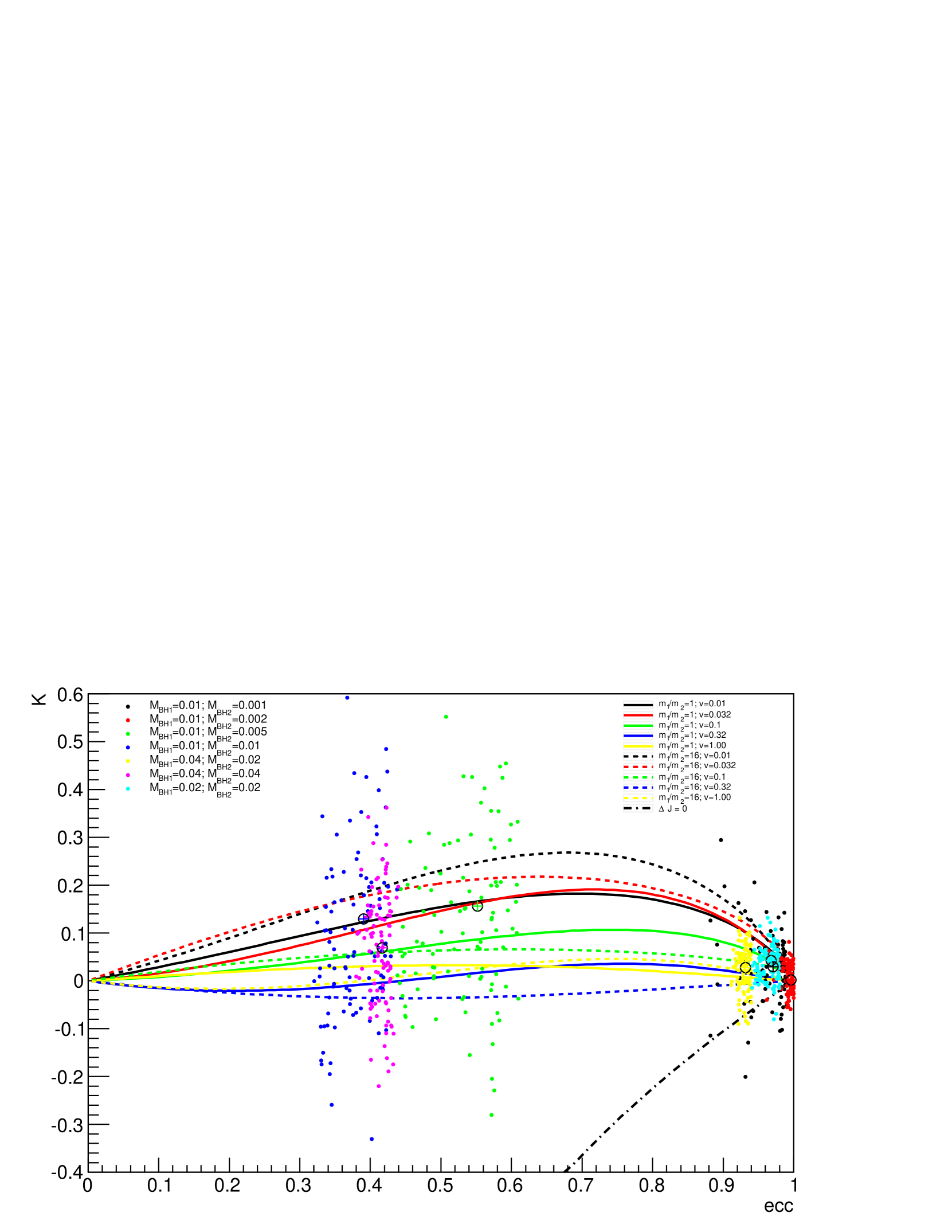
Figure 3: The eccentricity growth rate $K$ vs. eccentricity $e$ for all rotating models. Points are calculated results using Equation 4. Circles with crosses are average $K$ between $t=81$ $N$-body units to the end of simulation. Solid and dashed curves are fitted function for $K_{1}$ from Quinlan (1996). Here $v$ represents $v/V_{bin}$ in Quinlan (1996).

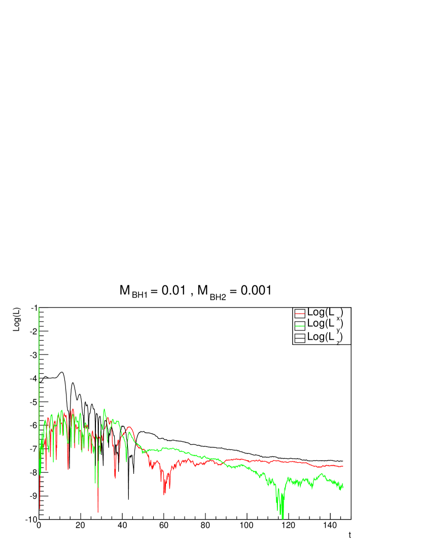
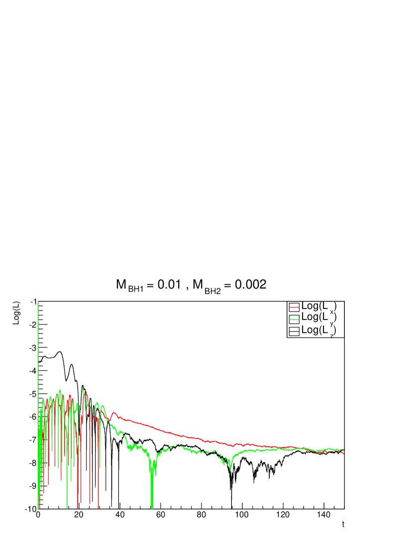
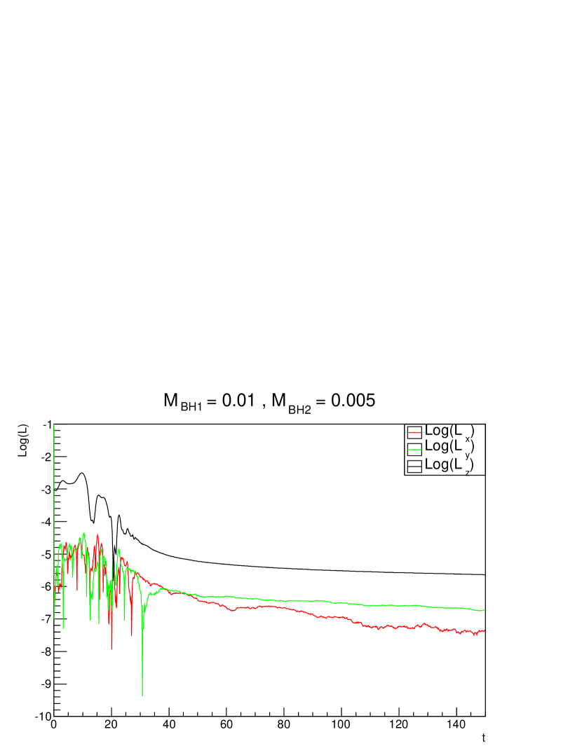
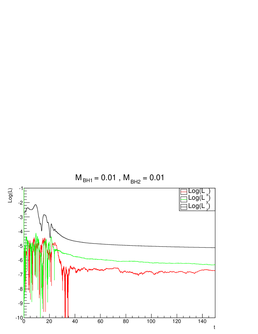
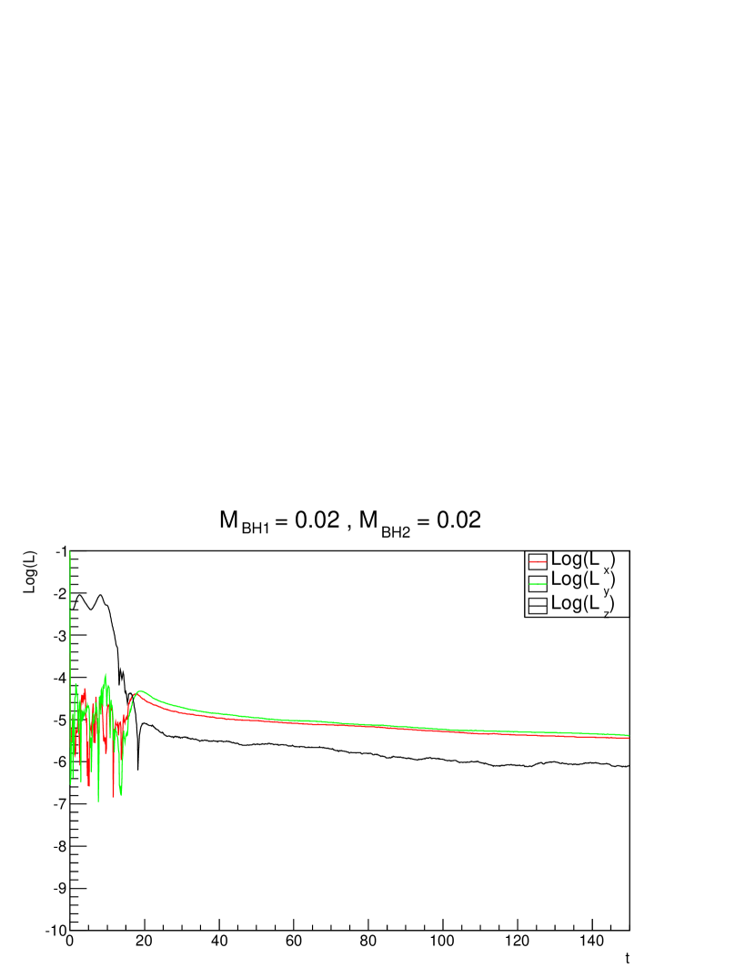
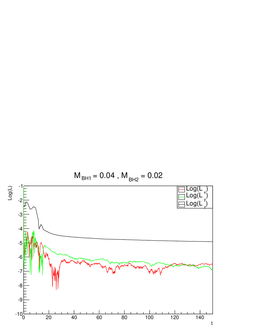
Figure 4: The evolution of each components $L_{x}$ (red), $L_{y}$ (green) and $L_{z}$ (black) of the MBHBs angular momentum(Section 4.1). The last two panels are non-rotation models for comparison. Due to the inclination between the MBHB’s orbit and stellar system’s rotational symmetry plane, models $1001$, $1002$ and $2020$ are classified as I-models and all others are classified as P-models

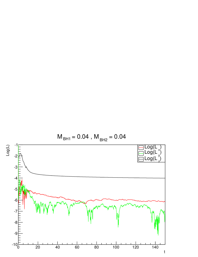
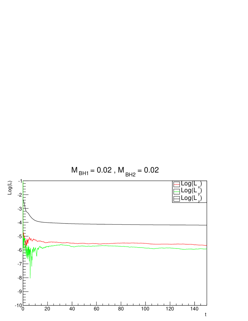
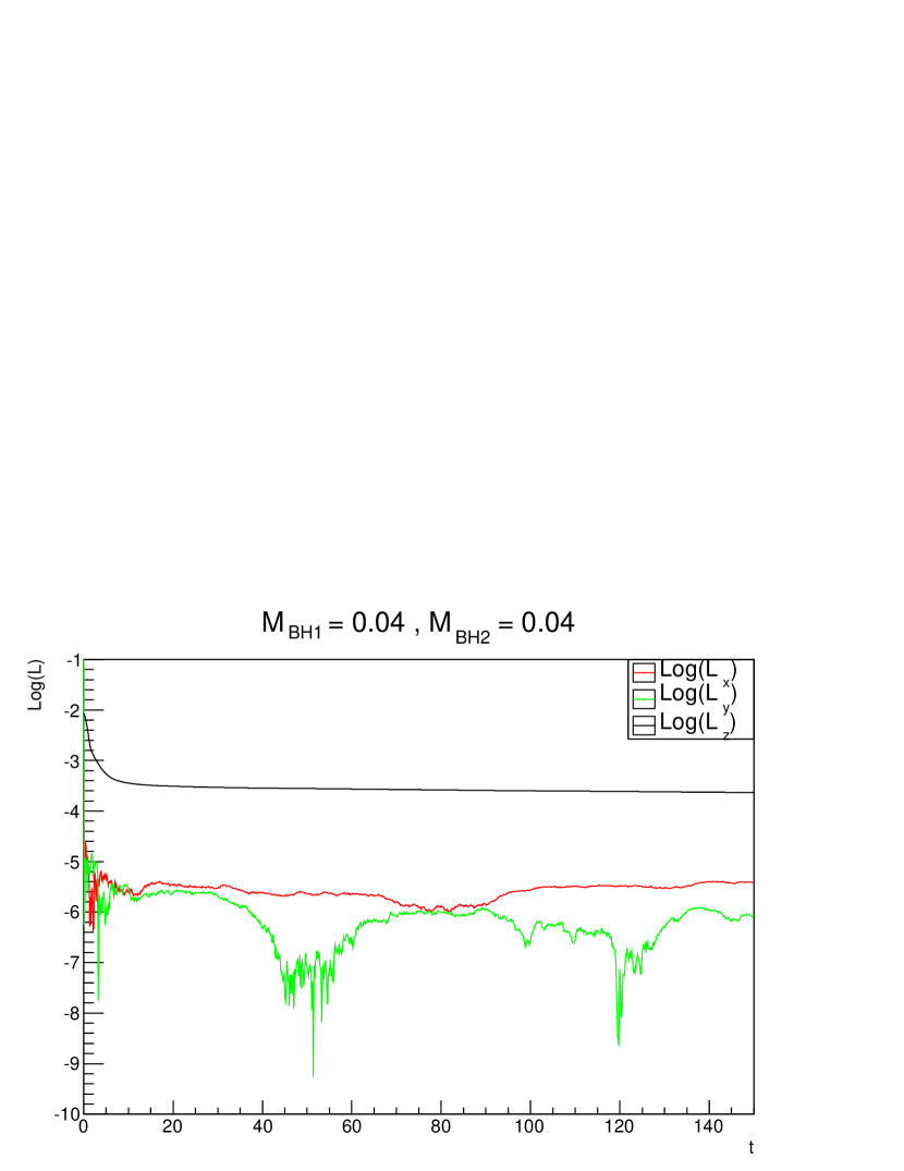
Figure 4: Continue of Figure 4

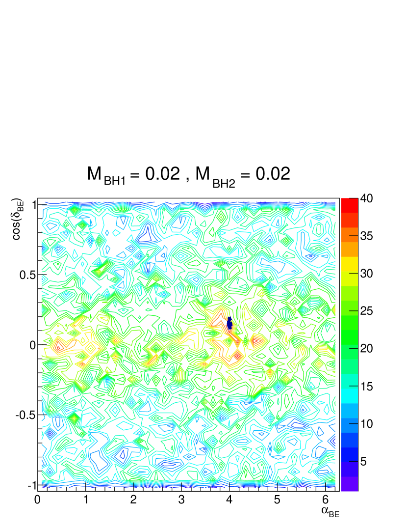
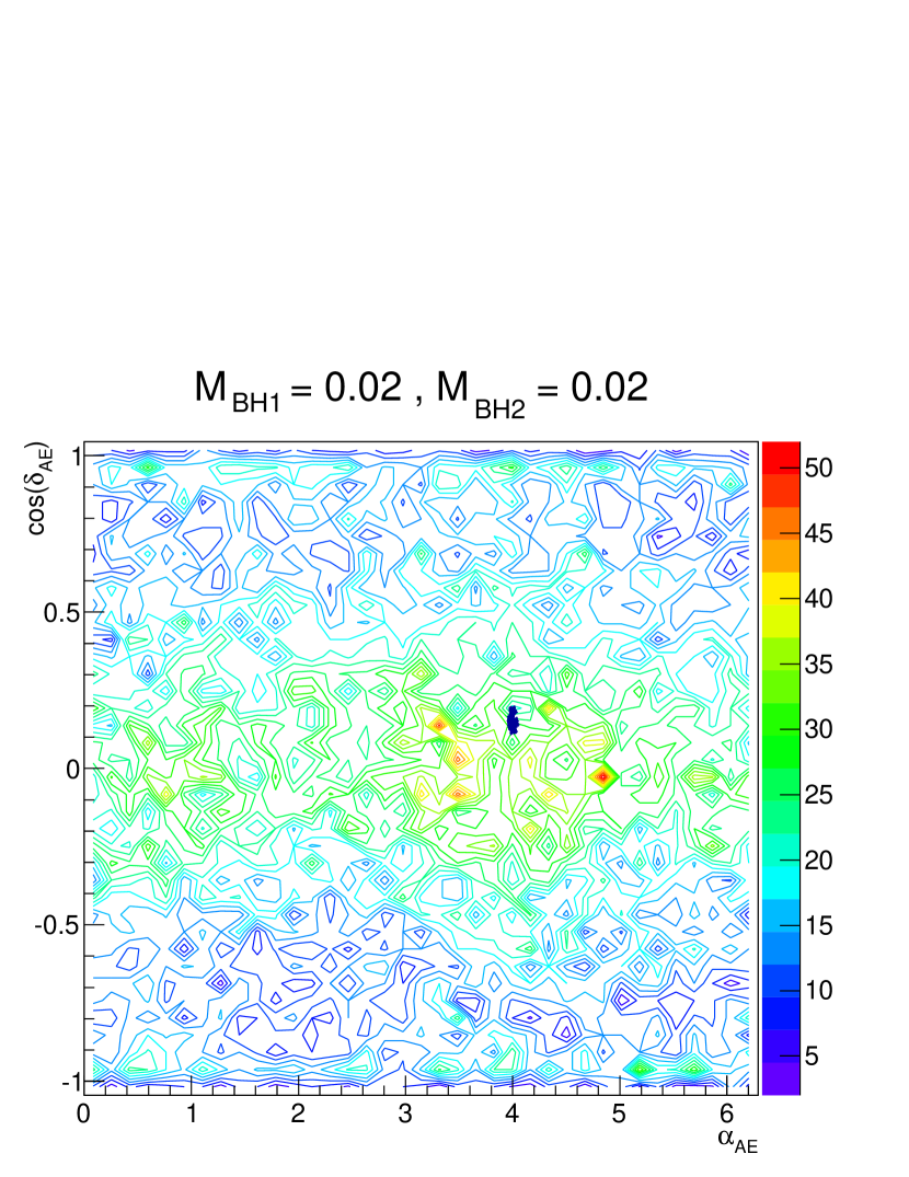
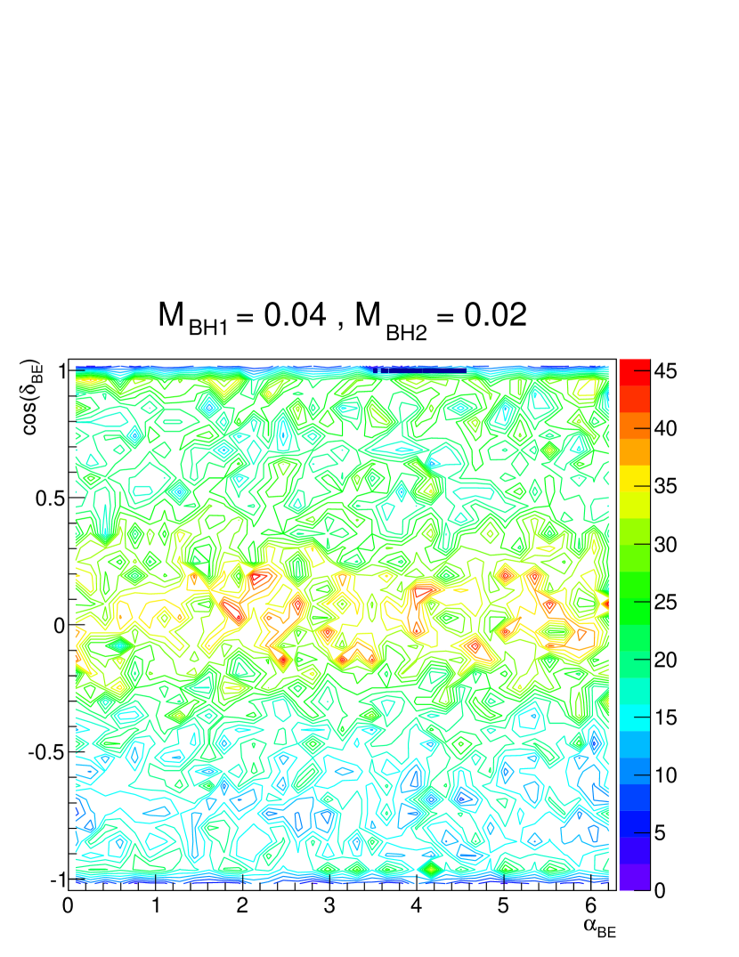
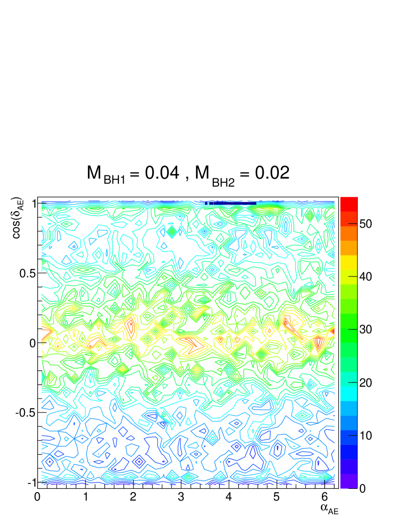
Figure 6: Density maps of $\delta$ vs. $\alpha$ of ejected stars and MBHBs with $t>50$ $N$-body time unit before (left) and after (right) ejection The top two panels represent model $2020$ (I-model) and the bottom two panels represent model $4020$ (P-model). The colors of the contours represent ejected stars and black points and lines (near center in top panels and near top edge in the bottom panels ) represent the MBHBs.

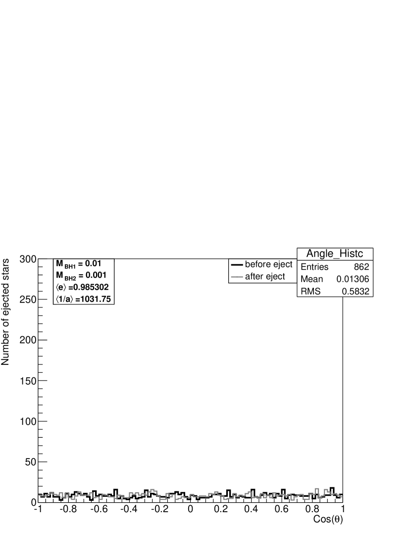
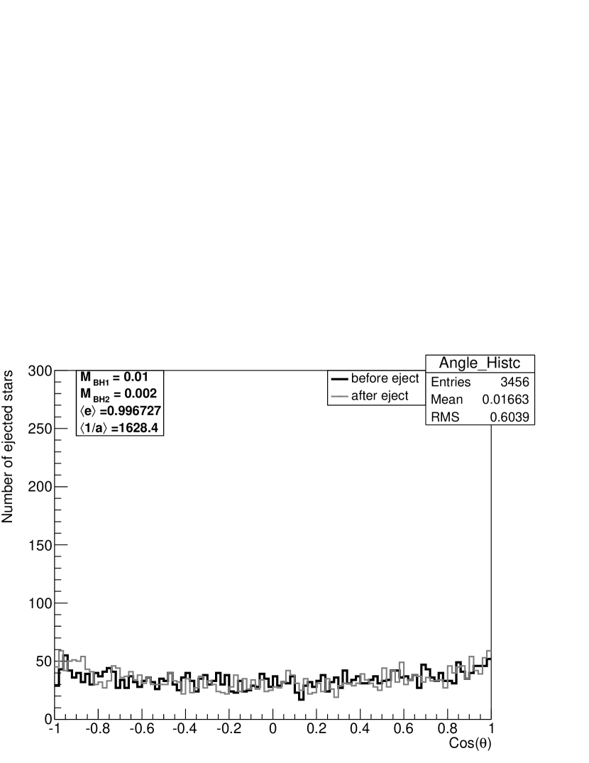
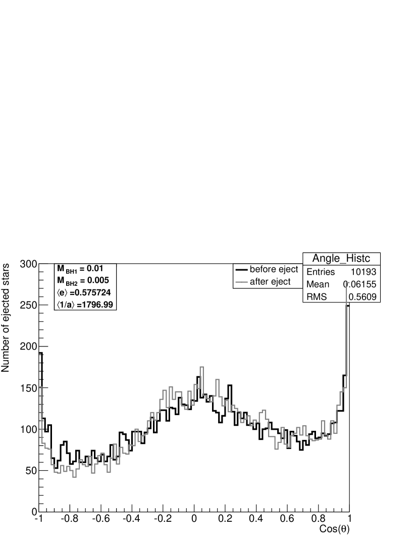
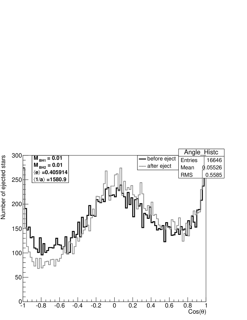
Figure 8: The distribution of $\cos(\theta)$ before and after ejection. In each sub-diagram, we also show the average eccentricity $\left\langle e\right\rangle$ and $\left\langle 1/a\right\rangle$ of MBHBs during time $100$ to $150$ in $N$-body units, where $a$ is semi-major axis of MBHBs. The last two panels are non-rotation models for comparison.

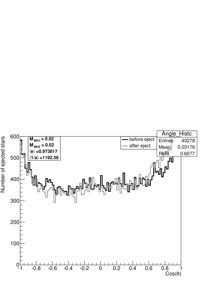
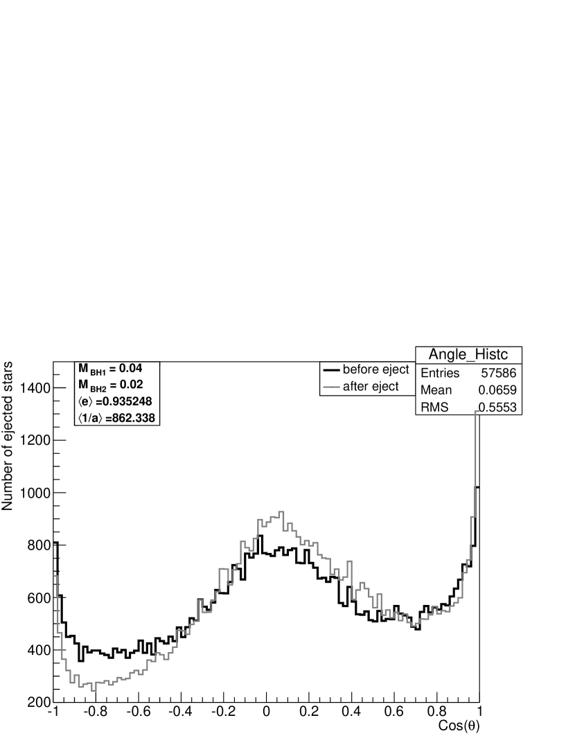
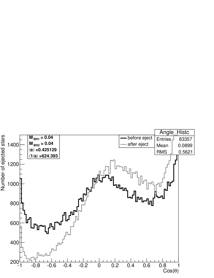
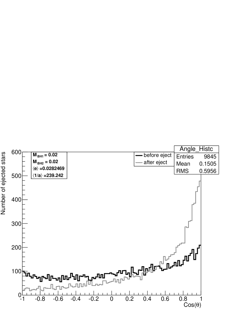
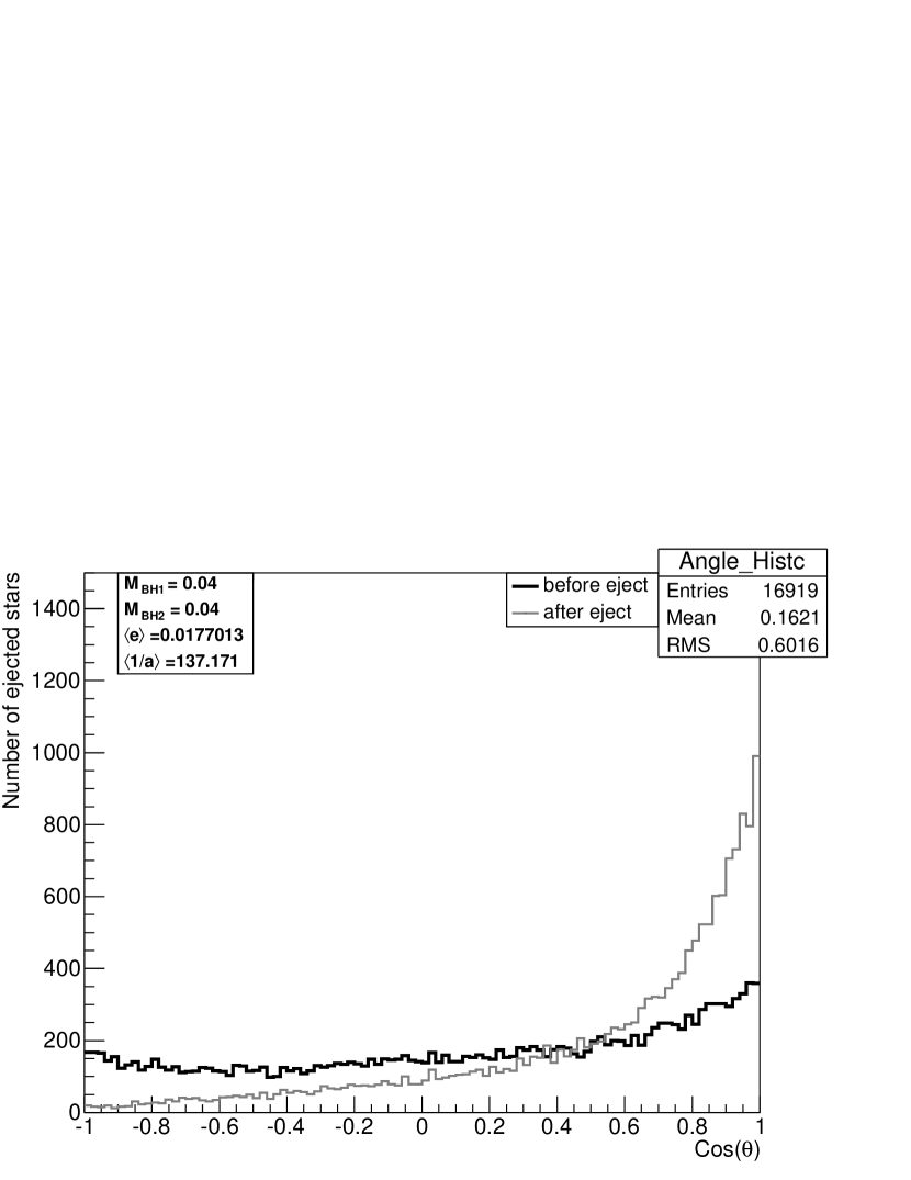
Figure 8: Continue of Figure 8

References

- Aarseth (2003) Aarseth, S. J. 2003, Ap&SS, 285, 367
- Aarseth et al. (1974) Aarseth, S. J., Henon, M., & Wielen, R. 1974, A&A, 37, 183
- Amaro-Seoane et al. (2010) Amaro-Seoane, P., Sesana, A., Hoffman, L., et al. 2010, MNRAS, 402, 2308
- Begelman et al. (1980) Begelman, M. C., Blandford, R. D., & Rees, M. J. 1980, Nature, 287, 307
- Berczik et al. (2005) Berczik, P., Merritt, D., & Spurzem, R. 2005, ApJ, 633, 680
- Berczik et al. (2006) Berczik, P., Merritt, D., Spurzem, R., & Bischof, H.-P. 2006, ApJ, 642, L21
- Berczik et al. (2011) Berczik, P., Nitadori, K., Zhong, S., et al. 2011, in High Performence Computing HPC-UA, Vol. 4, 8
- Berczik et al. (2013a) Berczik, P., Spurzem, R., Berentzen, I., & Nitadori, K. 2013a, ApJ, will be submitted
- Berczik et al. (2013b) Berczik, P., Spurzem, R., Zhong, S., et al. 2013b, in Lecture Notes in Computer Science, Vol. 7905, Procs. of 28th Intl. Supercomputing Conf. ISC 2013, Leipzig, Germany, June 16-20, 2013., ed. J. M. Kunkel, T. Ludwig, & H. E. Meuer (Springer Vlg.), 13–25
- Berentzen et al. (2008) Berentzen, I., Preto, M., Berczik, P., Merritt, D., & Spurzem, R. 2008, Astronomische Nachrichten, 329, 904
- Berentzen et al. (2009a) —. 2009a, ApJ, 695, 455
- Berentzen et al. (2009b) —. 2009b, ApJ, 695, 455
- Einsel & Spurzem (1999) Einsel, C., & Spurzem, R. 1999, MNRAS, 302, 81
- Fiestas et al. (2012) Fiestas, J., Porth, O., Berczik, P., & Spurzem, R. 2012, MNRAS, 419, 57
- Fukushige et al. (2005) Fukushige, T., Makino, J., & Kawai, A. 2005, PASJ, 57, 1009
- Gong et al. (2011) Gong, X., Xu, S., Bai, S., et al. 2011, Classical and Quantum Gravity, 28, 094012
- Greene & Ho (2009) Greene, J. E., & Ho, L. C. 2009, PASP, 121, 1167
- Gualandris et al. (2012) Gualandris, A., Dotti, M., & Sesana, A. 2012, MNRAS, 420, L38
- Gualandris & Merritt (2012) Gualandris, A., & Merritt, D. 2012, ApJ, 744, 74
- Harfst et al. (2007) Harfst, S., Gualandris, A., Merritt, D., et al. 2007, New A, 12, 357
- Iwasawa et al. (2011) Iwasawa, M., An, S., Matsubayashi, T., Funato, Y., & Makino, J. 2011, ApJ, 731, L9
- Khan et al. (2013) Khan, F., Holley-Bockelmann, K., Berczik, P., & Just, A. 2013, ApJ, 773, 100
- Khan et al. (2012a) Khan, F. M., Berentzen, I., Berczik, P., et al. 2012a, ApJ, 756, 30
- Khan et al. (2011) Khan, F. M., Just, A., & Merritt, D. 2011, ApJ, 732, 89
- Khan et al. (2012b) Khan, F. M., Preto, M., Berczik, P., et al. 2012b, ApJ, 749, 147
- Li et al. (2012) Li, S., Liu, F. K., Berczik, P., Chen, X., & Spurzem, R. 2012, ApJ, 748, 65
- Lu et al. (2010) Lu, Y., Zhang, F., & Yu, Q. 2010, ApJ, 709, 1356
- Meiron & Laor (2013) Meiron, Y., & Laor, A. 2013, ArXiv e-prints
- Merritt (2001) Merritt, D. 2001, ApJ, 556, 245
- Merritt & Poon (2004) Merritt, D., & Poon, M. Y. 2004, ApJ, 606, 788
- Milosavljević & Merritt (2003) Milosavljević, M., & Merritt, D. 2003, ApJ, 596, 860
- Nitadori & Makino (2008) Nitadori, K., & Makino, J. 2008, New A, 13, 498
- Peters (1964) Peters, P. C. 1964, Physical Review, 136, 1224
- Preto et al. (2009) Preto, M., Berentzen, I., Berczik, P., Merritt, D., & Spurzem, R. 2009, Journal of Physics Conference Series, 154, 012049
- Preto et al. (2011) Preto, M., Berentzen, I., Berczik, P., & Spurzem, R. 2011, ApJ, 732, L26
- Quinlan (1996) Quinlan, G. D. 1996, New A, 1, 35
- Quinlan & Hernquist (1997) Quinlan, G. D., & Hernquist, L. 1997, New A, 2, 533
- Sesana et al. (2011) Sesana, A., Gualandris, A., & Dotti, M. 2011, MNRAS, 415, L35
- Spurzem et al. (2011a) Spurzem, R., Berczik, P., Berentzen, I., et al. 2011a, in Large Scale Computing Techniques for Complex Systems and Simulations, ed. W. Dubitzky, K. Kurowski, & B. Schott, Wiley Publishers, 35–58
- Spurzem et al. (2012) Spurzem, R., Berczik, P., Zhong, S., et al. 2012, in Astronomical Society of the Pacific Conference Series, Vol. 453, Advances in Computational Astrophysics: Methods, Tools, and Outcome, ed. R. Capuzzo-Dolcetta, M. Limongi, & A. Tornambè, 223
- Spurzem et al. (2011b) Spurzem, R., Berczik, P., Hamada, T., et al. 2011b, Computer Science - Research and Development (CSRD), 26, 145
- Volonteri et al. (2003) Volonteri, M., Haardt, F., & Madau, P. 2003, ApJ, 582, 559
- Yu (2002) Yu, Q. 2002, MNRAS, 331, 935
- Yu & Tremaine (2003) Yu, Q., & Tremaine, S. 2003, ApJ, 599, 1129
- Zier & Biermann (2001) Zier, C., & Biermann, P. L. 2001, A&A, 377, 23
- Zier & Biermann (2002) —. 2002, A&A, 396, 91
(a)
(b)