Transport coefficients of nuclear matter in neutron star cores

Abstract

We calculate thermal conductivity and shear viscosity of nucleons in dense nuclear matter of neutron star cores in the non-relativistic Brueckner-Hartree-Fock framework. Nucleon-nucleon interaction is described by the Argonne v18 potential with addition of the Urbana IX effective three-body forces. We find that this three body force leads to decrease of the kinetic coefficients with respect to the two-body case. The results of calculations are compared with electron and muon transport coefficients as well as with the results of other authors.

I Introduction

Kinetic coefficients of neutron star cores are important ingredients in modeling of various processes in neutron stars. As the most dense stars in the Universe (with densities exceeding nuclear density $\rho_{0}\approx 2.8\times 10^{14}$ g/cm³) neutron stars are widely considered as unique laboratories for studying properties of super-dense matter under the extreme conditions unavailable in terrestrial laboratories. Due to this reason studies of neutron stars attract constant interest.

It is believed that a neutron star consists of the dense core filled with uniform asymmetric nuclear matter surrounded by the thin crust (for example, Haensel et al. (2007)). The outer part of the core contains neutrons with small admixture of protons, and electrons and muons as charge-neutralizing component. The equation of state and composition of inner parts of neutron stars are poorly known. The different possibilities, apart from the nuclear matter, are: hyperon core, kaon or pion condensates, quark core. It is possible that all or some neutron stars are in fact so-called strange stars containing self-bound strange quark matter.

In what follows we restrict ourselves to the simplest model of the nucleon neutron star core which consists of neutrons (n), protons (p), electrons (e), and muons ($\mu$). The nuclear matter is in the equilibrium state with respect to the beta-processes, which is commonly called beta-stable nuclear matter.

In the present paper we consider shear viscosity and thermal conductivity of the neutron star cores. The thermal conductivity is needed for modeling thermal structure and evolution of such stars. It is especially important for studying cooling of young neutron stars (age $\lesssim 100$ yr) where the internal thermal relaxation is not yet finished (e.g., Gnedin et al. (2001); Shternin and Yakovlev (2008a)). Shear viscosity is important for studying decay of the oscillations of neutron stars and stability of rotating stars (e.g. Andersson and Kokkotas (2001)).

The diffusive kinetic coefficients are governed by the particle collisions. The first detailed studies of the kinetic coefficients in neutron star cores were made by Flowers and Itoh Flowers and Itoh (1979). They considered n-p-e matter taking into account collisions between all particle species. Flowers and Itoh constructed the exact solution of the multicomponent system of transport equations. The small amount of protons and small magnitude of the electron-neutron interaction lead to the conclusion that the kinetic coefficients can be split in two almost independent parts – the neutron kinetic coefficients mediated by nucleon-nucleon collisions and electron kinetic coefficients mediated by the collisions between charged particles; the proton kinetic coefficients are small. The up-to-date electron and muon contribution to kinetic coefficients of neutron star cores was calculated by Shternin and Yakovlev Shternin and Yakovlev (2007) (thermal conductivity) and Shternin and Yakovlev (2008b) (shear viscosity). Here we will focus on the neutron kinetic coefficients.

Flowers and Itoh Flowers and Itoh (1979) based their calculations on the free nucleon scattering amplitudes, which were derived from the experimentally determined phase shifts. They neglected the Fermi-liquid effects and nucleon many-body effects. The results of Flowers and Itoh Flowers and Itoh (1979) were later reconsidered in Refs. Baiko et al. (2001); Shternin and Yakovlev (2008b); Baiko and Haensel (1999). In latter works it was assumed that the main medium effects are incorporated in the effective masses, while the free-space nucleon potential was used.

However in a strongly interacting dense matter the many-body effects play most important role. These effects in the context of transport coefficients of pure neutron matter were first addressed in Refs. Wambach et al. (1993); Sedrakian et al. (1994). In Ref. Wambach et al. (1993) the attempt of a consistent many-body consideration of the kinetic coefficients on the basis of Fermi-liquid theory was made. Authors of Ref. Sedrakian et al. (1994) used the concept of thermodynamical $T$-matrix, neglecting Fermi-liquid effects.

A decade later the medium modifications of the neutron star matter transport coefficients were reconsidered in Refs. Benhar and Valli (2007); Carbone and Benhar (2011); Zhang et al. (2010); Benhar et al. (2010) on the basis of modern realistic nucleon interactions. Different approaches were used. In Ref. Benhar and Valli (2007) the correlated basis function (CBF) formalism were incorporated to obtain the shear viscosity of pure neutron matter. Later the same group Benhar et al. (2010) compared the transport coefficients obtained from CBF and the Brueckner-Hartree-Fock (BHF) $G$-matrix formalism in pure neutron matter and found a good agreement between the results of both approaches; Carbone and Benhar Carbone and Benhar (2011) used CBF formalism to calculate transport coefficients of beta-stable nuclear matter which is directly related to the neutron star properties. Zhang et al. Zhang et al. (2010) calculated the transport coefficients in the framework of the BHF theory.

The general result of Refs. Benhar and Valli (2007); Carbone and Benhar (2011); Zhang et al. (2010); Benhar et al. (2010) is that the medium effects strongly increase the values of kinetic coefficients.

In the present paper we reconsider the problem of the nucleon kinetic coefficients in the dense mater in beta equilibrium in the BHF framework. Generally, our approach is similar to that used by Zhang et al. Zhang et al. (2010). The difference within the approaches will be emphasized below.

The paper is organized as follows. We start from outlining the formalism for calculating the kinetic coefficients in multi-component Fermi-liquid (Section II). In Sec. III we discuss the adopted model of the nucleon interaction and calculate the in-medium nucleon-nucleon cross-sections. We discuss the results and compare them with those by other authors in Sec. IV. Our conclusions are presented in Sec. V.

II Kinetic coefficients

Let us shortly describe the expressions needed to obtain the kinetic coefficients. The transport properties of strongly interacting matter are customary described in the framework of Landau Fermi-liquid theory (e.g., Baym and Pethick (1991)). Consider a multicomponent Fermi-liquid which consists of quasiparticles of different species c with distribution functions $F_{c}(\mathbf{p}_{c})$, where $\mathbf{p}_{c}$ is the quasiparticle momentum. In equilibrium quasiparticle distribution functions are given by the Fermi-Dirac function

$$F_{c}(\mathbf{p}_{c})=f_{c}(\mathbf{p}_{c})=\left[1+\exp\left(\frac{\epsilon_{c}(\mathbf{p}_{c})-\mu_{c}}{k_{B}T}\right)\right]^{-1},$$ (1)

where $\epsilon_{c}(\mathbf{p}_{c})$ is the quasiparticle energy, $\mu_{c}$ is its chemical potential, $T$ is the temperature, and $k_{B}$ is the Boltzmann constant. When perturbations, such as gradients of temperature or a hydrodynamical velocity $\mathbf{V}$, are applied to the system, distribution functions start to deviate from equilibrium ones. It is convenient to present perturbed distribution function in the form

$$F_{c}=f_{c}-\Phi_{c}\frac{\partial f_{c}}{\partial\epsilon_{c}},$$ (2)

where functions $\Phi_{c}$ describe this deviation. These functions depend on quasiparticle quantum numbers and on the type of the perturbation applied to the system. In order to find $\Phi_{c}$ one solves multicomponent system of linearized kinetic equations, which has the following form for the problems of thermal conductivity $\kappa$ and shear viscosity $\eta$

$$\left.\begin{array}[]{ll}\kappa:&(\epsilon_{1}-\mu_{1}){\bf v}_{1}\nabla T/T\\ \eta:&\left(v_{1\alpha}p_{1\beta}-\frac{1}{3}\delta_{\alpha\beta}v_{1}p_{1}\right)V_{\alpha\beta}\end{array}\right\}\frac{\partial f_{1}}{\partial\epsilon_{1}}=\sum_{i}I_{ci}(12;1^{\prime}2^{\prime}),$$ (3)

where $v_{1}$ is the quasiparticle velocity and $V_{\alpha\beta}$ is the rate of strain tensor. The latter tensor is defined as Lifshits and Pitaevskii (1981)

$$V_{\alpha\beta}=\frac{1}{2}\left(\frac{\partial V_{\alpha}}{\partial x_{\beta}}+\frac{\partial V_{\beta}}{\partial x_{\alpha}}\right),\qquad\alpha,\ \beta=x,\,y,\,z,$$ (4)

where it is assumed that $\mathrm{div}\mathbf{V}=0$. The right-hand side in Eq. (3) contains the sum of the linearized Boltzmann collision integrals describing collisions of quasiparticles of species c and i:

$$I_{ci} = \frac{1}{(1+\delta_{ci})k_{B}T}\sum_{\sigma_{1^{\prime}}\sigma_{2}\sigma_{2^{\prime}}}\int\int\int\frac{{\rm d}\mathbf{p}_{1^{\prime}}{\rm d}\mathbf{p}_{2}{\rm d}\mathbf{p}_{2^{\prime}}}{(2\pi\hbar)^{9}}w_{ci}(12;1^{\prime}2^{\prime})f_{1}f_{2}(1-f_{1^{\prime}})(1-f_{2^{\prime}})$$ (5)

$$\times\left(\Phi_{1^{\prime}}+\Phi_{2^{\prime}}-\Phi_{1}-\Phi_{2}\right),$$

where $w_{ci}(12;1^{\prime}2^{\prime})$ is the differential transition rate. Here by labels 1 and 2 we, as usual, denote quasiparticle states before collisions, while the labels with primes correspond to the final states. Once the functions $\Phi_{c}$ are found, the thermal conductivity and shear viscosity are obtained from the expressions for the heat current and the dissipative part of the stress tensor, respectively. These coefficients can be written as

$$\kappa_{c}=\frac{\pi^{2}Tn_{c}\tau^{(\kappa)}_{c}}{3m_{c}^{*}},$$ (6)

$$\eta_{c}=\frac{n_{c}p_{\rm Fc}^{2}\tau_{c}^{(\eta)}}{5m^{*}_{c}},$$ (7)

where $n_{c}$ is the number density of particles of the c species, $m^{*}_{c}$ is their effective mass at the Fermi surface, and effective relaxation times $\tau^{(\kappa)}_{c}$ and $\tau^{(\eta)}_{c}$ are introduced, which are determined by $\Phi_{c}$ functions.

In the limit of low temperatures, all quasiparticles can be placed on the Fermi surface where possible. In addition is it assumed that the transition probability is independent of the energy transferred in the collision event. The exact solution of the kinetic equation for one-component Fermi-liquid in form of rapidly converging series were constructed by Brooker and Sykes Brooker and Sykes (1968); Sykes and Brooker (1970) and Højgård Jensen et al. Højgård Jensen et al. (1968). For multicomponent system the exact solution were given by Flowers and Itoh Flowers and Itoh (1979). Later this approach was further developed in Ref. Anderson et al. (1987). However in order to study general behavior of kinetic coefficients it is enough to employ much simpler variational solution of the system of kinetic equations and introduce correction factors needed to obtain the exact solution. Mathematically, variational solution corresponds to the first term in the series expansion of the full solution Baym and Pethick (1991). Below we show that for nuclear matter the difference between exact and variational solutions is of the order of 20% for thermal conductivity and less than 5% for shear viscosity.

Now let us present the expressions for simple variational solution of Eqs. (3)–(5) for neutron-proton matter. Below we closely follow the formalism of Refs. Baiko et al. (2001); Shternin and Yakovlev (2008b). In this approximation the effective relaxation times are obtained from the $2\times 2$ system of algebraic equations

$$\sum_{i=n,p}\nu_{ci}\tau_{i}=1,\qquad c=n,p,$$ (8)

where effective collision frequencies $\nu_{ci}$ are expressed in terms of some effective cross-sections. For thermal conductivity one writes Baiko et al. (2001)

$$\nu^{(\kappa)}_{ci}=\frac{64m_{c}^{*}m_{i}^{*2}(k_{B}T)^{2}}{5m_{N}^{2}\hbar^{3}}S_{\kappa ci},$$ (9)

while for shear viscosity one obtains Shternin and Yakovlev (2008b)

$$\nu^{(\eta)}_{ci}=\frac{16m_{c}^{*}m_{i}^{*2}(k_{B}T)^{2}}{3m_{N}^{2}\hbar^{3}}S_{\eta ci},$$ (10)

where $m_{N}$ is the bare nucleon mass.

The quantities $S_{\kappa ci}$, $S_{\eta ci}$ with the dimension of area are the effective cross-sections given by angular averaging of transition probability with corresponding angular weight functions. Due to momentum conservation and the fact that all quasiparticles are placed on the Fermi surface, the relative positions of four momenta (two initial and two final) involved in collision are determined only by two angles. Therefore the transition probability depends on two angular variables. In the Fermi-liquid theory, traditionally, so-called Abrikosov-Khalatnikov angles are used. However, they are not so convenient when dealing with the collisions of particles of different kind Anderson et al. (1987). It is possible to use any two variables which are suitable for a given problem and which fix the relative positions of momenta. Instead of Abrikosov-Khalatnikov angles we selected transferred momentum $q$ ($\mathbf{q}=\mathbf{p}_{1}^{\prime}-\mathbf{p}_{1}$) and total colliding pair momentum $P$ ($\mathbf{P}=\mathbf{p}_{1}+\mathbf{p}_{2}$). It turns out that this choice is most convenient for the BHF calculations. We note, that the variable $q$ is connected with the c.m. scattering angle $\theta_{\rm c.m.}$ as

$$\cos\theta_{\rm c.m.}=1-\frac{q^{2}}{2p^{2}},$$ (11)

where $p$ is the absolute value of the colliding pair c.m. momentum $\mathbf{p}\equiv(\mathbf{p}_{2}-\mathbf{p}_{1})/2$. At the Fermi surface the latter is connected with $P$ via the relation $4p^{2}+P^{2}=2(p_{\rm Fc}+p_{\rm Fi})$.

Utilizing these variables, the effective cross-sections $S_{ci}$ are

$$S_{\kappa cc} = \frac{m_{N}^{2}}{128\pi^{2}\hbar^{4}p_{\rm Fc}^{3}}\int_{0}^{2p_{\rm Fc}}{\rm d}P\int_{0}^{q_{m}(P)}{\rm d}q\frac{(4p_{\rm Fc}^{2}-P^{2})}{\sqrt{q_{m}^{2}-q^{2}}}{\cal Q}_{cc}(P,q),$$ (12)

$$S_{\kappa ci} = \frac{m_{N}^{2}}{128\pi^{2}\hbar^{4}p_{\rm Fc}^{3}}\int_{|p_{\rm Fc}-p_{\rm Fi}|}^{p_{\rm Fc}+p_{\rm Fi}}{\rm d}P\int_{0}^{q_{m}(P)}{\rm d}q\frac{(4p_{\rm Fc}^{2}+q^{2})}{\sqrt{q_{m}^{2}-q^{2}}}{\cal Q}_{ci}(P,q),\quad c\neq i,$$ (13)

$$S_{\eta cc} = \frac{3m_{N}^{2}}{128\pi^{2}\hbar^{4}p_{\rm Fc}^{5}}\int_{0}^{2p_{\rm Fc}}{\rm d}P\int_{0}^{q_{m}(P)}{\rm d}q\frac{q^{2}(4p_{\rm Fc}^{2}-P^{2}-q^{2})}{\sqrt{q_{m}^{2}-q^{2}}}{\cal Q}_{cc}(P,q),$$ (14)

$$S_{\eta ci} = \frac{3m_{N}^{2}}{128\pi^{2}\hbar^{4}p_{\rm Fc}^{5}}\int_{|p_{\rm Fc}-p_{\rm Fi}|}^{p_{\rm Fc}+p_{\rm Fi}}{\rm d}P\int_{0}^{q_{m}(P)}{\rm d}q\frac{q^{2}(4p_{\rm Fc}^{2}-q^{2})}{\sqrt{q_{m}^{2}-q^{2}}}{\cal Q}_{ci}(P,q),\quad c\neq i,$$ (15)

where

$$q^{2}_{m}(P)=\frac{4p_{\rm Fc}^{2}p_{\rm Fi}^{2}-(p_{\rm Fc}^{2}+p_{\rm Fi}^{2}-P^{2})^{2}}{P^{2}}$$ (16)

is the square of the maximum possible momentum which can be transferred in collision at a given value of $P$. In the case of collisions of identical particles (when $p_{\rm Fc}=p_{\rm Fi}$), the Eq. (16) reduces to much simpler relation $q_{m}=2p$, and $\theta_{\rm c.m.}$ ranges from $0$ to $\pi$ for any $P$. In general case, there exists a global maximum c.m. scattering angle which is realized when $\mathbf{p}\perp\mathbf{P}$. This maximum angle can be found from the relation $\tan\theta_{\rm c.m.}^{\rm max}/4=p_{\rm Fi}/p_{\rm Fc}$.

Note that here we slightly changed definition of Ref. Shternin and Yakovlev (2008b), by doubling $S_{\eta ci}$ in Eq. (15) and correspondingly saving factor 2 in Eq. (10).

The quantities ${\cal Q}_{ci}$ in Eqs. (12)–(15) are the squared matrix elements of the transition amplitude, summed over spin variables ${\cal Q}_{ci}=1/4\sum_{spins}\left|\langle 12|T|1^{\prime}2^{\prime}\rangle\right|^{2}$ Baiko et al. (2001), where the momentum conserving delta-function is already taken out. More precisely, it is connected with the differential transition rate by the expression

$$\sum_{spins}w_{ci}(12;1^{\prime}2^{\prime})\equiv 4\frac{(2\pi)^{4}}{\hbar}\delta(\epsilon_{1}+\epsilon_{2}-\epsilon_{1^{\prime}}-\epsilon_{2^{\prime}})\delta(\mathbf{P}-\mathbf{P^{\prime}}){\cal Q}_{ci}.$$ (17)

Let us stress at this point that the averaged transition probability $W$ commonly used in the Fermi-liquid theory Baym and Pethick (1991) is given by $W=\pi{\cal Q}_{ci}$.

If the quantities ${\cal Q}_{ci}$ are known, then the expressions (6)–(15) are sufficient for calculating kinetic coefficients in the variational approximation. We have also calculated the exact solution by solving numerically the system of kinetic equations.

III Transition probability in the Brueckner theory

Two central ingredients needed for the transport theory are the squared quasiparticle transition amplitude ${\cal Q}_{ci}$ (or $w_{ci}(12;1^{\prime}2^{\prime})$) and the quasiparticle effective mass $m^{*}_{c}$. In what follows we obtain both these quantities in the framework of non-relativistic Brueckner-Hartree-Fock approximation.

III.1 Brueckner-Hartre-Fock approximation

The Brueckner theory proved itself as one of the successful approaches for treating many-body effects in constructing equation of state of nuclear matter. The concept of Brueckner $G$-matrix is described elsewhere (e.g Baldo (1999)). Here we outline it briefly focusing on the explicit expressions used. Within this approach the infinite series of certain terms (diagrams) in the perturbation expansion for the total energy of the system are encapsulated in the so-called $G$-matrix operator to be used then instead of the bare nucleon interaction in the remaining terms (with care for the double counting of the same contributions). The main advantage of the $G$-matrix approach is that $G$-matrix matrix elements do not diverge as it could happen when using a bare nucleon potential. In the total angular momentum (partial wave) representation the $G$-matrix depends on the nucleon pair total momentum $P$, spin $S$, and angular momentum $J$. All these quantum numbers are conserved during the interaction. In addition, the $G$-matrix depends on the relative momentum and the orbital momentum of the pair before ($p$,$l$) and after ($p^{\prime}$, $l^{\prime}$) interaction, respectively, and is not diagonal in these variables. Finally, the $G$-matrix depends on the type of collision $\alpha$ (nn, np, or pp) or, equivalently, on the total isospin projection onto the z-axis in the isospin space.

The $G$-matrix is determined from the Brueckner-Bethe-Salpeter equation, which in the $JlS$ representation reads

$$G^{\alpha JS}_{ll^{\prime}}(P,p,p^{\prime};z)=V^{\alpha JS}_{ll^{\prime}}(p,p^{\prime})+\sum_{l^{\prime\prime}}\int k^{2}{\rm d}kV^{\alpha JS}_{ll^{\prime\prime}}(p,k)\frac{\overline{Q}(P,k)}{z-\overline{E}(P,k)}G^{\alpha JS}_{l^{\prime\prime}l^{\prime}}(P,k,p^{\prime};z),$$ (18)

where $V^{\alpha JS}_{ll^{\prime}}(p,p^{\prime})$ is the matrix element of the bare nucleon potential, $\overline{Q}(P,k)$ and $\overline{E}(P,k)$ are the Pauli operator and energy of the nucleon pair, respectively, both averaged over the direction of the total momentum $\mathbf{P}$. It can be shown that the use of angle-averaged operators here is a good approximation Schiller et al. (1999a, b). The parameter $z$ in Eq. (18) is the so-called starting energy which originates from the energy denominators of the perturbation expansion.

The particle spectrum in the Brueckner theory is given by

$$\epsilon(p)=\frac{p^{2}}{2m_{N}}+U(p),$$ (19)

where $U(p)$ is auxiliary self-consistent potential. Originally this potential was selected to be zero above the Fermi surface $p>p_{F}$ and to be determined self-consistently below the Fermi surface by the expression

$$U(p_{1})=\sum_{p_{2}<p_{\rm F2}}\langle 12|G(z=\epsilon_{1}+\epsilon_{2})|12\rangle_{\rm A},$$ (20)

where $12\rangle_{A}$ means that the wavefunction is properly anti-symmetrized. It was shown, however, that the so-called continuous choice of the single particle potential in which it is given by Eq. (20) above the Fermi surface ($p_{1}>p_{\rm F1}$) as well, minimizes the contribution from the three-hole lines diagrams (next terms in the cluster expansion for the total energy) Song et al. (1998). We will adopt the continuous choice of the $U(p)$ throughout the paper. The final result of the Brueckner-Hartree-Fock (BHF) approximation is the expression for the total energy per nucleon

$$E/A=E_{\rm kin}+\frac{1}{2}\sum_{\alpha}\sum_{p_{1}<p_{\rm F1};p_{2}<p_{\rm F2}}\langle 12|G^{\alpha}(z=\epsilon_{1}+\epsilon_{2})|12\rangle_{\rm A},$$ (21)

where $E_{\rm kin}$ is the kinetic energy part. In Eq. (21) the summation is carried over all nucleon Fermi-seas.

The BHF approximation is generated by the bare two-body interaction $V_{\rm NN}$. It is well known that there exist essential three-body nucleon interactions $V_{\rm NNN}$ (which can not be reduced to the two-body ones). The three-body interactions are required to obtain correct binding energies of the few-body systems as well as the correct position of the symmetric nuclear matter saturation point. The three-body interaction is included in the BHF equations by means of an effective two-body interaction $V_{\rm NN}^{(3)}$ which results from averaging of $V_{\rm NNN}$ over the third particle. It was argued, that the contribution from the three-body potential should be introduced in different forms (with different symmetry factors) into Eqs. (21) and (20) Hebeler and Schwenk (2010); Carbone et al. (2013). However, we follow the method of Refs. Blatt and McKellar (1974); Grangé et al. (1976); Coon et al. (1979); Martzolf et al. (1980); Ellis et al. (1985); Grangé et al. (1989); Baldo and Ferreira (1999); Li et al. (2008), and assume that the three-body forces arise from the inclusion of non-nucleonic degrees of freedom. The force is reduced to a density dependent two-body force by averaging on the nucleonic line along which such degrees of freedom are excited. The average is weighted by the probability of the particle to be at a given distance from the other two particles. This probability is calculated at the two-body level, and it takes into account the effect of the antisymmetry and the Pauli blocking, as well as of the repulsive core, which enforces the probability to be vanishingly small at short distance. In this way only the two particles are equivalent and of course they are then antisymmetrized. The criticism of Refs. Hebeler and Schwenk (2010); Carbone et al. (2013) on the the symmetry factors, needed at Hartree-Fock level, looks not pertinent for this scheme. Furthermore the procedure avoids possible double counting in the self-consistent procedure for the single-particle potential.

The question can be raised if one should go beyond the standard BHF approximation and include higher-order terms in expansion of the single-particle potential, so-called rearrangement terms. However, this would require a careful reconsideration of the EOS. In fact, according to the BBG expansion, additional contributions to the single particle potential requires the accurate examination of the higher order terms beyond BHF, at least of the three hole-line diagrams (se, e.g., Refs. Baldo et al. (1990); Baldo and Maieron (2007); Baldo and Burgio (2012); Taranto et al. (2013), and references therein). It has to be stressed the present BHF EOS is compatible with the known phenomenological constraints Taranto et al. (2013).

In the described context the nuclear matter in BHF approximation with continuous choice of the single particle potential can be understood as the Fermi-sea of the “particles” placed in the self-consistent field $U(p)$. These “particles” have the momentum-dependent (and density-dependent) effective mass

$$m^{*}(p)=\left(\frac{1}{p}\frac{{\rm d}\epsilon(p)}{{\rm d}p}\right)^{-1},$$ (22)

and their scattering is governed by the Brueckner $G$-matrix. In our calculations we do not distinguish the quasiparticles of the Fermi-Liquid theory (Sec. II) and these “particles” in the vicinity of the Fermi surface. Correspondingly we will use $m^{*}(p_{F})$ as the quasiparticle effective mass and the on-shell $G$-matrix at the Fermi surface as the quasiparticle scattering amplitude.

III.2 Transition probability

It is straightforward to derive the expression for the spin-averaged squared matrix elements ${\cal Q}_{ci}$ in Eq. (17) from the $G$-matrix matrix elements in the $JlS$ representation. The quantities ${\cal Q}_{ci}$ depend on two angular variables (Sec. II), and in this representation are naturally expanded in the Legendre polynomials ${\cal P}_{L}\left(\cos\theta_{\rm c.m.}\right)$ of the cosine of the c.m. scattering angle $\theta_{\rm c.m.}$:

$${\cal Q}_{ci}(q,P)=\sum_{L}{\cal Q}^{(L)}_{ci}(P){\cal P}_{L}\left(\cos\theta_{\rm c.m.}\right).$$ (23)

The standard angular momentum algebra leads to the following expression for the coefficients in the above expansion:

$${\cal Q}_{ci}^{(L)}(P) = \frac{1}{16\pi^{2}}\sum i^{\ell^{\prime}-\ell+\bar{\ell}-\bar{\ell}^{\prime}}\Pi_{\ell\ell^{\prime}\bar{\ell}\bar{\ell}^{\prime}}\Pi^{2}_{J\bar{J}}C^{L^{\prime}0}_{\ell^{\prime}0\bar{\ell}^{\prime}0}C^{L0}_{\ell 0\bar{\ell}0}\left\{\begin{array}[]{ccc}\bar{\ell}&S&\bar{J}\\ J&L&\ell\end{array}\right\}\left\{\begin{array}[]{ccc}\bar{\ell}^{\prime}&S&\bar{J}\\ J&L&\ell^{\prime}\end{array}\right\}$$ (29)

$$\times G^{JS}_{\ell\ell^{\prime}}(P,p,p;z)\left(G^{\bar{J}S}_{\bar{\ell}\bar{\ell}^{\prime}}(P,p,p;z)\right)^{*},$$

where terms in curly brackets are 6$j$-symbols, $C^{L0}_{\ell 0\bar{\ell}0}$ is the Clebsch-Gordan coefficient, $\Pi_{ab}\equiv\sqrt{(2a+1)(2b+1)}$, and summation is carried over all angular momenta and spin variables, except $L$. The $G$-matrix amplitudes $G^{JS}_{\ell\ell^{\prime}}(P,p,p;z)$ (collision type index $\alpha=ci$ is omitted for brevity) must be taken on shell ($z=\epsilon(p)$) and on the Fermi surface. This ensures that they depend only on the $P$ variable. For the collisions of like particles, additional symmetrization factor

$$\left(1-(-1)^{S+\ell+1}\right)\left(1-(-1)^{S+\bar{\ell}+1}\right)$$ (30)

should be included in Eq. (29) which accounts for the interference between indistinguishable scattering channels $12\to 1^{\prime}2^{\prime}$ and $12\to 2^{\prime}1^{\prime}$.

Once the Brueckner-Bethe-Salpeter equation (18)–(19) is solved and matrix elements $G^{JS}_{\ell\ell^{\prime}}$ are found, the effective cross-sections $S_{ci}$ and, therefore, kinetic coefficients are obtained by introducing Eqs. (23)–(29) in Eqs. (12)–(15). Note, that the integration over $q$ in these expressions can be done analytically leaving one with a single numerical integration over $P$ (see Appendix A).

III.3 In-medium cross-section

It is common to illustrate the many-body effects on the particle collisions by calculating the in-medium cross-section. However, the in-medium cross-section is not very well-defined quantity. The reason is that the Pauli blocking invalidates the usual form of the optical theorem for the in-medium scattering matrix. In order to construct the correct in-medium unitary relations the generalized density of states which include Pauli blocking should be used Schmidt et al. (1990). In addition, the cross-section depends on the motion state of the colliding pair with respect to the medium. To avoid these complications it is customary to use the effective cross-sections defined in the certain way (see, for example ter Haar and Malfliet (1987)). In the context of the transport theory all particles are placed on the Fermi surface. It is clear that the inclusion of the Pauli blocking in the outgoing channel will lead to zero cross-section at $T=0$ (due to diminishing phase space for the collision). Therefore by the differential in-medium cross-section (for the unpolarized scatterers) we call the quantity

$$\frac{{\rm d}\sigma_{ci}}{{\rm d}\Omega_{\rm c.m.}}\equiv\frac{m^{*2}_{ci}}{16\pi^{2}\hbar^{4}}{\cal Q}_{ci},$$ (31)

taken at the Fermi-surface. This definition includes the effect of Pauli blocking in the intermediate states only. In addition, the reduced effective mass $m^{*}_{ci}$ describes the in-medium phase space modification. The reduced effective mass is defined as

$$m_{ci}^{*}=\frac{2m_{c}^{*}m_{i}^{*}}{m_{c}^{*}+m_{i}^{*}}.$$ (32)

More rigorous definition would have come from the dependence of the total energy of the pair $\epsilon(p)=\epsilon_{c}(p_{1})+\epsilon_{i}(p_{2})$ on the pair c.m. momentum $p$ Schmidt et al. (1990)

$$m^{*}_{ci}=\left(\frac{1}{2p}\frac{{\rm d}\epsilon}{{\rm d}p}\right)^{-1}.$$ (33)

This definition coincides with Eq. (32) in case when the momenta of the colliding particles are equal and differs from it in the opposite case. For simplicity we will always use Eq. (32).

Similarly we define the (effective) total in-medium cross-section as

$$\sigma_{ci}=\frac{1}{1+\delta_{ci}}\int\limits_{(4\pi)}{\rm d}\Omega_{\rm c.m.}\frac{{\rm d}\sigma_{ci}}{{\rm d}\Omega_{\rm c.m.}},$$ (34)

where the factor in front of the integration takes into account double counting of the final states in case of like particles.

Note that while the Eqs. (23)–(29) are formally defined for all values of $\theta_{\rm c.m.}$, there exists maximum possible c.m. scattering angle leaving particles on the Fermi surface (see Eq. (16)). All values of the scattering angle are possible only in particular case of particles with same Fermi momenta. Therefore the total cross-section given by Eq. (34) should be treated with caution.

IV Results and discussion

In our calculations we used the full Argonne v18 two-body potential Wiringa et al. (1995) which is designed to accurately reproduce the experimental nucleon scattering phase shifts. When considering the proton-proton scattering the electromagnetic part is ignored. The effective three-body interaction is based on the Urbana Carlson et al. (1983); Schiavilla et al. (1986) model. The parameters of the Urbana interaction are adjusted to give the correct value of the symmetric nuclear matter saturation point. Particularly, we used the Urbana IX version of this three-body interaction.

The Brueckner-Bete-Salpeter equation with this input was solved numerically in the iterative process of obtaining self-consistent potential until the convergence was reached. Below we present the results of calculations paying separate attention to the effects the inclusion of three-body forces on the kinetic coefficients.

IV.1 Energy and in-medium cross-sections

To begin with, we calculate the total energy per nucleon of nuclear matter $E/A$ in our model. It is shown in Fig. 1 as a function of density. Energies calculated for symmetric nuclear matter and pure neutron matter are shown by solid and dashed lines, respectively. In both cases the results calculated with two-body forces only are shown with thin lines in Fig. 1. Filled area shows the experimental position of the saturation point of the symmetric nuclear matter. The calculated positions of the saturation point which are the minima on the symmetric nuclear matter energy curves are shown by small circles. Thus the Fig. 1 illustrates the well-known conclusion that two body forces alone do not produce correct saturation point.

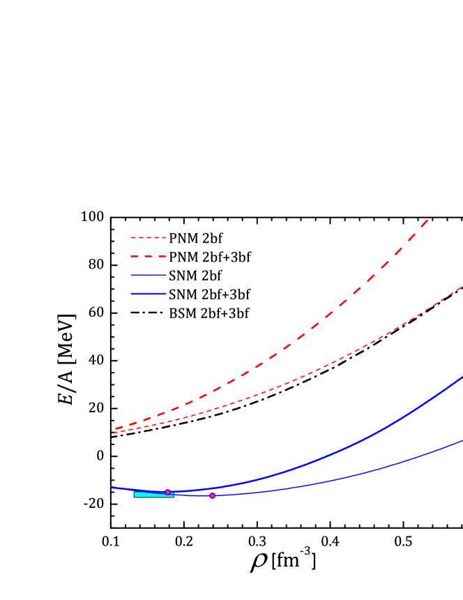
Figure 1: (color online) Energy per nucleon in dense matter as function of baryon density for three states of nuclear matter – symmetric nuclear matter (SNM, solid lines), pure neutron matter (PNM, dashed lines), and beta-stable nuclear matter (BSM, dash-dotted lines). Thick lines are calculated including two-body and three-body nucleon interaction, while thin lines are obtained using two-body forces alone. Circles show positions of the saturation points on the SNM curves; the experimental position of the saturation point is given by filled rectangle.

The proton fraction in the beta-stable nuclear matter can be obtained utilizing the quadratic approximation for the energy per nucleon

$$E=E_{0}+S_{b}(1-2x_{p})^{2}.$$ (35)

This approximation is known to be very accurate up to $x_{p}=0$. Proton fraction resulting from our calculations is shown in Fig. 2 with solid line. The dashed line in the same figure correspond to the proton fraction obtained with two-body forces only. It is seen that inclusion of three-body forces increases the proton fraction. In what follows in all calculations (including those which are referred as “two-body alone”) we always use $x_{p}$ obtained with both two-body and three-body forces. The energy per nucleon corresponding to this proton fraction is shown in Fig. 1 with dash-dotted curve.

Figure 2: (color online) Proton fraction in beta-stable nuclear matter as function of baryon density. Dashed line shows results obtained with two-body forces only.

The effective masses at the Fermi surface are calculated in accordance with Eq. (22). It turns out that the numerical differentiation of the single particle potential produces some fluctuations in the dependence of the effective masses with density. We thus interpolated the numerical values by smooth functions of density within 2% accuracy. The values obtained in this way are shown in Fig. 3. The neutron effective masses as a function of density for beta-stable, symmetric, and pure neutron matter are shown with solid, short dashed, and dot-dashed lines, respectively. Dashed lines show the proton effective mass in the beta-stable nuclear matter. Thin lines correspond to the results obtained with two-body interaction alone. We see, that the medium effects generally decrease the effective masses from the bare value, but inclusion of the three-body forces significantly increase the effective masses with respect to the two-body level. Different results were obtained by Zhang et al. Zhang et al. (2007, 2010) who included an additional rearrangement contribution to the effective mass. The authors report that this term, resulting mainly from the strong density-dependence of the effective three-body force $V^{(3)}_{\rm NN}$, leads to significant decrease of the effective masses. In what follows we do not include the rearrangement contribution, see discussion in Secs. III.1 and IV.3.

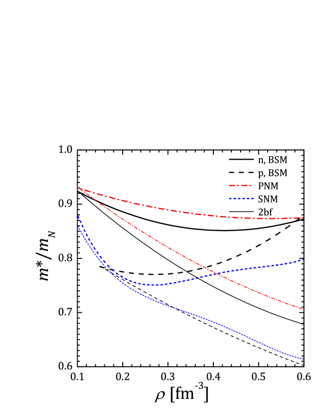
Figure 3: (color online) Effective masses at Fermi surfaces for three states of nuclear matter. Thin lines are obtained with two-body forces alone, while thick lines are calculated including two-body and three-body contributions. Solid, short dashed, and dot-dashed lines show $m^{*}_{n}$ in BSM, SNM, and PNM, respectively, while longer dashed lines show $m_{p}^{*}$ in BSM.

Now we turn to the in-medium cross-sections calculated in accordance with Eqs. (31) and (34). The cross-sections are parameterized by the quantity $E_{\rm c.m.}\equiv p^{2}/m_{N}$ which would be the c.m. energy in the free-space. As an example we selected one density value $\rho=0.35$ fm^-3, approximately twice the nuclear saturation density.

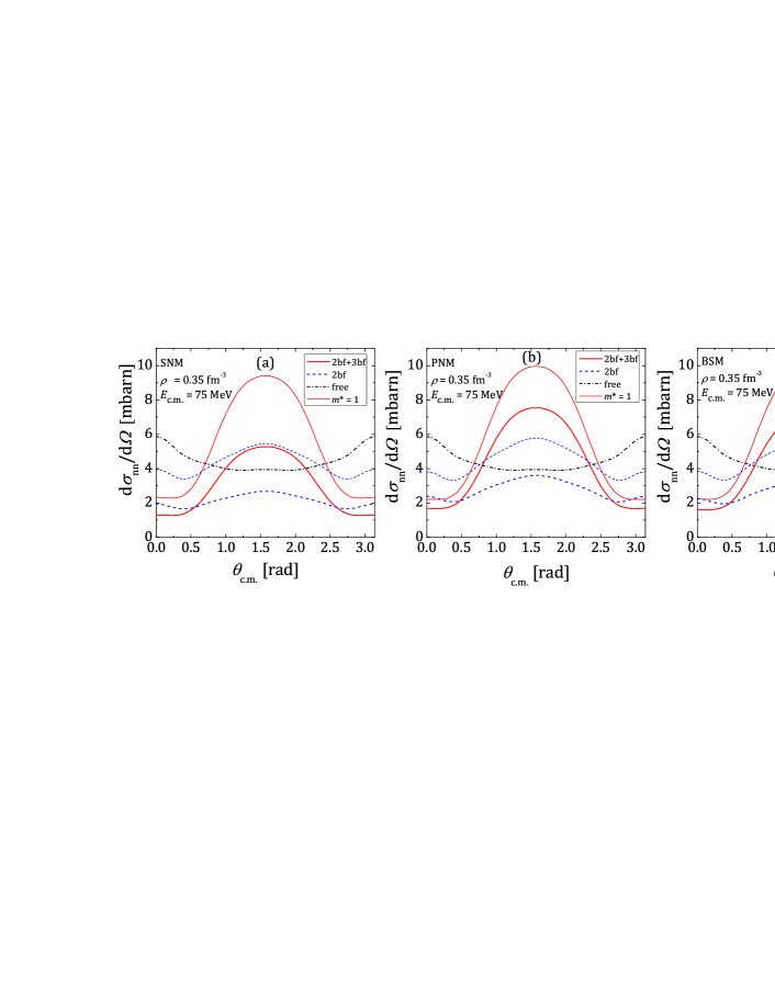
Figure 4: (color online) Differential neutron-neutron cross-section as a function of the c.m. angle at density $\rho=0.35$ fm^-3 and c.m. energy $E_{\rm c.m.}=75$ MeV in symmetric nuclear matter (panel (a)), pure neutron matter (panel (b)), and beta-stable nuclear matter (panel (c)). Dash-dotted lines show the free-space cross-sections. Solid lines are calculated with two-body and three body interactions, dashed lines show the results of calculations with two-body potential only. Thin lines correspond to $m^{*}=1$ case.

In the Figure 4 we show neutron-neutron differential cross-section as a function of the c.m. scattering angle. Three panels (a), (b), and (c) correspond to three considered states of the nuclear matter – symmetric nuclear matter, pure neutron matter, and beta-stable nuclear matter, respectively. In each panel the free-space cross-section is shown by dot-dashed line. Thick dashed lines show the cross-sections obtained with the two-body potential only. These cross-sections are smaller than the free-ones. The in-medium suppression is higher in symmetric nuclear matter than in pure neutron matter and beta-stable neutron matter. By the thin lines in Fig. 4 the cross-sections obtained from Eq. (31) are shown but with bare nucleon mass used in place of the effective mass. Comparison between thin and thick lines shows that it is the effective mass that is responsible for the suppression of the cross-section. The situation changes when three-body forces are included (solid curves in Fig. 4). The inclusion of the three-body forces increases the cross-sections from the two-body level. It becomes comparable to and even higher than the free-space cross-section. The situation is qualitatively similar for the neutron-proton cross-section. The latter is shown in Fig. 5 for symmetric nuclear matter and beta-stable nuclear matter in panels (a) and (b), respectively. Trivially, there is no np cross-section in pure neutron matter.

Zhang et al. Zhang et al. (2007, 2010), in contrast, found that inclusion of three-body forces decreases the in-medium cross-section from the two-body level. There are two main reasons for this. First, the three-body force used by the authors of Refs. Zhang et al. (2007, 2010) differs from ours. We have checked that the inclusion of the three-body force of that type indeed decrease the cross-section. However, the three-body force model used in Zhang et al. (2007, 2010) faces some difficulties in reproducing the saturation point Li et al. (2008, 2006). The second reason is in different approaches to the effective masses. The strong rearrangement decrease of the effective masses leads to corresponding decrease of the in-medium cross-sections.

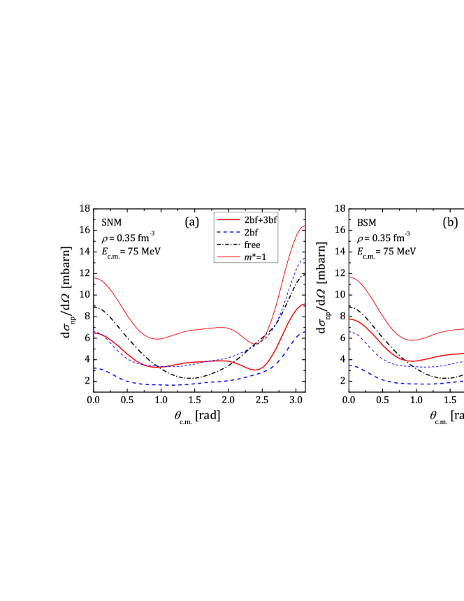
Figure 5: (color online) Differential neutron-proton cross-section as a function of the c.m. scattering angle at density $\rho=0.35$ fm^-3 and c.m. energy $E_{\rm c.m.}=75$ MeV in symmetric nuclear matter (panel (a)) and beta-stable nuclear matter (panel (b)). Notations are same as in Fig. 4.

In the Figure 6 we compare the in-medium cross-sections in the matter with different nuclear asymmetry. Neutron-neutron cross-sections are shown in the (a) panel, and neutron-proton ones in (b) panel. Double dot-dashed lines show free-space cross-sections. Dot-dashed, dashed, and solid lines are for PNM, SNM, and BSM, respectively. Thin lines show the two-body results. We see, that the in-medium nn cross-sections in pure neutron matter and beta-stable neutron matter are close. The reason for that is the small proton fraction $x_{p}$. However, this does not necessary mean that the kinetic coefficients in the PNM and beta-stable matter will be close, see below.

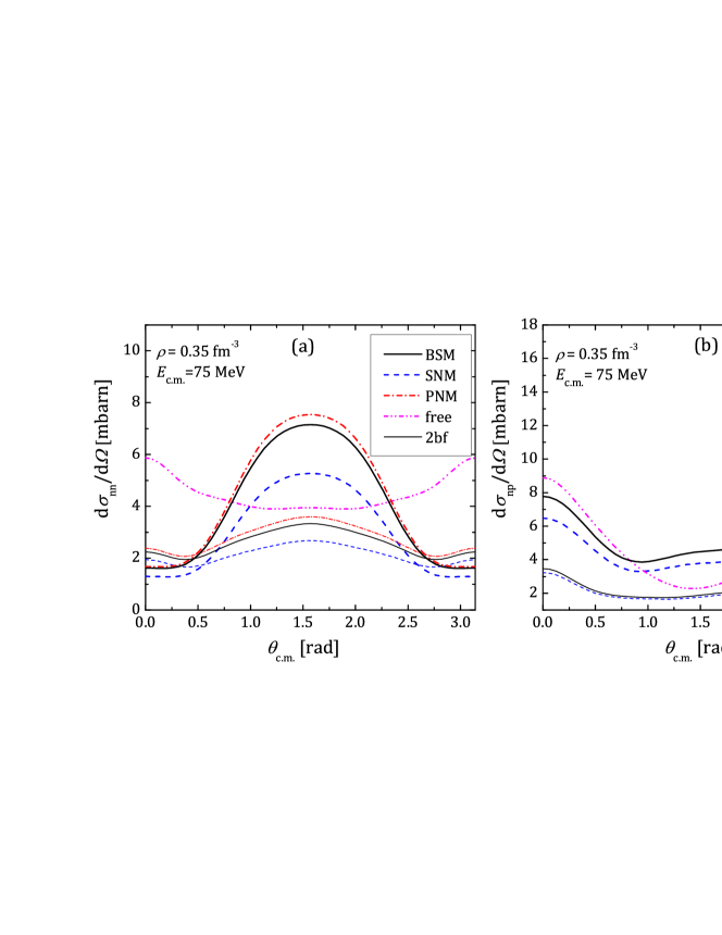
Figure 6: (color online) Differential neutron-neutron (panel (a)) and neutron-proton (panel (b)) cross-sections as a function of the c.m. scattering angle at density $\rho=0.35$ fm^-3 and c.m. energy $E_{\rm c.m.}=75$ MeV in different states. Dot-dot-dashed lines show the free-space cross-section. Solid lines correspond to beta-stable nuclear matter, dashed lines to symmetric nuclear matter, and dot-dashed lines to pure neutron matter. Thin lines show the results obtained with two-body potential alone.

Finally in the Fig. 7 we plot the total neutron-neutron (panel (a)) and neutron-proton (panel (b)) cross-sections, calculated in accordance with Eq. (34). Line styles are the same as in Fig. 6. Both neutron-neutron and neutron-proton cross-sections are suppressed by in-medium effects at smaller values of $E_{\rm c.m.}$ (or, equivalently, c.m. momentum $p$) and become higher than the free-space cross-sections at higher values of energy. Note that the neutron-proton total cross-section in the Fig. 7 (b) have sense only for the symmetric nuclear matter, remind the discussion in Sec. III.3.

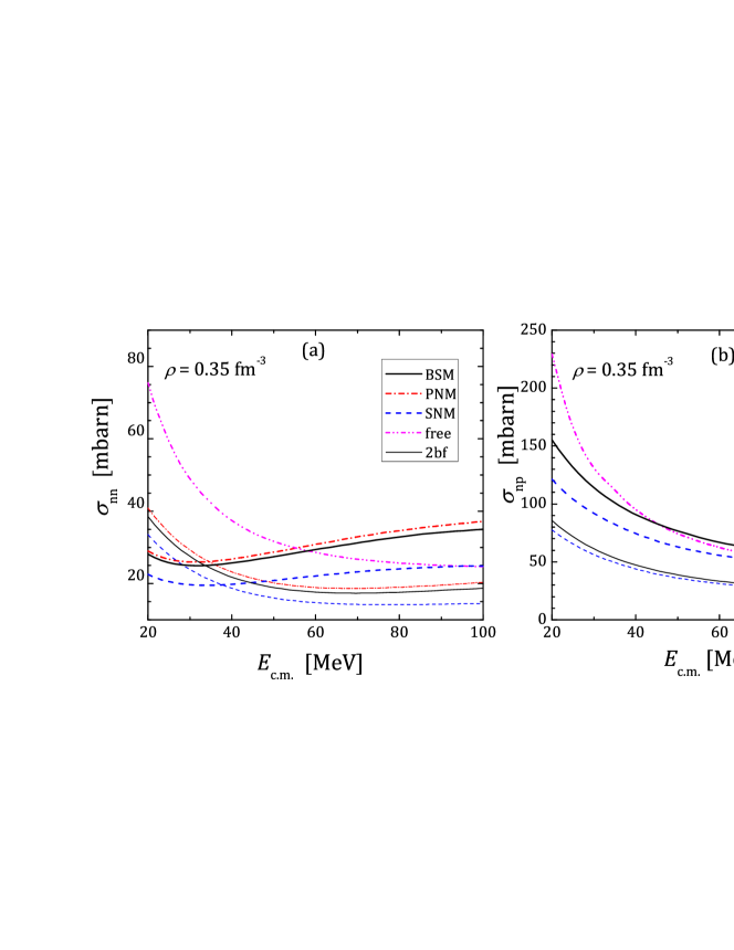
Figure 7: (color online) Total neutron-neutron (panel (a)) and neutron-proton (panel (b)) cross-sections at density $\rho=0.35$ fm^-3 as a function of c.m. energy $E_{\rm c.m.}$ in different states. Notations are the same as in Fig. 6

IV.2 Transport coefficients

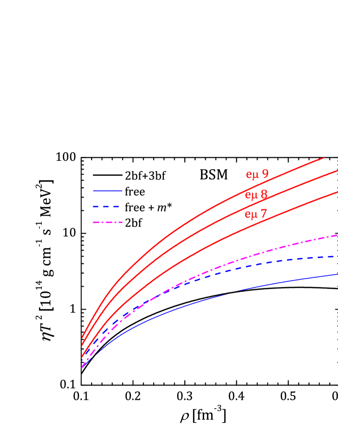
Figure 8: (color online) Shear viscosity of neutrons versus density in beta-stable nuclear matter. Solid line is calculated including all effects discussed in the text. Dash-dotted line represent contribution of two-body forces alone. Thin solid line shows the free-space result, while dashed line is for free space matrix elements, with inclusion of in-medium effective masses. Lines marked e$\mu$ show electron and muon contribution for three values of temperature $T=10^{7}$, $10^{8}$, and $10^{9}$ K (logarithm of temperature is noted near the curves).

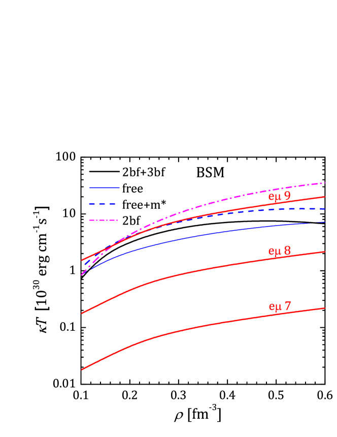
Figure 9: (color online) Thermal conductivity of neutrons versus density in beta-stable nuclear matter. Notations are the same as in Fig. 8.

Figures 8 and 9 show the neutron shear viscosity and thermal conductivity, respectively, in the beta-stable nuclear matter. Both quantities are given by temperature-independent combinations $\eta T^{2}$ and $\kappa T$. The results of full calculations, including two-body and three-body forces are shown by solid lines. Note that here the exact solutions of corresponding systems of kinetic equations are presented. The results obtained neglecting three-body contribution are given by dash-dotted lines in Figures 8 and 9, and the results of free-space calculations are given by thin solid lines. Behavior of both shear viscosity and thermal conductivity is similar. We find that in-medium effects on two-body level increase the kinetic coefficients, while inclusion of UIX three-body force works in opposite direction, decreasing the values back close to the free-space results. To track the effect of effective mass we also plot in Figs. 8 and  9 results of calculations with in-medium effective masses, but free-space scattering matrix elements. These curves go considerably higher than the results of full calculations. Therefore, the in-medium effects on the scattering matrix are as important as the effects of effective mass. In addition, in Figs. 8 and 9 we plot the electron and muon shear viscosity $\eta_{e\mu}$ and $\kappa_{e\mu}$, respectively, in accordance with Refs. Shternin and Yakovlev (2007, 2008b). These quantities has non-standard temperature dependence ($\eta_{e\mu}\propto T^{-5/3}$, $\kappa_{e\mu}\propto T^{-1}$ in the leading order), therefore combinations $\eta_{e\mu}T^{2}$ and $\kappa_{e\mu}T$ are no longer temperature independent Shternin and Yakovlev (2007, 2008b). We consider three values of temperature $T=10^{7}$, $10^{8}$, and $10^{9}$ K, where the $\log_{10}T$ [K] is shown near the corresponding curves. We see that neutron shear viscosity in our model is much smaller than electron and muon one for all densities and temperatures of consideration. This is due to suppression effect of three-body forces. Our result contradicts the results of other authors Benhar and Valli (2007); Zhang et al. (2010); Benhar et al. (2010). This issue will be discussed separately below. For the thermal conductivity, situation is opposite. The relation $\kappa_{n}\gg\kappa_{e\mu}$ is valid for all temperatures, except for the highest $T\sim 10^{9}$ K where neutron and electron-muon contributions become comparable.

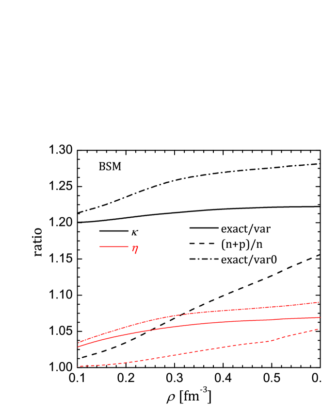
Figure 10: (color online) Ratio between exact and variational values of the kinetic coefficients (solid lines). Thick lines are for thermal conductivity, while thin lines are for shear viscosity. Dashed lines show the relative contribution of protons. Dash-dotted lines give the ratio between the exact values and those obtained in variational approximation with only neutrons as carriers.

In Fig. 8 and 9 the results of the exact solution of the $2\times 2$ system of kinetic equations for neutron-proton subsystem are presented. It is instructive to compare the exact solution to simpler variational calculations which solve simpler algebraic system (8). This is done in Fig. 10 where the ratio between exact and variational solutions is given by thick solid line for $\kappa$ and thin solid line for $\eta$, respectively. We see, that it is enough to employ simple variational expressions with correction factor $C_{\kappa}=1.2$ and $C_{\eta}=1.05$. In the same figure with dash-dotted lines we compare the exact result with variational approximation in which protons are only considered as scatterers. In this case $2\times 2$ system (8) reduces to one equation for the neutron effective relaxation time. In this case the correction coefficients are higher. Finally, we investigate the proton contribution to the kinetic coefficients by plotting the ratios $(\eta_{n}+\eta_{p})/\eta_{n}$ and $(\kappa_{n}+\kappa_{p})/\kappa_{n}$ with thin and thick dashed lines, respectively. It is clear that the proton contribution to shear viscosity can always be neglected. For the thermal conductivity the proton contribution can reach 15% at highest considered density and can be included in the calculations.

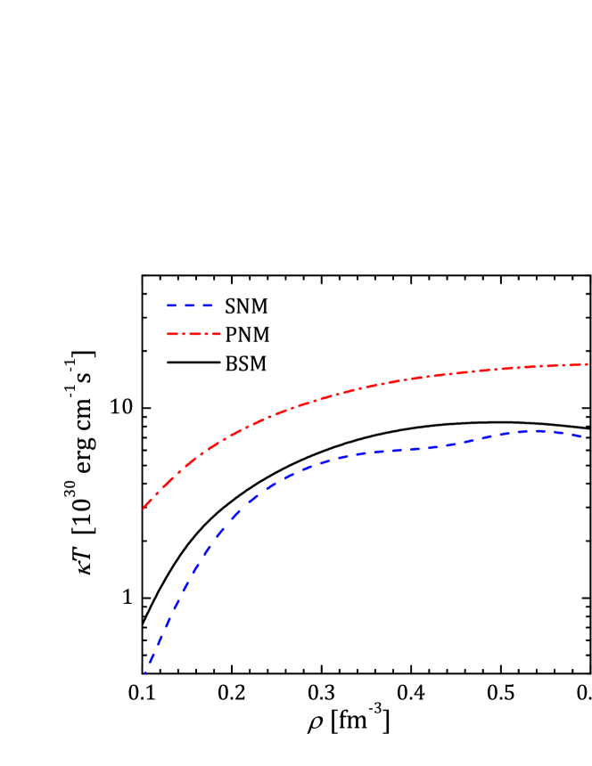
Figure 11: (color online) Total thermal conductivity ($\kappa_{n}+\kappa_{p}$) as a function of density for pure neutron matter (dash-dotted curves), symmetric nucleon matter (dashed curves), and beta-stable nucleon matter (solid curves).

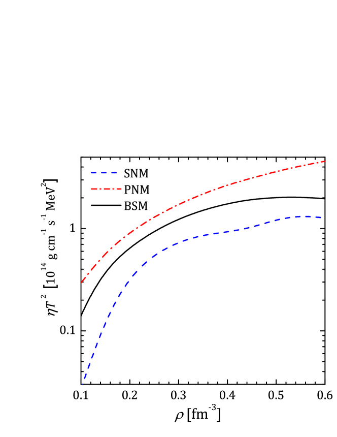
Figure 12: (color online) Total shear viscosity ($\eta_{n}+\eta_{p}$) as a function of density for pure neutron matter (dash-dotted curves), symmetric nucleon matter (dashed curves), and beta-stable nucleon matter (solid curves).

Finally, in Figs. 11 and 12 total thermal conductivity $\kappa_{n}+\kappa_{p}$ and shear viscosity $\eta_{n}+\eta_{p}$, respectively, are plotted for three states of matter – pure neutron matter, symmetric neutron matter, and beta-stable neutron matter. We see that even a small amount of protons (as happens in beta-stable matter, see Fig. 2) leads to considerable reduction of kinetic coefficients. This effect is more pronounced for the thermal conductivity (Fig. 11). It means that the neutron-neutron collision frequencies and neutron-proton collision frequencies are comparable despite low proton fraction. The reason for that lies in the different kinematical restrictions for neutron-neutron and neutron-proton collisions, as well as in the different behavior of neutron-neutron and neutron-proton cross-sections Baiko et al. (2001). Indeed, at small fraction of protons $p_{\rm Fp}\ll p_{\rm Fn}$ and neutron-proton scattering occurs at small c.m. angles ($q<q_{m}(P\approx p_{\rm Fn})\ll p$, see Eq. (13) and Eq. (15)). In this case forward-scattering part of the np cross-section plays the major role. In contrast, the neutron-neutron collisions occur in whole range of c.m. angles ($q<q_{m}(P)=2p$ in Eqs. (12) and (14)). In this case effective collision frequencies are determined mainly by the nn cross-section at large angles. Let us remind, that due to inclusion of $T_{z}=0$ isospin channel, the np cross-section is larger than the nn one. In addition, np cross-section at small scattering angles is considerably increased in comparison to that at large angles. Finally, smaller values of energy give main contribution to the np scattering in comparison with energies relevant for the nn scattering, which additionally increases the contribution from the np scattering.

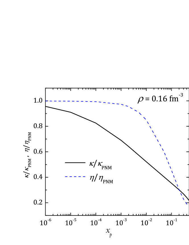
Figure 13: (color online) Ratios $\kappa/\kappa_{\rm PNM}$ (solid lines) and $\eta/\eta_{\rm PNM}$ (dashed lines) of kinetic coefficients in nucleon matter to corresponding quantities in pure neutron matter as a function of proton fraction $x_{p}$ at density $\rho=0.16$ fm^-3. Free-space scattering probabilities and bare masses are used.

We illustrate the importance of the neutron-proton scattering by plotting in Fig. 13 ratios $\kappa/\kappa_{\rm PNM}$ and $\eta/\eta_{\rm PNM}$ of total neutron and proton thermal conductivity and shear viscosity to the same quantities, calculated for the pure neutron matter, as a function of the proton fraction $x_{p}$ at the baryon density $\rho=0.16$ fm^-3. For simplicity, in Fig. 13 we used in-vacuum scattering probabilities and effective masses. One can indeed observe, that for very small proton fractions neutron-proton scattering still contribute significantly to the thermal conductivity. For the shear viscosity this effect is weakened due to additional factor $q^{2}$ in expressions for effective collision frequencies (compare Eq. (15) and Eq. (13)). In both cases, at $x_{p}>0.1$ the use of kinetic coefficients of pure neutron matter as an estimate of true values can lead to an error by a factor more than 2.

IV.3 Comparison with results of other authors

Let us compare our results with the most recent calculations by Zhang et al. Zhang et al. (2010) and Benhar et al. Benhar and Valli (2007); Benhar et al. (2010); Carbone and Benhar (2011).

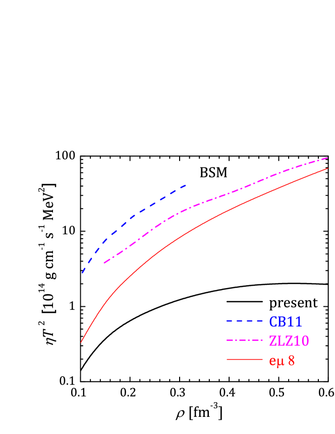
Figure 14: (color online) Comparison of the shear viscosity in beta-stable nuclear matter obtained by different groups. Solid line – present calculations, dashed line – calculations by Carbone and Benhar Carbone and Benhar (2011), dash-dotted line – those by Zhang et al. Zhang et al. (2010). Thin solid line shows electron and muon shear viscosity at $T=10^{8}$ K.

Figure 14 shows the shear viscosity $\eta T^{2}$ for the beta-stable nuclear matter as presented by these groups in comparison with the present work (solid line). The results from Ref. Carbone and Benhar (2011) are given by dashed line and results from Ref. Zhang et al. (2010) by dash-dotted line. For comparison $\eta_{\rm e\mu}T^{2}$ is shown for $T=10^{8}$ K. Apart from the fact that all authors use different equation of state and therefore different proton fractions, and the methods of calculation are different the results in Fig. 14 disagree with each other. The similar situation is observed in case of the thermal conductivity as shown in Fig. 15.

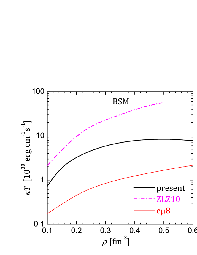
Figure 15: (color online) Comparison of the thermal conductivity in beta-stable nuclear matter obtained by different groups. Notations are same as in Figure 14.

Unfortunately, the calculations of Benhar et al. for the thermal conductivity in beta-stable nuclear matter are not available. However, Zhang et al. Zhang et al. (2010) results (dot-dashed curve in Fig. 15) lie much higher than the present calculations.

In attempt to find the source of this huge discrepancy we analyzed in detail the models used in the series of papers Benhar and Valli (2007); Benhar et al. (2010); Carbone and Benhar (2011) and Zhang et al. (2010, 2007). To begin with we consider the simpler case of pure neutron matter. In this case it is possible to construct the approximate expressions for the shear viscosity and thermal conductivity which depend only on the total neutron-neutron cross-section at the c.m. energy on the Fermi surface $E_{\rm c.m.}=p_{\rm Fn}^{2}/m_{N}$, see Appendix B for details. It is important, that these approximate expressions provide an independent test of the calculations for the free-scattering case, where the in-vacuum cross-section is used. As the total in-vacuum nn cross-section is known relatively well, the “free” result of any calculation must lie close to the values obtained from the approximate expressions. The results of our calculations, as well as those in Refs. Baiko and Haensel (1999); Baiko et al. (2001), satisfy this criterion. Zhang et al. Zhang et al. (2010) present both shear viscosity and thermal conductivity in PNM free case, while Benhar et al. Benhar and Valli (2007); Benhar et al. (2010) show only the shear viscosity for the free case. The results of both groups, at the first glance, strongly disagree with the results presented here, and do not agree with the approximate expression (see Fig. 16 and 17). The careful examination of the expressions in Refs. Zhang et al. (2010); Benhar and Valli (2007); Benhar et al. (2010) shows that in the free case the authors still incorporate some in-medium effects through the Fermi velocities in the definitions of the kinetic coefficients in eqs. (2) and (3) in Ref. Zhang et al. (2010), eq. (1) in Ref. Benhar and Valli (2007), eq. (24) in Ref. Benhar et al. (2010). The factor $v_{F}^{2}$ leads to the appearance of squared effective mass in the expressions for the kinetic coefficients. In addition, eqs. (2)–(6) of Benhar and Valli Benhar and Valli (2007) indicate that these authors lost the factor $\pi$ in the expression for the averaged scattering probability, remind the remark in the end of the Sec. II and Eq. (43). Therefore their result and the results of the subsequent papers Benhar et al. (2010); Carbone and Benhar (2011) are overestimated by the factor of $\pi$. Therefore we corrected the results of Ref. Zhang et al. (2010) by the factor $m_{n}^{*2}$, where neutron effective mass is taken from the fig. 2 in Zhang et al. (2010) and the result of Benhar and Valli (2007) for viscosity by the factor $m_{n}^{*2}/\pi$. The latter effective mass is not available from the references and we assumed $m_{n}^{*}\approx 0.8m_{N}$. This value is consistent with the dot-dashed curve in fig 1(a) in Ref. Benhar and Valli (2007) which is reported to be obtained from eqs. (43) and (46) of Ref. Baiko and Haensel (1999) with the same effective mass as used elsewhere. Note, that expressions in Ref. Baiko and Haensel (1999) contain the fourth power of $m_{n}^{*}$ as those authors used the in-vacuum transition probability, while authors of Ref. Benhar and Valli (2007) use the in-vacuum cross-section (their eq. (6)). The discrepancy between the results of Benhar and Valli Benhar and Valli (2007) and Baiko and Haensel Baiko and Haensel (1999) for the “free scattering” approximations is due to the different effective mass power and the $\pi$ factor, not due to the correction factor to the variational solution as were incorrectly assumed by authors of Ref. Benhar and Valli (2007). In fact, this correction, although small for the shear viscosity, is included in eqs. (43) and (46) in Ref. Baiko and Haensel (1999).

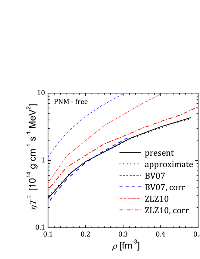
Figure 16: (color online) Comparison of the shear viscosity in PNM in free scattering approximation as reported by different groups. Solid line shows the results of the present calculations, dotted line correspond to the approximate expression. Thin dashed and dash-dotted lines show the results of Ref. Benhar and Valli (2007) and Ref. Zhang et al. (2010), respectively. Thick lines of the corresponding type show the corrected results, see text for details.

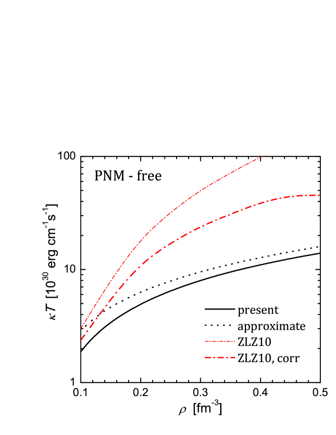
Figure 17: (color online) Comparison of the thermal conductivity in PNM in free scattering approximation as reported by different groups. Notations are the same as in Fig. 16.

The “corrected” values of shear viscosities are shown in Fig. 16 with thick dashed line for Benhar and Valli calculations and with thick dash-dotted line for Zhang et al. calculations. The uncorrected values are shown with thin lines. The results of the present paper are shown with the solid line, while the approximate result is shown by the dotted line and nearly coincides with the exact result. Note that we multiplied the approximate variational expression by the correction factor 1.05. One observes, that the results of Benhar and Valli agree well with the approximate expression, while Zhang et al. curve has qualitatively the same behavior, but gives somewhat higher values. The different situation is observed for the thermal conductivity, as shown in Fig. 17. Again by the solid and dotted lines we show the result of the present and approximate calculations. Now the approximate expression (which is corrected by the factor 1.2) is less accurate than in the case of the shear viscosity. Nevertheless the results of Zhang et al. Zhang et al. (2010), corrected by the $m_{n}^{*2}$ factor, still go much higher. In order to check if this can be the result of the different model used, let us look at the cross-sections reported in Refs. Zhang et al. (2010, 2007). In Ref. Zhang et al. (2007) the Argonne v14 potential was used, while in Ref. Zhang et al. (2010) authors used Bonn-B potential. The reported cross-sections are close, as expected. However, one can note that the nn cross-sections (for the free scattering) in Ref. Zhang et al. (2010, 2007) are different from those obtained in the present paper. One difference is that these authors clearly plot 1/2 of the differential $nn$ cross-sections, so that the c.m. solid angle would be 4$\pi$. Another difference is that the cross-sections have much stronger dependence on $\theta_{\rm c.m.}$ at forward and backward scattering than those obtained here, or in other works (for instance, Li and Machleidt (1994); Fuchs et al. (2001)). Although the reason for this difference is unknown to us, we found that we can reproduce well the free-space nn cross-sections in Refs. Zhang et al. (2010) and Zhang et al. (2007) (for the corresponding potentials) if we omit the phase factor $i^{\ell^{\prime}-\ell+\bar{\ell}-\bar{\ell}^{\prime}}$ in Eq. (29). This factor comes from the partial wave expansion of the plane waves. This affects only non-diagonal elements, therefore the total cross-section does not change if this phase factor is omitted. Hence the resulting kinetic coefficients still should be close to the approximate expressions. We checked this explicitly, using the cross-sections calculated without the phase factor. This test allows to check the results of Zhang et al. (2010) irrespectively if the phase factor omission is a real reason for such form of the cross-section, or where it is a coincidence. We found that the both shear viscosity and thermal conductivity are still in agreement with the corresponding approximate expressions, and did not found anything similar to the plot in Fig. 17. Therefore we conclude, that the thermal conductivity calculations in Ref. Zhang et al. (2010) are incorrect and probably give overestimated values for this kinetic coefficient, while the shear viscosity calculations of Ref. Zhang et al. (2010) and Refs. Benhar and Valli (2007); Benhar et al. (2010) (if divided by $\pi$) look plausible.

Now let us return to the shear viscosity in Fig. 14. Results of the in-medium calculations by Zhang et al. Zhang et al. (2010) and Carbone and Benhar Carbone and Benhar (2011), even corrected by $\pi$, are much higher than our calculations. These groups used different approaches, and we discuss them separately.

Zhang et al. Zhang et al. (2010) reports approximately order of magnitude increase of the shear viscosity due to the medium effects. The above analysis of their in-vacuum results (Fig. 16) suggests that in both “free” and “in-medium” calculations same Fermi velocities were used. Therefore the increase in the in-medium viscosity is solely due to the decrease in the in-medium cross-section. However, as follows from the plots in Refs. Zhang et al. (2010) and Zhang et al. (2007) this decrease is lower, at most by the factor of 2-3 in the high-energy region of interest. Hence the increase in the shear viscosity if calculated properly should be of the same order. Note that for shear viscosity in PNM and SNM as well as for thermal conductivity in all three states this increase is indeed reported to be 2-4 in Ref. Zhang et al. (2010). Therefore we believe that the in-medium shear viscosity for BSM in Ref. Zhang et al. (2010) is calculated inaccurately and is overestimated by a factor of 3-5. The remaining difference between our shear viscosity and one by Zhang et al. Zhang et al. (2010) would be still about a factor of 3-5, but the latter difference is due to the different physical model used. Indeed, as already stated before, they used different model for three-body force, which led to the decrease of in-medium cross-section, while the three-body force we employ operates in opposite directions. The second source of difference is the rearrangement modifications of the effective masses. The inclusion of the rearrangement led Zhang et al. Zhang et al. (2010, 2007) to a strong reduction of the effective masses, while in contrast we observe the increase of effective masses due to three-body forces (see Fig. 3). These factors again work in the opposite directions. Nevertheless, the use of the modified effective mass is cautioning. Indeed, the origin of the rearrangement contribution lies in the functional dependence of the $G$-matrix on the occupation numbers. This leads to difference between Landau quasiparticle energy $\epsilon_{L}(p)$ given by the functional derivative of the total energy of the system with respect to the distribution function and the Brueckner self-consistent single-particle potential $\epsilon(p)$ in Eq. (20). The two quantities would coincide provided that the functional derivative acting on the $G$-matrix is neglected. Therefore the quasiparticle effective mass which is found from $\epsilon_{L}(p)$ deviates from the Brueckner effective mass $m^{*}$. Physically, including rearrangement corrections incorporates to some extent the effects of the medium polarization. However, for consistency, the same effects should be included in the quasiparticle interaction. Therefore this interaction (and quasiparticle scattering amplitude as well) must differ from the Brueckner $G$-matrix at the same footing. Provided strong modification of the effective mass one could expect strong modification of the quasiparticle scattering amplitude at the same level of approximation. The size and the direction (increase or decrease) of this effect is unknown and requires a separate consideration, which lies outside the scope of the present paper. It is possible that it can suppress the kinetic coefficients more, or, in opposite, there is a possibility of counter-compensation of the effective mass effect.

In a series of papers Benhar and Valli (2007); Benhar et al. (2010); Carbone and Benhar (2011) the correlated basis function (CBF) formalism was used which is different from the BHF approach. However, in Ref. Benhar et al. (2010) authors compared results obtained in CBF and $G$-matrix approaches and obtained overall agreement. The reasons of the huge in-medium increase of kinetic coefficients in these works are different than in Zhang et al. Zhang et al. (2010). First of all, we note that the three-body force effects are reported to be small. In fact, the comparison of the results in fig. 1.(b) in Ref. Benhar and Valli (2007) and in fig. 5 in Ref. Benhar et al. (2010) where the three-body forces, as written, are not included, shows that the three-body forces even slightly decrease the shear viscosity. Therefore the strong in-medium increase of the shear viscosity (again $\sim 10$) is due to the squared effective mass, which gives a factor of 2, and due to decrease of the cross-section, which is a factor of 5, according to fig. 4 in Ref. Benhar et al. (2010) (note that the free-space cross-section reported in the same figure is underestimated by the factor $\sim$1.5 with respect to the true values). Let us note, that we do not observe so strong decrease of the in-medium cross-section at the two-body level (Fig. 7). Same smaller decrease (factor of 2) is also found by the other authors (e.g. Li and Machleidt (1994); Fuchs et al. (2001)), including Zhang et al. Zhang et al. (2007). In addition, the proton fraction used by Carbone and Benhar Carbone and Benhar (2011) is slightly lower than one we use.

Finally, we stress that inaccuracies in the recent calculations of the two groups do not allow one to deduce which percentage of the effect is due to the selection of the physical model and which part is related to these inaccuracies.

V Conclusions

We have calculated thermal conductivity and shear viscosity of nuclear matter in beta-equilibrium. The neutron and proton interaction was described by the Argonne v18 potential with inclusion of effective Urbana IX three-body forces. The scattering of particles were treated in the non-relativistic Brueckner-Hartree-Fock approximation with the continuous choice of the single-particle potential.

Our main results are as follows

1. Shear viscosity and thermal conductivity of nuclear matter are modified by the medium effects in comparison with the values obtained from the free-space cross-sections. However this modification is not so strong as reported previously.

2. The medium effects of the renormalization of the squared matrix element due to the Pauli blocking in the intermediate states and of the effective mass via the reduction of the density of states are comparable and cannot be separated.

3. The Urbana IX three-body forces lead to the increase of the scattering probabilities and, therefore, to a considerable reduction of the kinetic coefficients in comparison to the two-body case. The effect of the three-body forces is sizable at $\rho\gtrsim 0.15$ fm^-3.

The question remains how the kinetic coefficients would depend on the particular model for the three-body force. It is clear that they are more sensitive to change of the model than the equation of state. The results of Ref. Zhang et al. (2010) suggest that the inclusion of different three-body forces could lead to increasing of the kinetic coefficients in contrast to the results of the present paper. The investigation of the model-dependence of the values of the kinetic coefficients is a good project for the future.

In all our calculations we used the non-relativistic BHF framework. The non-relativistic approach could be questioned, especially at high density. However it has been shown Brown et al. (1987) that the main relativistic effect, as included in the Dirac-Bruckner (DBHF) scheme, is equivalent to the introduction of a particular three-body force at the non-relativistic level. Therefore the use of a TBF in BHF calculations incorporates in an effective way the relativistic corrections.

Finally let us note, that we have neglected the possible effects of superfluidity. It is believed that the neutrons and protons in the neutron star cores can be in the superfluid state. The critical temperatures of the superfluid transition are very model-dependent and can vary as $T_{c}\sim(10^{8}-10^{10})$ K (see, for example, Lombardo and Schulze (2001)). The effects of superfluidity on the kinetic coefficients were considered in the approximate way in Refs. Baiko et al. (2001); Shternin and Yakovlev (2008b). The investigation of these effects is outside the scope of the present paper.

Appendix A Angular integrations

We deal with the integrals of the form

$${\cal Q}^{(ij)}=\int\limits_{|p_{\rm Fc}-p_{\rm Fi}|}^{p_{\rm Fc}+p_{\rm Fi}}{\rm d}P\int\limits_{0}^{q_{m}(P)}{\cal Q}(P,q)\frac{P^{i}q^{j}\,{\rm d}q}{\sqrt{q_{m}^{2}-q^{2}}},$$ (36)

where ${\cal Q}(P,q)$ is expanded in the Legendre polynomials

$${\cal Q}(P,q)=\sum_{L}{\cal Q}_{L}(P){\cal P}_{L}\left(1-\frac{q^{2}}{2p^{2}}\right).$$ (37)

Then the internal integral (over $q$) can be obtained analytically

$$\int\limits_{0}^{q_{m}}\frac{q^{j}{\rm d}q}{\sqrt{q_{m}^{2}-q^{2}}}{\cal P}_{L}\left(1-\frac{q^{2}}{2p^{2}}\right)=\frac{q_{m}^{j}}{2}B\left(\frac{j+1}{2},\frac{1}{2}\right){}_{3}F_{2}\left(-L,L+1,\frac{j+1}{2};1,\frac{j}{2}+1;\frac{q_{m}^{2}}{4p^{2}}\right),$$ (38)

where $B\left(\frac{j+1}{2},\frac{1}{2}\right)$ is the beta-function, and ${}_{3}F_{2}$ is the generalized hypergeometric function. The latter function, in fact, reduces to the $L-1$ order polynomial in $q_{m}^{2}/(4p^{2})$, as its first argument, $-L$, is a negative integer.

Appendix B Approximate expressions for neutron kinetic coefficients

The simplest variational expressions for thermal conductivity and shear viscosity of one-component Fermi-liquid read Baym and Pethick (1991)

$$\kappa_{\rm var} = \frac{20\pi^{2}p_{F}^{3}}{9m^{*4}\langle W\rangle}\frac{1}{T}\left(3-\lambda_{\kappa}\right)^{-1},$$ (39)

$$\eta_{\rm var} = \frac{4p_{F}^{5}}{5m^{*4}\langle W\rangle}\frac{1}{(k_{B}T)^{2}}\left(1-\lambda_{\eta}\right)^{-1},$$ (40)

where $\lambda_{\kappa}$ and $\lambda_{\eta}$ encapsulate the kinematical factors, namely

$$\langle W\rangle(1-\lambda_{\kappa})=4\langle W\sin^{2}\frac{\theta}{2}\rangle,$$ (41)

$$\langle W\rangle(1-\lambda_{\eta})=3\langle W\sin^{4}\frac{\theta}{2}\sin^{2}\phi\rangle.$$ (42)

The Abrikosov-Khalatnikov angle $\phi$ in the considered case is equal to the c.m. angle $\theta_{\rm c.m.}$, and angle $\theta$ is connected to the relative momentum as $p=p_{F}\sin(\theta/2)$. The scattering amplitude $W$ is connected to the differential cross-section as

$$W=\pi{\cal Q}=\frac{16\pi^{3}\hbar^{4}}{m^{*2}}\frac{{\rm d}\sigma}{{\rm d}\Omega_{\rm c.m.}}.$$ (43)

The Abrikosov-Khalatnikov averaging is defined as

$$\langle W\rangle=\frac{1}{2\pi}\int_{0}^{\pi}{\rm d}\theta\sin(\theta/2)\int_{0}^{2\pi}{\rm d}\phi\,W(\theta,\phi).$$ (44)

On can observe, that the main contribution to averages (41)–(42) is given by the region of $\theta\approx\pi$ due to powers of $\sin(\theta/2)$ in kinematical factor. Therefore the result will be mainly determined by the cross-section in the high-energy region $p\sim p_{F}$. Assuming also that the angular structure of the cross-section is flat (which is justified for neutron-neutron scattering at the energies of interest) we can substitute

$$\frac{{\rm d}\sigma}{{\rm d}\Omega_{\rm c.m.}}\to\frac{\sigma_{\rm tot}}{2\pi}.$$ (45)

Note that for identical particles the possible scattering solid angle is $2\pi$, not $4\pi$. Under these two approximation, the final expressions are

$$\kappa_{\rm var} \approx \frac{5p_{F}^{3}}{106m^{*2}T}\left[\sigma_{\rm tot}(p=p_{F})\right]^{-1}$$ (46)

$$\eta_{\rm var} \approx \frac{p_{F}^{5}}{16\pi^{2}m^{*2}(k_{B}T)^{2}}\left[\sigma_{\rm tot}(p=p_{F})\right]^{-1}.$$ (47)

For bare particles it is convenient to write $E_{\rm c.m.}=2p_{F}^{2}/m$ in the argument of the total cross-section instead of $p=p_{F}$. Note that the approximations (46)–(47) are good as long as total cross section does not change significantly in the region of large $\theta$. It is easy to write more general expression, assuming only the flat angular dependence. In this case kinetic coefficients would be determined by integration of the total cross-section over the laboratory energy with corresponding kinematical factors.