Search for a stochastic gravitational-wave background using a pair of torsion-bar antennas

Abstract

We have set a new upper limit on the stochastic gravitational-wave background using two prototype torsion-bar antennas (TOBAs). A TOBA is a low-frequency gravitational-wave detector with bar-shaped test masses rotated by the tidal force of gravitational waves. As a result of simultaneous 7-hour observations with TOBAs in Tokyo and Kyoto in Japan, our upper limit with a confidence level of 95% is $\Omega_{\rm gw}h_{0}^{2}<1.9\times 10^{17}$ at 0.035 – 0.830 Hz, where $h_{0}$ is the Hubble constant in units of 100 km/s/Mpc and $\Omega_{\rm gw}$ is the gravitational-wave energy density per logarithmic frequency interval in units of the closure density. We successfully updated the upper limit and extended the explored frequency band.

I Introduction

Detecting a stochastic gravitational-wave background (SGWB) is one of the most ambitious targets in gravitational-wave (GW) astronomy. A SGWB is a superposition of GWs produced in the early Universe and GWs emitted from astronomical sources with amplitudes too small to be resolved. Direct observation of a SGWB is fundamentally important to understanding how the universe evolved because a GW can carry information about the universe before the epoch of the last scattering of the cosmic microwave background (CMB) photons due to its high transparency. Revealing the frequency dependance as well as the amplitude of a SGWB will strongly constrain many inflation models since the phase transition of the vacuum or preheating of the universe will produce peaks in the power spectrum density (PSD) of a SGWB Buchmüller et al. (2013); Nakayama et al. (2008).

Several upper limits on a SGWB have been established by observations. For example, interferometric GW detectors, LIGO and Virgo, have set an upper limit of around 200 Hz Abbott et al. (2009). LIGO and a resonant bar detector ALLEGRO were used together to establish an upper limit of around 900 Hz. Two cryogenic resonant bars Explorer and Nautilus have searched for a SGWB at 900 Hz Astone et al. (1999). Other than those, a pair of synchronous interferometers have placed an upper limit at 100 MHz Akutsu et al. (2008). At lower frequencies, upper limits have been set at $10^{-6}-10^{-3}$ Hz by Doppler tracking of the Cassini spacecraft Armstrong et al. (2003), and at $10^{-9}-10^{-7}$ Hz by pulsar timing that measured the fluctuations in pulse arrival times from PSR B1855+09 Maggiore (2000). COBE set an upper limit at $10^{-18}-10^{-16}$ Hz by observing the CMB Allen (1996). Regarding indirect evidence, the helium-4 abundance resulting from big-bang nucleosynthesis (BBN) Maggiore (2000) and measurement of the CMB and matter power spectra Smith et al. (2006) set a constraint on the integrated cumulative energy density of a SGWB.

In addition to these observations, a torsion-bar antenna (TOBA) has opened the frequency band that other GW detectors cannot access Ando et al. (2010). A TOBA is a GW detector with bar-shaped test masses, which is sensitive at low frequencies such as 0.1 – 1 Hz even on the ground. We have already set the first upper limit at 0.2 Hz of $\Omega_{\rm gw}h_{0}^{2}\leq 8.7\times 10^{17}$ using a 20 cm scaled prototype TOBA Ishidoshiro et al. (2011). However, this upper limit was set using a single detector, and it is difficult to distinguish a SGWB signal from noise using only one detector because the waveform of a SGWB is random and unpredictable. Therefore, simultaneous observations with multiple detectors are required for a direct search for a SGWB. In addition, the signal-to-noise ratio is improved by the square root of the observation time because the uncorrelated noises at two separated places would be suppressed. Therefore, we searched for a SGWB by the cross-correlation analysis with two prototype TOBAs. As a result, we were able to update the upper limit on a SGWB and extend the explored frequency region. We present the search procedure and results in this paper.

II Observation

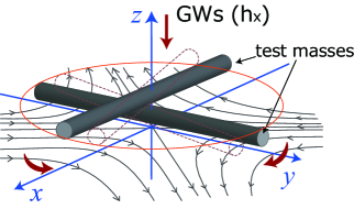
Figure 1: (color online) A conceptual drawing of a TOBA. Two test mass bars are positioned orthogonally and rotate differentially due to the tidal force of the GWs.

A TOBA Ando et al. (2010) is a GW detector composed of two bar-shaped orthogonal test masses that rotate differentially due to the tidal force caused by GWs as shown in Fig. 1. Its angular fluctuation $\theta(t)$ obeys the equation of motion:

$$I\ddot{\theta}(t)+\gamma\dot{\theta}(t)+\kappa\theta(t)=\frac{1}{4}\ddot{h}_{ij}q^{ij},$$ (1)

where $I,\gamma,\kappa,h_{ij}$, and $q^{ij}$ are the moment of inertia, the dissipation term, the spring constant in the rotational degree of freedom, the amplitude of a GW, and the quadropole moment of the test mass, respectively. This results in a simple equation $\tilde{\theta}(f)=q^{ij}h_{ij}/2I$ above the resonant frequency $f_{0}=\sqrt{\kappa/I}/2\pi$. TOBA is fundamentally sensitive at lower frequencies, even on the ground. The low resonant frequency in the rotational degree of freedom $f_{0}$ on the order of a few millihertz makes the test mass free at 0.1 – 1 Hz. The small rotational seismic motion also contributes to the good sensitivity at low frequencies.

We have developed small prototype TOBAs in Tokyo and Kyoto. The longitude and latitude of the two sites are $139.76^{\circ},35.71^{\circ}$ (Tokyo) and $135.78^{\circ},35.03^{\circ}$ (Kyoto). Each prototype TOBA has one 20 cm test mass bar that is magnetically levitated by a pinning effect between a magnet attached at its top and a superconductor at the top of the vacuum tank Ishidoshiro et al. (2010). The angular fluctuation of the test mass is read by a Michelson interferometer; the two laser beams split by a beam splitter hit mirrors attached to both ends of the test mass. Therefore, the difference in the two beam path lengths is proportional to the rotation angle of the test mass. Both test masses are oriented in a north-to-south direction and controlled by coil-magnet actuators so that the fringes of the interferometers are kept in the middle.

We performed simultaneous observations with the prototypes for about 7 hours from 21:21 JST to 4:48 JST on October 29, 2011. Figure 2 shows the equivalent strain noise spectra of the two detectors averaged over the whole observation time. The strains are limited by seismic noise coupled from translational motion at frequencies higher than 0.5 Hz and by the magnetic coupling noise at lower frequencies Ishidoshiro et al. (2011). The noise level is relatively high because there are several glitches which are clearly not a GW signal.

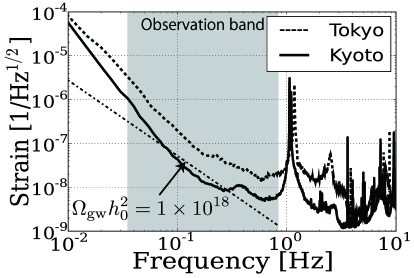
Figure 2: Equivalent strain noise spectra of two detectors. Dashed and solid lines indicate spectra of Tokyo and Kyoto respectively. The sensitivity in the Tokyo data is lower than that in the Kyoto data due to there being many glitches in the data from Tokyo. These glitches were removed during data selection.

III Analysis

The amplitude of a SGWB is usually characterized by the dimensionless quantity $\Omega_{\rm gw}$ defined as

$$\Omega_{\rm gw}=\frac{f}{\rho_{\rm c}}\frac{d\rho_{\rm gw}}{df},$$ (2)

where $\rho_{\rm c}=3c^{2}H_{0}^{2}/8\pi G$ is the critical energy density of the universe and $\rho_{\rm gw}=\langle\dot{h}_{ij}\dot{h}^{ij}\rangle c^{2}/32\pi G$ is the energy density of a SGWB. Then, the PSD of a SGWB can be written as

$$S_{\rm gw}(f)=\frac{3H_{0}^{2}}{10\pi^{2}}f^{-3}\Omega_{\rm gw}(f),$$ (3)

where $H_{0}$ is the Hubble constant. Here we assume that a SGWB is stationary, isotropic, unpolarized and Gaussian, and $\Omega_{\rm gw}={\rm constant}$ in our observation band.

In order to search for a SGWB, we take the general cross correlation between the two detector outputs in strain $s_{1}(t)$ and $s_{2}(t)$:

$$Y = \int_{-T/2}^{T/2}dt\int_{-T/2}^{T/2}dt^{\prime}s_{1}(t)s_{2}(t^{\prime})Q(t-t^{\prime})$$ (4)

$$\sim \int_{-\infty}^{+\infty}df\tilde{s}_{1}^{*}(f)\tilde{Q}(f)\tilde{s}_{2}(f).$$

Here, a tilde notates Fourier transformed functions. $T$ and $\tilde{Q}(f)$ are the observation time and a filter function chosen so that the signal-to-noise ratio of $Y$ is maximized. The expected value of $Y$ depends only on a SGWB since the noise in each detector is uncorrelated. Considering Eq. (3), $\tilde{Q}(f)$ is written as

$$\tilde{Q}(f)=C\frac{\gamma(f)}{P_{1}(f)P_{2}(f)f^{3}},$$ (5)

where $P_{i}(f)$ is the power spectrum density of the $i$th detector’s output, and $C$ is a normalization factor set in order to give $\langle Y\rangle=\Omega_{\rm gw}h_{0}^{2}T$. $h_{0}$ is the normalized Hubble constant defined as $h_{0}=H_{0}/100{\rm km}/{\rm sec}/{\rm Mpc}$. $\gamma(f)$ is the overlap reduction function that represents the difference between the two detector responses. In this case, $\gamma(f)$ is almost unity below 10 Hz since distance between the two sites is about 300 km which is short compared to the GW wavelength and the bars were oriented in the same direction. Please refer to Maggiore (2008) for further details.

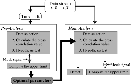
Figure 3: Flowchart of the analysis. The preanalysis and main analysis are similar except that the preanalysis is performed using the time-shifted data to tune the parameters.

A flowchart of the data analysis is shown in Fig. 3. The data stream is divided into $N$ segments with 50% overlap, and fast Fourier transformation was performed using a Hanning window.

After the data are transformed into $\tilde{s}_{iJ}(f)$, the data for the $J$th segments of $i$th detector’s output, we removed segments in which the noise was obviously not a GW signal and was large enough to affect the result. The removed segments were selected according to the band-limited root mean square (rms). We did not use the main observation band for data selection to avoid unintentionally removing a signal. Instead, we calculated the rms below 0.05 Hz and above 1 Hz as an indicator of the data selection in order to remove segments where the magnetic coupling noise or seismic noise was large.

Next, the cross-correlation value $Y/T_{\rm seg}$, which corresponds to $\Omega_{\rm gw}h_{0}^{2}$, is calculated at each surviving segment. Here, $T_{\rm seg}$ is the length of the segments. We limited the integration frequency band to where $\tilde{Q}(f)$ was biggest, since $\tilde{Q}(f)$ is largest at frequencies where the sensitivity to a SGWB is the best.

We then judged that a SGWB signal is present if $\langle Y\rangle/T_{\rm seg}$, where $\langle Y\rangle$ is the average cross-correlation value for the segments, is larger than the detection threshold. This test is based on the Neyman-Pearson criterion Helstrom (1968). A detection threshold depends on the probability distribution of $\langle Y\rangle/T_{\rm seg}$ without a signal and the false alarm rate $\alpha$. The probability distribution, which reflects the background, is estimated from observed data. A histogram of $\langle Y_{JK}\rangle/T_{\rm seg}$, which is the cross correlation between $\tilde{s}_{1J}(f)$ and $\tilde{s}_{2K}(f)(J\neq K,K\pm 1)$, is proportional to the probability distribution without a signal because there is no correlation between two segments whose time differs by more than the time constant of a target signal, even though a signal is present in the original data stream. Note that we did not put the correlation between the segments next to each other so the correlation in overlapped time does not affect the result. Also, the data are considered to be sufficiently stationary through the observation such that the correlation values of the segments with large separation of time will not cause the histogram to differ from the true probability distribution. Thus, the detection threshold $z_{\alpha}$ is set so that the integral of the probability distribution from $z_{\alpha}$ to $\infty$ is equal to $\alpha$. When $\langle Y\rangle/T_{\rm seg}$ calculated with time adjusted data is larger than $z_{\alpha}$, a signal is present. Here, the correlation value is not necessarily positive because we did not align the plus and minus of the signal in this analysis.

If a SGWB signal is not detected, an upper limit is set by mock signal injection based on a Bayesian method. We injected a mock signal into the real data and searched for the mock signal as mentioned above. The mock signal is the random data stream created by filtering a Gaussian number sequence to have the frequency dependence shown in Eq. (3). We repeated the mock signal search many times and set the $\beta$ confidence level upper limit as the amplitude of the mock signal detected with a probability of $\beta$.

Here, there are arbitrary parameters such as the length of the segments, the ratio of the removed segments, and the bandwidth of the integrated frequency region. It is necessary to search for the optimal parameters using the actual data since these parameters depend on the data quality. We chose the parameters that maximize a ”pseudo” upper limit derived by the same analysis as the main analysis with time-shifted data (preanalysis). In this paper, we shifted 2,000 seconds to tune the parameters.

IV Result

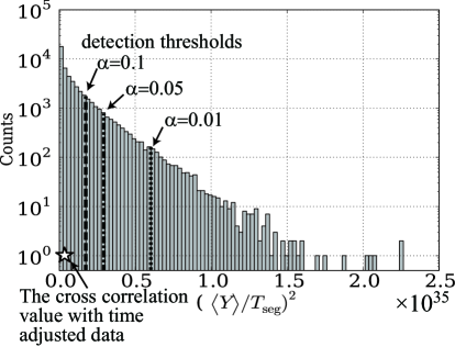
Figure 4: Histogram of $\left(\langle Y\rangle/T_{\rm seg}\right)^{2}$. Dashed and broken lines are detection thresholds with false alarm rates of 10%, 5%, and 1%. The star shows the cross-correlation value with time-adjusted data.

As a result of parameter tuning, data were divided into segments of 200 seconds, and 10% of the segments were removed by the data selection. In total, 206 segments were used to calculate $\langle Y\rangle$. We set the analyzed frequency bandwidth as 0.8 Hz and integrated from 0.035 to 0.830 Hz to calculate $Y$.

Using these parameters, the detection threshold with a false alarm rate of 5% is $|z_{0.05}|=1.7\times 10^{17}$ according to the histogram of $\left(\langle Y\rangle/T_{\rm seg}\right)^{2}$ shown in Fig.4. The cross-correlation value calculated with the time adjusted data is $\langle Y\rangle/T_{\rm seg}=-5.9\times 10^{16}$. Therefore, we concluded that no SGWB signal was detected in our data. As a result of the mock signal injection, our 95 % confidence level upper limit without systematic errors is $\Omega_{\rm gw}h_{0}^{2}<1.7\times 10^{17}$.

The systematic error arises mainly from the overlap reduction function and the calibration. The error in the overlap reduction function occurs because the direction of the test mass is not strictly aligned. We estimate the error in the relative angle of the test masses to be $\pm 5^{\circ}$. Then, the error in the overlap reduction function is 10%. The main reason for the calibration error is the uncertainty of the beam spots on the mirrors. The angular fluctuation of the test mass $\theta$ is derived as $\delta l/L$, where $\delta l$ and $L$ are the change in the beam path length of the interferometer and the distance between the centers of the two mirrors attached at both ends of the test mass. The calibration error appears in $\theta$ because the beam spots are not always on the centers of the two mirrors, which means that $L$ has an error. These errors are estimated to be 10%. Therefore, the total conservative error is $10+10=20$% and our upper limit with 95% confidence level including the error is $\Omega_{\rm gw}h_{0}^{2}\leq 1.9\times 10^{17}$.

Discussion and Future Plans — Considering the integrated upper limits, $\Omega_{\rm gw}h_{0}^{2}$ has already been constrained by the BBN or CMB measurements at 0.035 – 0.830 Hz. However, these upper limits are only on cosmological SGWBs, and not on astronomical SGWBs. Our result is the first to set the upper limit using a direct search constraining both SGWBs in this frequency band.

The result derived from cross-correlation analysis is expected to be better by a factor of $\gamma_{\rm rms}\sqrt{T_{\rm obs}\Delta_{\rm BW}}$ compared to the result derived using a single detector with the same sensitivity, where $\gamma_{\rm rms},T_{\rm obs}$, and $\Delta_{\rm BW}$ are the observation time, the bandwidth of the integration of the cross correlation, and the rms of $\gamma(f)$ over that bandwidth, respectively Abbott et al. (2004). Though $\gamma_{\rm rms}\sqrt{T_{\rm obs}\Delta_{\rm BW}}\sim 1\times 10^{2}$ with our configuration of $\gamma_{\rm rms}\sim 1,\Delta_{\rm BW}=0.8,T_{\rm obs}\sim 2\times 10^{4}{\rm s}$, our result is only about 4 times better than the previous result. This is because we could not achieve the sensitivity obtained in 2009 Ishidoshiro et al. (2011). The poor alignment would induce large coupling noises. Still, we successfully updated the upper limit and extended the explored frequency region due to the uncorrelated noise reduced by the cross-correlation analysis.

For SGWB detection, there is a need to upgrade the setup. Cross correlation analysis using one-year observation data with two TOBAs with a 10 m scaled configuration Ando et al. (2010) should detect a SGWB with $\Omega_{\rm gw}h_{0}^{2}>10^{-8}$. However, it is difficult to achieve such sensitivity at the next upgrade due to several technical problems, such as magnetic coupling noise, seismic coupling noise, thermal noise, and the Newtonian noise. Therefore, we are now constructing a second prototype, Phase-II TOBA. Two orthogonal test masses and an optical bench will be suspended by wires in order to reduce the magnetic coupling noise and common mode noise. In addition to introducing a vibration isolation system, we will monitor the test masses in all the degrees of freedom and diagonalize the signal so that the motion in the pendulum mode will not couple to the signal. The suspension wires will be cooled down for thermal noise reduction. The Newtonian noise Saulson (1984); Hughes and Thorne (1998) would affect the sensitivity of TOBA in the same way as for the interferometric GW detectors and is estimated to be observed below 0.1 Hz with Phase-II TOBA. We will try to test to subtract it using sensor arrays Driggers et al. (2012) because the Newtonian noise cannot be shielded out. Its fundamental sensitivity will be about $h\sim 1\times 10^{-15}/\sqrt{\rm Hz}$ at 1 Hz in strain. Using one-year simultaneous observation data with this sensitivity, the upper limit on a SGWB will be improved to $\Omega_{\rm gw}h_{0}^{2}\leq 1$. Moreover, we will introduce a new method for deriving multiple independent data observed with different directivity. Combining the cross-correlation analysis and this technique, TOBA will have the advantage of mapping a full-sky map of an astronomical SGWB, as well as searching for a cosmological SGWB.

Conclusion — We performed simultaneous 7-hour observations with two prototype TOBAs in Tokyo and Kyoto and searched for a SGWB using cross-correlation analysis. A SGWB signal was not detected and the new 95% confidence upper limit is $\Omega_{\rm gw}h_{0}^{2}\leq 1.9\times 10^{17}$ at 0.035 – 0.830 Hz. This is the first experimental demonstration of a direct SGWB search using cross-correlation analysis with two TOBAs. The results allowed an update of the upper limit and extended exploration of the frequency band.

This work was supported by JSPS KAKENHI Grants No. 24244031, No. 24$\cdot$7531, and No. 25610046.

References

- Buchmüller et al. (2013) W. Buchmüller, V. Domcke, K. Kamada, and K. Schmitz, JCAP 2013, 003 (2013).
- Nakayama et al. (2008) K. Nakayama, S. Saito, Y. Suwa, and J. Yokoyama, JCAP 2008, 020 (2008).
- Abbott et al. (2009) B. Abbott et al., Nature 460, 990 (2009).
- Astone et al. (1999) P. Astone et al., Astron. Astrophys. 351, 811 (1999).
- Akutsu et al. (2008) T. Akutsu et al., Phys. Rev. Lett. 101, 101101 (2008).
- Armstrong et al. (2003) J. W. Armstrong, L. Iess, P. Tortora, and B. Bertotti, The Astrophysical Journal 599, 806 (2003).
- Maggiore (2000) M. Maggiore, Phys. Rep. 331, 283 (2000).
- Allen (1996) B. Allen, Arxiv preprint gr-qc/9604033 (1996).
- Smith et al. (2006) T. L. Smith, E. Pierpaoli, and M. Kamionkowski, Phys. Rev. Lett. 97, 021301 (2006).
- Ando et al. (2010) M. Ando et al., Phys. Rev. Lett. 105, 161101 (2010).
- Ishidoshiro et al. (2011) K. Ishidoshiro et al., Phys. Rev. Lett. 106, 161101 (2011).
- Ishidoshiro et al. (2010) K. Ishidoshiro, M. Ando, A. Takamori, K. Okada, and K. Tsubono, Physica C: Superconductivity 470, 1841 (2010).
- Maggiore (2008) M. Maggiore, Gravitational Waves Volume I Theory and Experiments (Oxford University Press, 2008).
- Helstrom (1968) C. Helstrom, Statistical Theory of Signal Detection: Second Edition, Revised and Enlarged (Pergamon Press, 1968).
- Abbott et al. (2004) B. Abbott et al., Phys. Rev. D 69, 122004 (2004).
- Saulson (1984) P. R. Saulson, Phys. Rev. D 30, 732 (1984).
- Hughes and Thorne (1998) S. A. Hughes and K. S. Thorne, Phys. Rev. D 58, 122002 (1998).
- Driggers et al. (2012) J. C. Driggers, J. Harms, and R. X. Adhikari, Phys. Rev. D 86, 102001 (2012).