A Numerical Study of Methods for Moist Atmospheric Flows: Compressible Equations

Abstract

We investigate two common numerical techniques for integrating reversible moist processes in atmospheric flows in the context of solving the fully compressible Euler equations. The first is a one-step, coupled technique based on using appropriate invariant variables such that terms resulting from phase change are eliminated in the governing equations. In the second approach, which is a two-step scheme, separate transport equations for liquid water and vapor water are used, and no conversion between water vapor and liquid water is allowed in the first step, while in the second step a saturation adjustment procedure is performed that correctly allocates the water into its two phases based on the Clausius-Clapeyron formula. The numerical techniques we describe are first validated by comparing to a well-established benchmark problem. Particular attention is then paid to the effect of changing the time scale at which the moist variables are adjusted to the saturation requirements in two different variations of the two-step scheme. This study is motivated by the fact that when acoustic modes are integrated separately in time (neglecting phase change related phenomena), or when sound-proof equations are integrated, the time scale for imposing saturation adjustment is typically much larger than the numerical one related to the acoustics.

1 Introduction

A key issue in moist atmospheric flow modeling involves the interplay between the dynamics of the flow and the thermodynamics related to reversible and irreversible moist processes. In this paper we focus on reversible processes, i.e. water phase changes, using an exact Clausius-Clapeyron formula for moist thermodynamics, and considering the effects of the specific heats of water and the temperature dependency of the latent heat (as in [18, 16]). Specifically, we want to characterize the impact of modifying the time scale at which the moist thermodynamics is adjusted to the saturation requirements.

Atmospheric flow models are often cast in terms of the potential temperature and Exner function. For moist atmospheres an equivalent potential temperature is typically used as a prognostic variable; see, e.g., [12]. Alternatively, [14], for example, writes the equations of motion in terms of conserved variables, while other thermodynamic variables such as pressure, are recovered diagnostically. This formulation was later extended to include irreversible thermodynamic processes (like precipitation) in [15], and inspired the development of some other conservative schemes considering both primitive variables (e.g., [17, 18, 19]) and a potential temperature-type of formalism (e.g., [11]).

We follow here the approach of [14] in formulating the problem based on the separation of dynamics and thermodynamics. For the dynamics, we explicitly evolve the compressible Euler equations with time steps dictated by the acoustic CFL condition. This allows us to focus on issues of how to couple the moist thermodynamic processes with the dynamics. In particular we can modify the time step associated with the moist thermodynamic adjustments without changing either the formulation of or the numerical solution procedure for the dynamics. In the same spirit, we write the Euler equations in conservation law form (similar to [18]), which eases the inclusion of time-varying thermodynamic parameters for moist air.

Within this formulation, we consider two numerical treatments of moist microphysics (see, e.g., [8]). In the first approach, often referred to as the invariant (conservative) variables approach, the equations of motion are defined using appropriate invariant variables such that terms resulting from phase change are eliminated in the governing equations, while the remaining variables are diagnostically recovered (cf. [9]). (This is the case, for instance, in [14, 15] for total water content and entropy.) In the second approach, which is more common, the equations are again defined using the conservative variable for moist energy, but in this case separate transport equations for liquid water and water vapor are used. The essence of the two-step scheme is that the dynamics are evolved in the first step without allowing any conversion between water vapor and liquid water. In the second step a saturation adjustment procedure is performed that correctly allocates the water into its two phases based on the Clausius-Clapeyron formula (cf. [20]). Similar two-step schemes have been considered, for instance, in [12, 18].

We explore two variants of the two-step scheme. In the first variant, even though liquid water and water vapor are advanced without accounting for phase change, a saturation adjustment procedure is used to diagnose thermodynamic variables such as pressure and the specific heat of moist air that are used to advance the dynamics during the first step. In the second variant, the dynamics is evolved without any adjustment of the water variables or the moist thermodynamics.

Two different questions concerning the time scale for saturation adjustment can be addressed in this way. Using the first variant, we assess the impact of advancing liquid water and water vapor without phase change terms, but with moist dynamics equivalent to that computed with the one-step coupled scheme. Using the second variant, we investigate the impact of completely separating the saturation adjustment from the dynamics.

2 Governing equations

We begin by writing the fully compressible equations of motion expressing conservation of mass, momentum, and energy in a constant gravitational field,

$$\frac{\partial\rho}{\partial t}+\boldsymbol{\nabla}\cdot\left(\rho\boldsymbol{u}\right) = 0,$$ (1)

$$\frac{\partial\left(\rho\boldsymbol{u}\right)}{\partial t}+\boldsymbol{\nabla}\cdot\left(\rho\boldsymbol{u}\boldsymbol{u}\right)+\boldsymbol{\nabla}p = -\rho g\boldsymbol{\hat{e}}_{z},$$ (2)

$$\frac{\partial\left(\rho E\right)}{\partial t}+\boldsymbol{\nabla}\cdot\left(\rho E\boldsymbol{u}+p\boldsymbol{u}\right) = -\rho g\left(\boldsymbol{u}\cdot\boldsymbol{\hat{e}}_{z}\right),$$ (3)

in which we neglect Coriolis forces and viscous terms, as well as the influence of thermal conduction and radiation. Here $\rho$ is the total density and $\boldsymbol{u}$ is the velocity. The energy, $E,$ is defined as the sum of internal plus kinetic energies, and the pressure, $p$, is defined by an equation of state (EOS). We include gravitational acceleration given by $\boldsymbol{g}=-g\boldsymbol{\hat{e}}_{z}$, where $\boldsymbol{\hat{e}}_{z}$ is the unit vector in the vertical direction.

We then follow the formalism as in [16] for moist atmospheres with the additional simplification that at any grid point all phases have the same temperature and velocity. Here we also ignore ice-phase microphysics, precipitation fallout, and subgrid-scale turbulence. We consider an atmosphere with three components, dry air, water vapor, and liquid water, and treat moist air as an ideal mixture with the water phases in thermodynamic equilibrium, so that only reversible processes are taken into account. Denoting by $q_{a}$, $q_{v}$, and $q_{l}$ the mass fraction of dry air, water vapor, and liquid water, respectively, we write

$$\frac{\partial\left(\rho q_{a}\right)}{\partial t}+\boldsymbol{\nabla}\cdot\left(\rho q_{a}\boldsymbol{u}\right) = 0,$$ (4)

$$\frac{\partial\left(\rho q_{v}\right)}{\partial t}+\boldsymbol{\nabla}\cdot\left(\rho q_{v}\boldsymbol{u}\right) = e_{v},$$ (5)

$$\frac{\partial\left(\rho q_{l}\right)}{\partial t}+\boldsymbol{\nabla}\cdot\left(\rho q_{l}\boldsymbol{u}\right) = -e_{v},\enskip.$$ (6)

Since $\rho$ is the total density (i.e. it includes dry air, water vapor and liquid water), we have that $q_{a}+q_{v}+q_{l}=1$. The evaporation rate, $e_{v},$ has dimensions of mass per volume per time; negative values of $e_{v}$ correspond to condensation. Introducing the mass fraction of total water, $q_{w}=q_{v}+q_{l}$, equations (5)–(6) can be also recast as

$$\frac{\partial\left(\rho q_{w}\right)}{\partial t}+\boldsymbol{\nabla}\cdot\left(\rho q_{w}\boldsymbol{u}\right)=0.$$ (7)

The energy $E$ in (3) is defined in this work as

$$E=\widehat{e}+\frac{\boldsymbol{u}\cdot\boldsymbol{u}}{2},$$

where $\widehat{e}$ stands for the specific internal energy of moist air. The constant-volume specific heat of moist air is given by

$$c_{vm}=q_{a}c_{va}+q_{v}c_{vv}+q_{l}c_{vl},$$

with constant specific heats at constant volume: $c_{va}$, $c_{vv}$, and $c_{vl}$, for the three components: air, water vapor, and liquid water, respectively. The internal energy of moist air is thus defined as

$$\widehat{e}=c_{vm}\left(T-T_{\mathrm{trip}}\right)+q_{v}e_{0v},$$ (8)

where $T_{\mathrm{trip}}$ is the triple-point temperature, and $e_{0v}$ is the specific internal energy of water vapor at the triple point. (Following [16], we neglect the contribution of the specific internal energy of dry air at the triple point in the definition of $\widehat{e}$.) [18] considered the same formulation for the internal energy of moist air (8), but included potential energy in the definition of total energy. We note that the definition of $E,$ and in particular of $\widehat{e},$ yields an energy equation (3) with no source terms related to phase changes. In the case of a potential temperature-type of formalism, this can be also achieved by defining a liquid (or ice-liquid) potential temperature as originally introduced by [2, 22], and considered, for instance, in [21, 24, 10, 23].

An equation of state for moist air must be provided to close the system. For the sake of illustration, we consider in this study a standard approach adopted in atmospheric flows in which dry air and water vapor are treated as ideal gases (see, e.g., [14, 18, 11]). The partial pressures of dry air and water vapor are then given by $p_{a}=\rho q_{a}R_{a}T$ and $p_{v}=\rho q_{v}R_{v}T,$ where $R_{a}$ and $R_{v}$ are the specific gas constants for dry air and water vapor, respectively. Denoting by $M_{a}$ and $M_{v}$ the molar masses of dry air and water, respectively, we know that $R_{a}=R/M_{a}$ and $R_{v}=R/M_{v}$, where $R$ is the universal gas constant for ideal gases. If we define the specific gas constant of moist air as

$$R_{m}=q_{a}R_{a}+q_{v}R_{v}=\left(\frac{q_{a}}{M_{a}}+\frac{q_{v}}{M_{v}}\right)R,$$

then the sum of the partial pressures defines the total pressure of a parcel,

$$p=p_{a}+p_{v}=\rho R_{m}T\enskip.$$ (9)

Additionally, the specific heat capacities at constant pressure can be defined as

$$c_{pa}=c_{va}+R_{a},\quad c_{pv}=c_{vv}+R_{v},\quad c_{pm}=c_{vm}+R_{m},$$

for dry air, water vapor, and moist air, respectively. A common approximation in cloud models is to neglect the specific heats of water vapor and liquid water (see, e.g., [3] for a study and discussion on this topic). Here we consider specific heats for all three phases.

Now, the saturation vapor pressure with respect to liquid water, $p_{v}^{*}$, is defined by the following Clausius-Clapeyron relation:

$$p_{v}^{*}(T)=p_{\mathrm{trip}}\left(\frac{T}{T_{\mathrm{trip}}}\right)^{\alpha_{v}}\exp\left[\beta_{v}\left(\frac{1}{T_{\mathrm{trip}}}-\frac{1}{T}\right)\right],$$ (10)

with constants $\alpha_{v}$ and $\beta_{v}$, given, for instance, by

$$\alpha_{v}=\frac{c_{pv}-c_{vl}}{R_{v}},\qquad\beta_{v}=\frac{e_{0v}-(c_{vv}-c_{vl})T_{\mathrm{trip}}}{R_{v}},$$ (11)

as in [16]. The saturated mass fraction of water vapor, $q_{v}^{*}$, can be then computed from the EOS, given in this case by

$$q_{v}^{*}(\rho,T)=\frac{p_{v}^{*}}{\rho R_{v}T}\enskip.$$ (12)

Following [14, 18], we assume that air parcels cannot be supersaturated, and thus water vapor mass fraction, $q_{v}$, cannot exceed its saturated value, $q_{v}^{*}$.

3 Numerical Methodology

In what follows we describe the numerical methodology we use to solve equations (1)–(6) for moist flows. The detailed numerics for dry flow are as described in [1], which describes the CASTRO code, a multicomponent compressible flow solver. Our attention here will be mainly focused on the incorporation of moist reversible processes, and we discuss how the different approaches handle phase transitions within the numerical solution of the overall flow dynamics. We will refer to the first as the one-step coupled scheme, in which the solution variables include energy of moist air and total water, and the effects of phase change are diagnostically evaluated and incorporated when computing the dynamics within each time step. Two variants of the two-step technique will be then studied. In the first one, denoted the two-step semi-split scheme, the density, momentum and energy are evolved exactly as in the one-step fully coupled scheme, but liquid water and water vapor are advected separately and no conversion between them is allowed. In the second one, denoted the two-step fully-split scheme, the dynamics are first evolved neglecting any effects of phase change. In both of the split schemes, the first step is used to advance the solution by one or more time steps before being followed by an adjustment procedure that imposes the saturation requirements using the Clausius-Clapeyron formula, specifically updating $q_{l}$, $q_{v}$, and $T$. Notice that during the first step the water phases may not be in thermodynamic equilibrium anymore; therefore, the saturation adjustment naturally involves an irreversible process. The latter is, however, a result of the numerical approach to approximate moist flows with phase transitions, which are considered as reversible processes in our model. Our formulation and implementation of moist microphysics for the first and second two-step schemes are similar, respectively, to [14] and [18].

In all three cases we define a state vector of conserved variables, ${\bf U},$ and write the time evolution of ${\bf U}$ in the form

$$\frac{\partial{\bf U}}{\partial t}=-\nabla\cdot{\bf F}+{\bf S}_{g},$$

using a finite volume discretization, where ${\bf F}$ is the flux vector and ${\bf S}_{g}$ represents only the gravitational source terms in the equations for momentum and energy. We advance ${\bf U}$ by one time step, $\Delta t,$ using the time discretization,

$${\bf U}^{n+1}={\bf U}^{n}-\Delta t\nabla\cdot{\bf F}^{n+\mathchoice{\kern 0.0pt\raise 1.50694pt\hbox{\sevenrm1}\kern-1.04996pt/\kern-1.04996pt\lower 0.75346pt\hbox{\sevenrm2}}{\kern 0.0pt\raise 1.50694pt\hbox{\sevenrm1}\kern-1.04996pt/\kern-1.04996pt\lower 0.75346pt\hbox{\sevenrm2}}{\kern 0.0pt\raise 1.50694pt\hbox{\fiverm1}\kern-1.39998pt/\kern-1.04996pt\lower 0.75346pt\hbox{\fiverm2}}{1\!/2}}+\Delta t{\bf S}_{g}^{n+\mathchoice{\kern 0.0pt\raise 1.50694pt\hbox{\sevenrm1}\kern-1.04996pt/\kern-1.04996pt\lower 0.75346pt\hbox{\sevenrm2}}{\kern 0.0pt\raise 1.50694pt\hbox{\sevenrm1}\kern-1.04996pt/\kern-1.04996pt\lower 0.75346pt\hbox{\sevenrm2}}{\kern 0.0pt\raise 1.50694pt\hbox{\fiverm1}\kern-1.39998pt/\kern-1.04996pt\lower 0.75346pt\hbox{\fiverm2}}{1\!/2}}.$$ (13)

The total density, $\rho$, as well as $\rho q_{a}$ and $\rho q_{w}$ (or $\rho q_{a},\rho q_{v}$ and $\rho q_{l}$), are included in ${\bf U}$; following the advective update we adjust $q_{a}$ and $q_{w}$ to enforce that $\rho=\rho q_{a}+\rho q_{w}$ (or equivalently $\rho=\rho q_{a}+\rho q_{v}+\rho q_{l}$). The construction of ${\bf F}$ is purely explicit, and based on an unsplit Godunov method with characteristic tracing. The solution, ${\bf U},$ is defined on cell centers; we predict primitive variables, ${\bf Q},$ from cell centers at time $t^{n}$ to edges at time $t^{{n+\mathchoice{\kern 0.0pt\raise 1.50694pt\hbox{\sevenrm1}\kern-1.04996pt/\kern-1.04996pt\lower 0.75346pt\hbox{\sevenrm2}}{\kern 0.0pt\raise 1.50694pt\hbox{\sevenrm1}\kern-1.04996pt/\kern-1.04996pt\lower 0.75346pt\hbox{\sevenrm2}}{\kern 0.0pt\raise 1.50694pt\hbox{\fiverm1}\kern-1.39998pt/\kern-1.04996pt\lower 0.75346pt\hbox{\fiverm2}}{1\!/2}}}$, and use an approximate Riemann solver to construct fluxes ${\bf F}^{n+\mathchoice{\kern 0.0pt\raise 1.50694pt\hbox{\sevenrm1}\kern-1.04996pt/\kern-1.04996pt\lower 0.75346pt\hbox{\sevenrm2}}{\kern 0.0pt\raise 1.50694pt\hbox{\sevenrm1}\kern-1.04996pt/\kern-1.04996pt\lower 0.75346pt\hbox{\sevenrm2}}{\kern 0.0pt\raise 1.50694pt\hbox{\fiverm1}\kern-1.39998pt/\kern-1.04996pt\lower 0.75346pt\hbox{\fiverm2}}{1\!/2}}$ on cell faces. Within the construction of the fluxes, the pressure is diagnostically computed as needed on cell edges using the EOS in (9). As we will see below, the schemes differ in the values of the moist thermodynamic variables that enter this intermediate call to the EOS. This algorithm is formally second-order in both space and time; we refer to [1] for the complete details of this numerical implementation.

The time step in (13) is computed using the standard CFL condition for explicit methods. Following [1], we set a CFL factor $\sigma^{\mathrm{CFL}}$ between 0 and 1, and for a calculation in $n_{\mathrm{dim}}$ dimensions,

$${\Delta t}=\sigma^{\mathrm{CFL}}\min_{i=1\ldots n_{\mathrm{dim}}}\left\{{\Delta t}_{i}\right\},\qquad{\Delta t}_{i}=\frac{\Delta x_{i}}{|{\boldsymbol{u}}_{i}|+c_{m}\;},$$ (14)

with $c_{m}$, the sound speed in moist air, and ${\Delta t}_{i}$ computed as the minimum over all cells. The sound speed is computed using the moist EOS, and is defined in this study as for an ideal gas:

$$c_{m}=\sqrt{\frac{\gamma_{m}p}{\rho}},\qquad\gamma_{m}=\frac{c_{pm}}{c_{vm}},$$

where $\gamma_{m}$ is the isentropic expansion factor of moist air.

In each of the schemes we also need to be able to obtain point-wise values of $(q_{v},q_{l},T)$ given $(\rho,\boldsymbol{u},E,q_{a},q_{w})$, using the Clausius-Clapeyron relation and the saturation requirements. We refer to this as the saturation adjustment procedure, and do so by solving the following nonlinear system of equations [18]:

$$\left.\begin{array}[]{l}\displaystyle\widehat{e}=E-\frac{\boldsymbol{u}\cdot\boldsymbol{u}}{2}=c_{vm}(q_{a},q_{v},q_{l})\left(T-T_{\mathrm{trip}}\right)+q_{v}e_{0v},\\[6.45831pt] q_{v}=\min\left[q_{v}^{*}(\rho,T),q_{w}\right],\\[6.45831pt] q_{l}=q_{w}-q_{v}.\end{array}\right\}$$ (15)

The numerical solution of (15) uses an iterative Newton solver, described in detail here for the sake of completeness:

Step 1:

Initialization. Define the initial guess, $\widetilde{T}=T_{\mathrm{old}}$, where $T_{\mathrm{old}}$ is the last known temperature in the current cell.

Step 2:

Compute mass fractions: $q_{v}$ and $q_{l}$. Following the Clausius-Clapeyron relation (10), compute

$$\widetilde{p_{v}^{*}}\left(\widetilde{T}\right)=p_{\mathrm{trip}}\left(\frac{\widetilde{T}}{T_{\mathrm{trip}}}\right)^{\alpha_{v}}\exp\left[\beta_{v}\left(\frac{1}{T_{\mathrm{trip}}}-\frac{1}{\widetilde{T}}\right)\right],$$

and $\widetilde{q_{v}^{*}}=\widetilde{q_{v}^{*}}(\rho,\widetilde{T})$ from (12), so that

$$\widetilde{q_{v}}=\min\left[\widetilde{q_{v}^{*}},q_{w}\right],\qquad\widetilde{q_{l}}=q_{w}-\widetilde{q_{v}}\enskip.$$

We can then evaluate

$$\widetilde{\widehat{e}}=c_{vm}(q_{a},\widetilde{q_{v}},\widetilde{q_{l}})\left(\widetilde{T}-T_{\mathrm{trip}}\right)+\widetilde{q_{v}}e_{0v}.$$

Step 3:

Update temperature: $T$. Define a local function: $f(\widetilde{T})=\widetilde{\widehat{e}}-\widehat{e}$, and update $\widetilde{T}$ by computing a Newton correction step:

$$\widetilde{T}=\widetilde{T}-\Delta\widetilde{T},\qquad\Delta\widetilde{T}=f(\widetilde{T})/\partial_{\widetilde{T}}f(\widetilde{T}),$$

where

$$\partial_{\widetilde{T}}f=\partial_{\widetilde{T}}q_{v}^{*}(L_{e}(\widetilde{T})-R_{v}\widetilde{T})+c_{vm},\ \partial_{\widetilde{T}}q_{v}^{*}=q_{v}^{*}\left(\frac{\alpha_{v}-1}{\widetilde{T}}+\frac{\beta_{v}}{{\widetilde{T}}^{2}}\right),$$

with the latent heat of vaporization, $L_{e}$, defined as

$$L_{e}(T)=e_{0v}+R_{v}T+(c_{vv}-c_{vl})(T-T_{\mathrm{trip}}).$$ (16)

Step 4:

Stopping criterion. Introducing an accuracy tolerance, $tol$, and denoting $err=|\Delta\widetilde{T}/\widetilde{T}|$, we define the following stopping criterion:

• If $err>tol$: go back to Step 2;

• If $err\leq tol$: stop iterating and set $T=\widetilde{T}$, $q_{v}=\widetilde{q_{v}}$, and $q_{l}=\widetilde{q_{l}}$.

Notice that if $q_{w}<q_{v}^{*}$, all water is in the form of vapor, that is, $q_{v}=q_{w}$ and $q_{l}=0$; the temperature is hence directly computed from (8), or equivalently from Steps 1-4 considering that in this case: $\partial_{\widetilde{T}}f=c_{vm}$. This procedure remains valid for any moist equation of state, as long as a Clausius-Clapeyron relation (10) is available to define the saturation pressure.

We note that for flows in which no phase change occurs, the time evolution of the solution in the one-step and two-step schemes will be identical.

3.1 One-step Coupled Scheme

We consider the following set of evolution equations:

$$\left.\begin{array}[]{rcl}\displaystyle\frac{\partial\rho}{\partial t}+\boldsymbol{\nabla}\cdot\left(\rho\boldsymbol{u}\right)&=&0,\\[6.45831pt] \displaystyle\frac{\partial\left(\rho\boldsymbol{u}\right)}{\partial t}+\boldsymbol{\nabla}\cdot\left(\rho\boldsymbol{u}\boldsymbol{u}\right)+\boldsymbol{\nabla}p&=&-\rho g\boldsymbol{\hat{e}}_{z},\\[6.45831pt] \displaystyle\frac{\partial\left(\rho E\right)}{\partial t}+\boldsymbol{\nabla}\cdot\left(\rho E\boldsymbol{u}+p\boldsymbol{u}\right)&=&-\rho g\left(\boldsymbol{u}\cdot\boldsymbol{\hat{e}}_{z}\right),\\[6.45831pt] \displaystyle\frac{\partial\left(\rho q_{a}\right)}{\partial t}+\boldsymbol{\nabla}\cdot\left(\rho q_{a}\boldsymbol{u}\right)&=&0,\\[6.45831pt] \displaystyle\frac{\partial\left(\rho q_{w}\right)}{\partial t}+\boldsymbol{\nabla}\cdot\left(\rho q_{w}\boldsymbol{u}\right)&=&0,\end{array}\right\}$$ (17)

and close the system with the moist EOS (9). [14] considers the same formulation but the conservation equation for entropy density of moist air is considered instead of $(\rho E)$.

We define the state vector of conserved variables, ${\bf U}=(\rho,\rho\boldsymbol{u},\rho E,\rho q_{a},\rho q_{w});$ the primitive variables in the flux construction are then ${\bf Q}=(\rho,\boldsymbol{u},\rho\widehat{e},q_{a},q_{w}).$ In defining the pressure used to construct the fluxes we solve (15) for $T,$ $q_{v}$, and $q_{l}$, given the values of ${\bf Q}$ before calling the EOS. This approach is coupled in the sense that the moist processes are incorporated as part of the dynamical evolution of the system. Because we evolve $q_{w}$, rather than $q_{v}$ and $q_{l}$ separately, and call the saturation adjustment procedure any time $q_{v}$ and $q_{l}$ are needed, there is never any lagging or neglect of moist effects.

3.2 Two-step Schemes

Here we consider the following set of equations:

$$\left.\begin{array}[]{rcl}\displaystyle\frac{\partial\rho}{\partial t}+\boldsymbol{\nabla}\cdot\left(\rho\boldsymbol{u}\right)&=&0,\\[6.45831pt] \displaystyle\frac{\partial\left(\rho\boldsymbol{u}\right)}{\partial t}+\boldsymbol{\nabla}\cdot\left(\rho\boldsymbol{u}\boldsymbol{u}\right)+\boldsymbol{\nabla}p&=&-\rho g\boldsymbol{\hat{e}}_{z},\\[6.45831pt] \displaystyle\frac{\partial\left(\rho E\right)}{\partial t}+\boldsymbol{\nabla}\cdot\left(\rho E\boldsymbol{u}+p\boldsymbol{u}\right)&=&-\rho g\left(\boldsymbol{u}\cdot\boldsymbol{\hat{e}}_{z}\right),\\[6.45831pt] \displaystyle\frac{\partial\left(\rho q_{a}\right)}{\partial t}+\boldsymbol{\nabla}\cdot\left(\rho q_{a}\boldsymbol{u}\right)&=&0,\\[6.45831pt] \displaystyle\frac{\partial\left(\rho q_{v}\right)}{\partial t}+\boldsymbol{\nabla}\cdot\left(\rho q_{v}\boldsymbol{u}\right)&=&e_{v},\\[6.45831pt] \displaystyle\frac{\partial\left(\rho q_{l}\right)}{\partial t}+\boldsymbol{\nabla}\cdot\left(\rho q_{l}\boldsymbol{u}\right)&=&-e_{v},\end{array}\right\}$$ (18)

where we now define ${\bf U}=(\rho,\rho\boldsymbol{u},\rho E,\rho q_{a},\rho q_{v},\rho q_{l})$ and ${\bf Q}=(\rho,\boldsymbol{u},\rho\widehat{e},q_{a},q_{v},q_{l}).$ We note that, in contrast to the one-step coupled scheme, here we separately advance water vapor and liquid water rather than advancing total water. [18] considers the same setup but an equation for internal energy accounting only for sensible heat is evolved instead of $(\rho E)$; in that formulation a source term corresponding to the latent heat release then appears in the conservation equation for energy. In our case only the equations for $q_{v}$ and $q_{l}$ explicitly contain information about the water phase transitions, which simplifies the comparison of the one- and two-step schemes for the purposes of the present study.

In the first step of both split schemes, $q_{v}$ and $q_{l}$ are advected with $e_{v}=0.$ In the semi-split scheme, the saturation adjustment process is performed before the intermediate pressure is computed from the EOS to define ${\bf F}^{{n+\mathchoice{\kern 0.0pt\raise 1.50694pt\hbox{\sevenrm1}\kern-1.04996pt/\kern-1.04996pt\lower 0.75346pt\hbox{\sevenrm2}}{\kern 0.0pt\raise 1.50694pt\hbox{\sevenrm1}\kern-1.04996pt/\kern-1.04996pt\lower 0.75346pt\hbox{\sevenrm2}}{\kern 0.0pt\raise 1.50694pt\hbox{\fiverm1}\kern-1.39998pt/\kern-1.04996pt\lower 0.75346pt\hbox{\fiverm2}}{1\!/2}}}$, just as in the one-step coupled scheme; the only difference between the procedure here and in the one-step scheme is that we must first define $q_{w}=q_{v}+q_{l}$ before doing the saturation adjustment. In the fully-split scheme, the temperature and pressure are computed for ${\bf F}^{{n+\mathchoice{\kern 0.0pt\raise 1.50694pt\hbox{\sevenrm1}\kern-1.04996pt/\kern-1.04996pt\lower 0.75346pt\hbox{\sevenrm2}}{\kern 0.0pt\raise 1.50694pt\hbox{\sevenrm1}\kern-1.04996pt/\kern-1.04996pt\lower 0.75346pt\hbox{\sevenrm2}}{\kern 0.0pt\raise 1.50694pt\hbox{\fiverm1}\kern-1.39998pt/\kern-1.04996pt\lower 0.75346pt\hbox{\fiverm2}}{1\!/2}}}$ given the existing values of $q_{v}$ and $q_{l}$ on the faces; no saturation adjustment is performed. Given ${\bf F}^{{n+\mathchoice{\kern 0.0pt\raise 1.50694pt\hbox{\sevenrm1}\kern-1.04996pt/\kern-1.04996pt\lower 0.75346pt\hbox{\sevenrm2}}{\kern 0.0pt\raise 1.50694pt\hbox{\sevenrm1}\kern-1.04996pt/\kern-1.04996pt\lower 0.75346pt\hbox{\sevenrm2}}{\kern 0.0pt\raise 1.50694pt\hbox{\fiverm1}\kern-1.39998pt/\kern-1.04996pt\lower 0.75346pt\hbox{\fiverm2}}{1\!/2}}},$ the update in (13) is performed exactly as in the one-step scheme. In the second step of the split schemes we impose the saturation adjustment to correct ${\bf U},$ specifically $q_{v}$ and $q_{l}$, but only if the designated time interval has passed.

In both split schemes, the first step may be performed multiple times before the second step is called. Defining $t_{\mathrm{sat}}$ and $\Delta t_{\mathrm{sat}}$, respectively, as the time at which the saturation adjustment step is performed, and the specified time interval between saturation adjustments, we can describe each of these schemes below.

3.2.1 Two-step Semi-Split Scheme

Step I:

Advance dynamics through ${\Delta t}$. Advance (18) in time from $t^{n}$ to $t^{n+1}=t^{n}+{\Delta t},$ advancing $q_{v}$ and $q_{l}$ with $e_{v}=0,$ but define $q_{w}=q_{v}+q_{l}$ at $t^{n+\mathchoice{\kern 0.0pt\raise 1.50694pt\hbox{\sevenrm1}\kern-1.04996pt/\kern-1.04996pt\lower 0.75346pt\hbox{\sevenrm2}}{\kern 0.0pt\raise 1.50694pt\hbox{\sevenrm1}\kern-1.04996pt/\kern-1.04996pt\lower 0.75346pt\hbox{\sevenrm2}}{\kern 0.0pt\raise 1.50694pt\hbox{\fiverm1}\kern-1.39998pt/\kern-1.04996pt\lower 0.75346pt\hbox{\fiverm2}}{1\!/2}}$ to be used in the saturation adjustment procedure, and compute the intermediate pressure used to construct the fluxes with saturation-adjusted variables.

Step II:

Moist microphysics adjustment. If $t^{n+1}\geq t_{\mathrm{sat}}+\Delta t_{\mathrm{sat}}$, where $t_{\mathrm{sat}}$ records the last time the correction step was computed, solve (15) for $q_{v}$, and $q_{l}$ at $t^{n+1}$ given values of $(\rho,\widehat{e},q_{a},q_{w}=q_{v}+q_{l})$ at $t^{n+1},$ using the iterative procedure described in Steps 1-4. Set $t_{\mathrm{sat}}=t^{n+1}$.

3.2.2 Two-step Fully-Split Scheme

Step I:

Advance dynamics through ${\Delta t}$. Advance (18) in time from $t^{n}$ to $t^{n+1}=t^{n}+{\Delta t}$ with $e_{v}=0.$ In defining the pressure used to construct the fluxes, do not perform the saturation adjustment procedure. Instead, since we explicitly evolve $q_{v}$ and $q_{l}$ separately, compute the temperature, $T,$ directly from (8) (given $E$ and $\boldsymbol{u}$, hence $\widehat{e}$), effectively neglecting any phase change that might occur during the time step. The pressure is then determined from the EOS given these values.

Step II

is exactly as above.

Notice that if $\Delta t_{\mathrm{sat}}\leq{\Delta t}$, the moist and thermodynamic variables are corrected immediately after each update of the dynamics. In the semi-split scheme, the dynamics are evolved with saturation-adjusted variables, but $q_{v}$ and $q_{l}$ themselves drift from their correct values at the end of the time step; the larger $\Delta t_{\mathrm{sat}}$ is, the more they differ from those diagnostically recovered from the one-step solution. In the fully-split scheme, the larger $\Delta t_{\mathrm{sat}}$ is, the more the dynamics evolve neglecting phase changes. Recall that our numerical implementation does not discriminate between fast and slow modes associated with the compressible equations; therefore, whenever $\Delta t_{\mathrm{sat}}>{\Delta t}$, where ${\Delta t}$ is limited by the acoustic CFL condition, several dynamical time steps ${\Delta t}$ are performed before the saturation adjustment.

4 Numerical Simulations

In what follows we first consider the benchmark problem proposed in [3] for moist flows, along with the corresponding configuration for dry air originally presented in [25]. Both cases are presented and results are compared with those obtained in [3] in order to first validate our basic numerical implementation. We then compare the approximations obtained with the different numerical schemes previously described. In particular, we investigate the impact of the time interval of saturation adjustment, $\Delta t_{\mathrm{sat}},$ on the moist flow for the two split schemes. A second configuration based on [7] is also studied for non-isentropic background states and both saturated and only partially saturated media, to further assess the different numerical techniques.

4.1 Numerical Validation

[3] present solutions of a benchmark test case using the fully compressible equations, where the conservation equations for water vapor and liquid water are written in terms of the water vapor and cloud mixing ratios: $r_{v}=q_{v}/q_{a}$ and $r_{c}=q_{l}/q_{a}$, respectively. The conservation equation for energy (3) is replaced by

$$\rho c_{vm}\left(\frac{\partial T}{\partial t}+\boldsymbol{u}\cdot\boldsymbol{\nabla}T\right)=-p\left(\boldsymbol{\nabla}\cdot\boldsymbol{u}\right)-(L_{v}-R_{v}T)e_{v},$$

with the latent heat of vaporization $L_{v}$ defined as

$$L_{v}=L_{v0}-(c_{pl}-c_{pv})(T-T_{0}),$$ (19)

where $L_{v0}$ and $T_{0}$ are constant reference values of $L_{v}$ and $T$, respectively. The nondimensional Exner pressure, $\pi,$ and potential temperature, $\theta,$ are used in [3], defined as

$$\pi=\left(\frac{p}{p_{00}}\right)^{R_{a}/c_{pa}},\qquad\theta=\frac{T}{\pi},$$ (20)

where $p_{00}=1000\,$mb. The numerical scheme thus solves time-dependent equations for $(\boldsymbol{u},\pi,\theta,r_{v},r_{c})$, where the evaporation rate $e_{v}$ appears in the source terms for the equations for $\pi$, $\theta$, $r_{v}$, and $r_{c}$. The technique introduced in [12] is used to integrate the equations in two steps: a dynamical step and the microphysics step. In the dynamical step, $e_{v}$ is neglected and the portions of the governing equations that support acoustic waves are updated with a smaller time step than the other terms. The model is integrated with a third-order Runge-Kutta scheme and fifth-order spatial discretization for the advective terms. Then, a saturation adjustment technique, similar to that proposed by [20], is used in the microphysics step in which only the terms involving phase change are included. Notice that this approach is similar to our fully-split procedure described in § 3.2.2, with the main difference that in our formulation the terms related to phase changes appear only in the equations for $q_{v}$ and $q_{l}$.

The hydrostatic base state pressure can be found through

$$\frac{d\pi_{0}}{dz}=-\frac{g}{c_{pa}\theta_{\rho 0}},$$ (21)

where the subscript “0” stands for hydrostatic base quantities, and the density potential temperature, $\theta_{\rho},$ is defined as

$$\theta_{\rho}=\theta\frac{(1+r_{v}/\epsilon)}{(1+r_{t})},$$ (22)

with the total water mixing ratio, $r_{t}=q_{w}/q_{a}$, and $\epsilon=R_{a}/R_{v}=M_{v}/M_{a}$.

For the next set of computations we consider the following constant parameters, taken from [3]: $R_{a}=287\,$J kg^-1 K^-1, $R_{v}=461\,$J kg^-1 K^-1, $L_{v0}=2.5\times 10^{6}\,$J kg^-1, $c_{va}=717\,$J kg^-1 K^-1, $c_{vv}=1424\,$J kg^-1 K^-1, $c_{pl}=4186\,$J kg^-1 K^-1, $T_{0}=273.15\,$K, and $g=9.81\,$m s^-1. The remaining parameters used in our model are defined such that we have the same definition of the latent heat of vaporization, that is, $L_{v}=L_{e}$ from (19) and (16). Therefore we just need to consider: $T_{\mathrm{trip}}=T_{0}$, $c_{vl}=c_{pl}$, and $e_{0v}=L_{v0}-R_{v}T_{\mathrm{trip}}$. The saturation vapor pressure is computed with the Clausius–Clapeyron equation (10) with constants: $\alpha_{v}=0$ and $\beta_{v}=L_{v0}/R_{v}$, with $p_{\mathrm{trip}}=611\,$Pa, taken from [13] that considers the same benchmark problem.

4.1.1 The Dry Simulation

Following [25] and [3], we consider a two-dimensional computational domain with height $10\,$km and width $20\,$km. The initial atmospheric environment is defined by a constant potential temperature of $\theta_{0}=300\,$K, and the pressure field is obtained by integrating upwards the hydrostatic equation (21). A warm perturbation is introduced in the domain, given by

$$\theta^{\prime}=2\cos^{2}\left(\frac{\pi L}{2}\right),$$ (23)

where

$$L=\min\left\{1,\sqrt{\left(\frac{x-x_{c}}{x_{r}}\right)^{2}+\left(\frac{z-z_{c}}{z_{r}}\right)^{2}}\right\},$$ (24)

with $x_{c}=10\,$km, $z_{c}=2\,$km, and $x_{r}=z_{r}=2\,$km. Notice that our formulation does not use the $\theta-\pi$ formalism; the expressions (20) are used for the conversions, while the initial perturbation (23) is applied at constant pressure $p(z)$. We impose zero normal velocities and homogeneous Neumann boundary conditions for the tangential velocity components on all four boundaries. (Tangential velocity boundary conditions are necessary for the unsplit computation of advective fluxes in this specific numerical solver [1].) For the thermodynamic variables, we impose homogeneous Neumann boundary conditions on the horizontal sides; the background state is reconstructed by extrapolation at vertical boundaries in order to determine the corresponding fluxes.

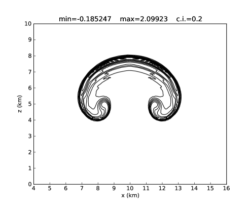
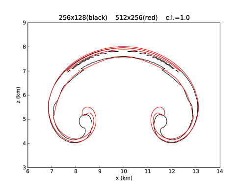
Figure 1: Dry thermal simulation at $1000\,$s. Left: perturbation potential temperature on a $256\times 128$ grid, contoured every $0.2\,$K. Right: comparison of the perturbation potential temperature computed on a $256\times 128$ (black) and $512\times 256$ (red) grids, contours every $1\,$K.

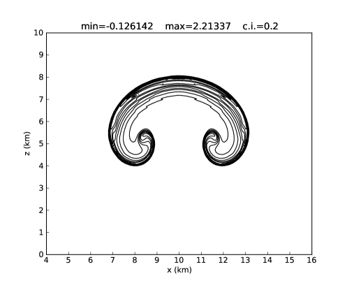
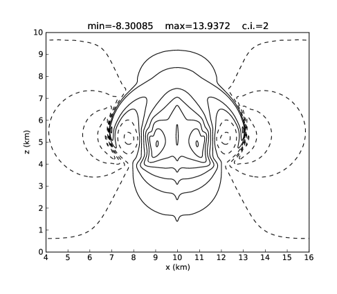
Figure 2: Dry thermal simulation at $1000\,$s on a $512\times 256$ grid. Left: perturbation potential temperature contoured every $0.2\,$K. Right: vertical velocity contoured every $2\,$m s^-1, negative contours are dashed. Contrast to Fig. 1 in [3].

Let us first consider a uniform grid of $256\times 128$ points, slightly finer than the original $100\,$m grid spacing in [3]. For all computations the time step is computed using the CFL factor $\sigma^{\mathrm{CFL}}=0.9$ in (14). This yields roughly constant time steps of about $0.2\,$s in this configuration for the dry thermal computations. Figure 1 (left) illustrates the numerical results for the perturbation potential temperature ($\theta^{\prime}=\theta-\theta_{0}$) after $1000\,$s. The maximum and minimum values for $\theta^{\prime}$ are given by $2.09923\,$K and $-0.18525\,$K, respectively, compared with the original $2.07178\,$K and $-0.144409\,$K in [3]. Good general agreement is also found with respect to the solutions in [3] in terms of the height and width of the rising thermal. However, some differences in the dynamics can be noticed around the two vortices developed on the sides of the thermal. In [3] both tips of the thermal seem to roll up slightly higher around the vortex cores. The maximum and minimum values of vertical velocity are in fact localized in this region, which in our computation are given by $12.4991\,$m s^-1 and $-7.58896\,$m s^-1, respectively, slightly lower than the values of $14.5396\,$m s^-1 and $-8.58069\,$m s^-1 in [3].

Besides the different choice of variables, there are two main differences between our implementation and the one in [3] that may explain the height difference of the thermal tips. The first difference concerns the higher order discretization in both time and space considered in [3]. The second one is given by the numerical decoupling of acoustic waves considered in [3]. Figure 1 (right) shows the same results for $\theta^{\prime}$ and a $256\times 128$ grid, compared with a solution computed using the same numerical scheme this time on a finer grid of $512\times 256$ (consequently, time steps are roughly halved to $0.1\,$s). It can be thus seen that a higher resolution in both time and space compensates for the lower order discretizations and yields better agreement with the solution in [3], as seen in Figure 2. In particular, maximum and minimum values of vertical velocity are this time equal to $13.9372\,$m s^-1 and $-8.30085\,$m s^-1, respectively.

4.1.2 The Moist Simulation

Here we consider the same configuration as above, but now with a moist atmospheric environment. A neutrally stable environment can be obtained by considering the wet equivalent potential temperature $\theta_{e}$, defined for a reversible moist adiabatic atmosphere by

$$\theta_{e}=T\left(\frac{p_{a}}{p_{00}}\right)^{-R_{a}/(c_{pa}+c_{pl}r_{t})}\exp\left[\frac{L_{v}r_{v}}{(c_{pa}+c_{pl}r_{t})T}\right],$$ (25)

taken from [6]. Supposing that the total water mixing ratio is constant at all levels, the vertical profiles of $\pi$, $\theta$, $r_{v}$, and $r_{c}$ can be obtained using (21), (22), and (25), if values for $\theta_{e}$ and $r_{t}$ are provided. We finally compute the hydrostatic base state written in terms of $p$, $T$, $q_{v}$, and $q_{l}$ in our formulation. The value of $r_{t}$ must be greater than $r_{vs}=q_{v}^{*}/q_{a}$, so that the initial environment is saturated, that is, $q_{v}=q_{v}^{*}$ and $q_{l}>0$ everywhere in the domain. The initial perturbation (23) is then introduced in such a way that the buoyancy fields are identical in both the dry and moist simulations, when $\theta_{0}=300\,$K in the dry case [3]. The initial field for $\theta$ is thus given by

$$\theta(p,T)\left(1+\frac{r_{vs}(p,T)}{\epsilon}\right)=\theta_{\rho 0}(1+r_{t})\left(\frac{\theta^{\prime}}{300}+1\right),$$

which is solved pointwise for $T$ throughout the domain at constant pressure $p(z)$.

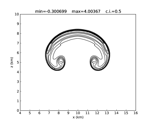
Figure 3: Moist thermal simulation at $1000\,$s. Perturbation potential temperature on a $256\times 128$ grid, contoured every $0.5\,$K.

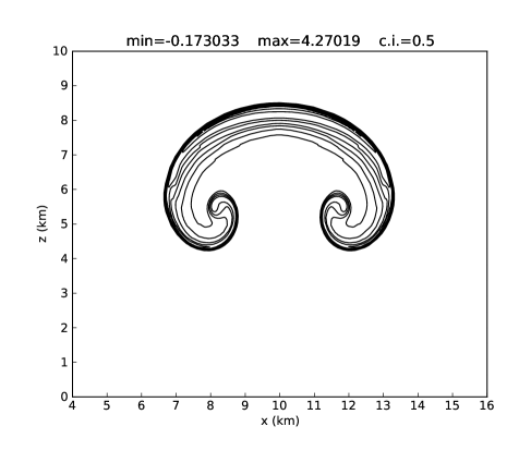
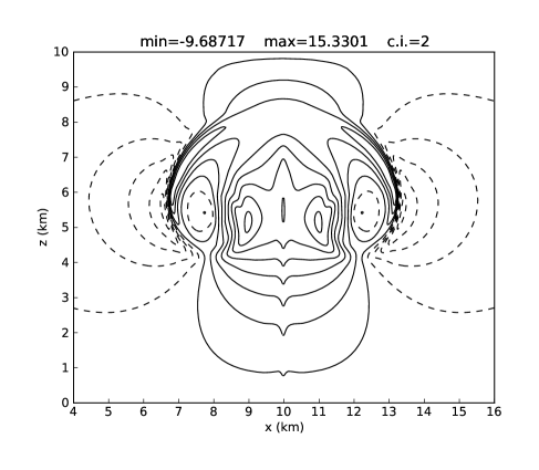
Figure 4: Moist thermal simulation at $1000\,$s on a $512\times 256$ grid. Left: perturbation potential temperature contoured every $0.5\,$K. Right: vertical velocity contoured every $2\,$m s^-1, negative contours are dashed. Contrast to Fig. 3 in [3].

First, we use the one-step coupled scheme described in § 3.1 to compute the moist rising thermal with input parameters: $\theta_{e0}=320\,$K and $r_{t}=0.02$. For a $256\times 128$ grid, time steps are roughly constant of about $0.21\,$s, similar to the dry computation. The introduction of moist microphysics involves an additional cost of approximately $15$ to $20\,$% in CPU time with respect to the dry computation, which roughly corresponds to the computational cost of the Newton iterative procedure, described through Steps 1-4 in Section 3, to solve the nonlinear system (15) throughout the domain. (A fixed tolerance $tol=10^{-10}$ has been used for the Newton solver for all results shown.) The maximum and minimum values for the perturbation wet equivalent potential temperature ($\theta^{\prime}_{e}=\theta_{e}-\theta_{e0}$) are given by $4.00367\,$K and $-0.300699\,$K, respectively, compared with the original $4.09521\,$K and $-0.305695\,$K in [3]. Our computation yields $13.3267\,$m s^-1 and $-8.77365\,$m s^-1, for the maximum and minimum vertical velocities, respectively, which are slightly lower than $15.7130\,$m s^-1 and $-9.92698\,$m s^-1 in [3]. Both solutions look reasonably similar in terms of position, height, and width of the thermal, as seen in Figure 3. Some differences can nevertheless be observed around the vortex cores, as in the previous dry computation. Increasing the spatial and temporal resolution as before yields even better agreement, as seen in Figure 4 for a $512\times 256$ grid. For instance, the maximum and minimum values of vertical velocity are now $15.3301\,$m s^-1 and $-9.68717\,$m s^-1, respectively. These results provide a validation of the numerical implementation of the dynamics solver in conjunction with the moist thermodynamics.

4.2 Comparison of Different Schemes

We now investigate the performance of the two-step schemes detailed in § 3.2 for the moist thermal simulation. In both two-step schemes, the semi-split and the fully-split, the dynamics is advanced allowing no conversion between water vapor and liquid water for a time interval of $\Delta t_{\mathrm{sat}}$ before an adjustment step is performed to account for the saturation requirements. For the purposes of this study, we now consider the reference solution to be that given by the one-step coupled scheme. We focus on evaluating the impact of $\Delta t_{\mathrm{sat}}$ on the results from the split schemes.

4.2.1 Benchmark Problem

We consider again the moist configuration of the benchmark problem in [3]. All simulations were carried out on a uniform grid of $256\times 128$. Recall that the motivation for this study arises from the fact that numerical methods that do not explicitly resolve the acoustic modes typically run with a much larger time step than that required by explicit evolution of the fully compressible equations. Although we continue to resolve the acoustic waves explicitly in this study, we mimic the effect of these larger time steps on the representation of phase changes by increasing $\Delta t_{\mathrm{sat}}.$

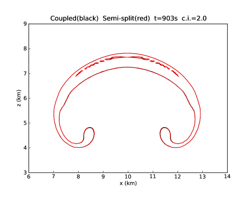
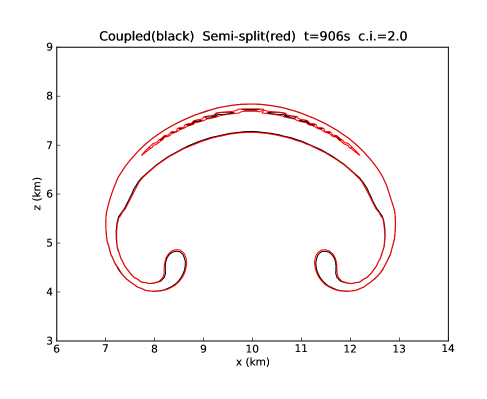
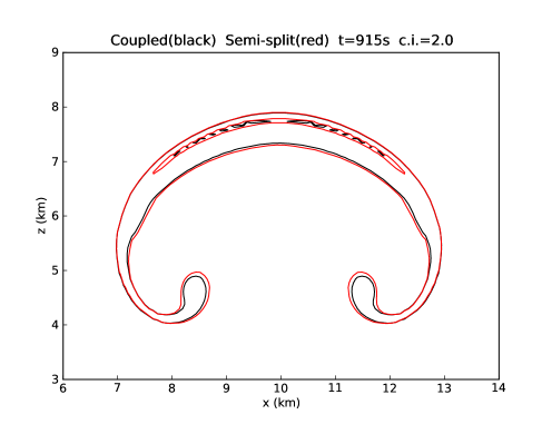
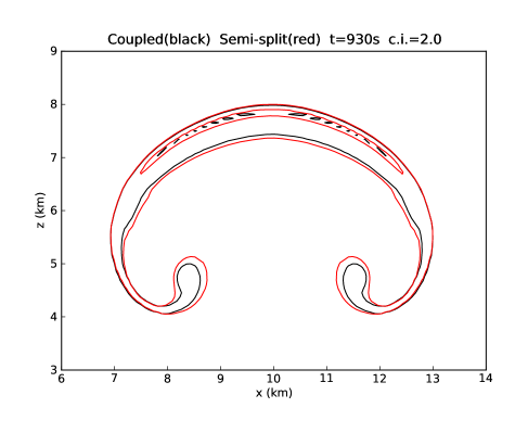
Figure 5: Semi-split solutions for $\theta^{\prime}_{e}$ with $\Delta t_{\mathrm{sat}}=30\,$s and $t_{\mathrm{sat}}=900\,$s each overlaid on the reference solution. Top: $t=903\,$s (left) and $t=906\,$s (right). Bottom: $t=915\,$s (left) and $t=930\,$s (right). Contours every $2\,$K.

Figure 6: Drift of $q_{v}$ computed with the semi-split solver. Time variation of $|\Delta q_{v}/q_{v}^{*}|$ in percentage.

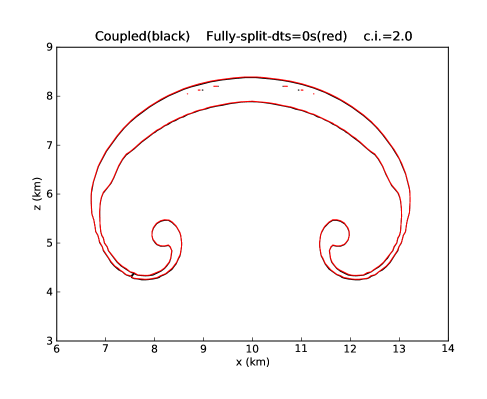
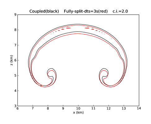
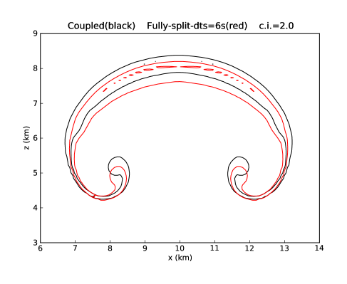
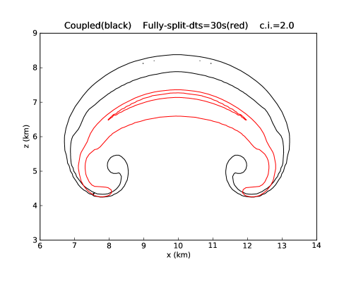
Figure 7: Fully-split solutions for $\theta^{\prime}_{e}$ compared with the coupled ones. Top: $\Delta t_{\mathrm{sat}}=0$ (left) and $\Delta t_{\mathrm{sat}}=3\,$s (right). Bottom: $\Delta t_{\mathrm{sat}}=6\,$s (left) and $\Delta t_{\mathrm{sat}}=30\,$s (right). Contours every $2\,$K.

We first consider the effect of varying $\Delta t_{\mathrm{sat}}$ in the semi-split solver. Regardless of the value of $\Delta t_{\mathrm{sat}},$ the compressible dynamics are still evolved with time steps of about $0.21\,$s. For comparison, we note the time step used by [13] to solve the same problem in a pseudo-incompressible framework was ${\Delta t}=1.66\,$s (corresponding to an advective CFL of $0.5$). As previously noted, the evolution of $\rho$, $\boldsymbol{u}$, and $E$ is identical to that in the one-step coupled scheme. The evolution of liquid water and water vapor neglects phase change, therefore a drift in the values of $q_{v}$ and $q_{l}$ is observed with respect to the reference solution in which the saturation requirements are verified every time step. The semi-split solution drifts from the reference solution, corresponding in this case to the saturated state $q_{v}^{*}$ and $q_{w}-q_{v}^{*}$, only until $t>t_{\mathrm{sat}}+\Delta t_{\mathrm{sat}}$, at which point $q_{v}$ and $q_{l}$ are restored to the same values as in the reference solution, since the dynamics of the semi-split solution are unaffected by the drift. In Figure 5 we present results for $\theta^{\prime}_{e}$ at times $t=903$, $906$, $915$, and $930\,$s, from a simulation with $\Delta t_{\mathrm{sat}}=30\,$s and $t_{\mathrm{sat}}=900\,$s each overlaid on the reference solution. For time $930\,$s, Figure 5 shows the semi-split solution before the saturation adjustment has taken place. Not surprisingly, the larger the time since the last saturation adjustment at $900\,$s, the larger the differences between the semi-split solution and the reference solution. After the adjustment step both solutions are identical. Recall that even though the dynamics and thus the position of the thermals are the same in both cases, $\theta_{e}$ depends on $q_{v}$ and $q_{l}$, via $r_{v}$ and $T$ in (25), which are not the same in both solutions between times $900$ and $930\,$s.

Defining $\Delta q_{v}=q_{v}-q_{v}^{*}$ as the maximum value of the drift over each $\Delta t_{\mathrm{sat}}$ (which occurs when we reach $t^{n+1}\geq t_{\mathrm{sat}}+\Delta t_{\mathrm{sat}}$), we show in Figure 6 the variation of $|\Delta q_{v}/q_{v}^{*}|$ in percentage for simulations with $\Delta t_{\mathrm{sat}}=0$, $3$, $6$, and $30\,$s. Again, not surprisingly, we observe that the maximum drift is roughly proportional to $\Delta t_{\mathrm{sat}}$; when $\Delta t_{\mathrm{sat}}=3\,$s the maximum drift is almost $2\,$%, whereas for $\Delta t_{\mathrm{sat}}=30\,$s the drift reaches almost $20\,$%. For this particular problem, the maximum drifts are due to a local excess of the computed $q_{v}$ with respect to its saturated value. In the simplified set of equations considered here, $q_{v}$ and $q_{l}$ are not used in any other microphysical processes, thus there is no practical impact from the error due to the drift. However, in a more realistic simulation in which the values of $q_{v}$ and $q_{l}$ might enter into other processes, the results here demonstrate that if $\Delta t_{\mathrm{sat}}\gg{\Delta t},$ one must be cautious in the use of $q_{v}$ and $q_{l}$ with lagged saturation adjustment, even if the dynamics is correctly described.

We now consider the effect of $\Delta t_{\mathrm{sat}}\gg{\Delta t}$ on the evolution of the dynamics using the fully-split solver. In Figure 7 we present results from simulations using the fully-split solver and $\Delta t_{\mathrm{sat}}=0$, $3$, $6$, and $30\,$s, again each overlaid on the reference solution. Here we observe that fully neglecting the effect of phase change on the dynamics for long time intervals (relative to the time step numerically defined by the acoustics) allows significant deviations from the reference solution. To quantify this difference, we note that the maximum vertical velocities obtained with the fully-split solver are $13.3267$, $12.9247$, $12.6430$, and $9.40192\,$m s^-1, for $\Delta t_{\mathrm{sat}}=0$, $3$, $6$, and $30\,$s, respectively; whereas the semi-split solver yields $13.3267\,$m s^-1 in all cases, consistent with the coupled reference solution.

4.2.2 Non-isentropic Background State

We consider the hydrostatically balanced profiles in [4] (Eq. 2) for the background state:

$$\left.\begin{array}[]{l}\theta_{0}(z)=\theta_{00}\exp(Sz),\\[6.45831pt] \displaystyle p_{0}(z)=p_{00}\left[1-\frac{g}{c_{pa}\theta_{00}S}\left(1-\exp(-Sz)\right)\right]^{c_{pa}/R_{a}},\end{array}\right\}$$ (26)

where $\theta_{00}$ and $p_{00}$ stand for the environmental potential temperature and pressure at the surface ($z=0$), with the static stability $S$ defined as $S=N^{2}/g=d\ln\theta_{0}/dz$ ($N$ is the Brunt-Väisälä frequency). The potential temperature is given by (20). For the following computations we define a computational domain $4\,$km high and wide, with periodic horizontal boundary conditions and the same vertical boundary conditions implemented for the previous benchmark problem. The same thermodynamic parameters from [3] are considered, whereas constants (11) coming from [16] are considered in the Clausius–Clapeyron equation (10) with $p_{\mathrm{trip}}=611\,$Pa. From [7], we take $S=1.3\times 10^{-5}\,$m^-1, $\theta_{00}=283\,$K, and $p_{00}=850\,$hPa. All simulations were performed on a uniform grid of $256\times 256$.

For our formulation we also need to compute the hydrostatic base density $\rho_{0}$ based on the background temperature and pressure (26), and the distribution of air, water vapor, and liquid water in the atmosphere. The latter quantities are set by the relative humidity in the atmosphere RH measured in percentage and defined as RH$~{}=(p_{v}/p_{v}^{*})\times 100$. In particular if RH${}_{0}<100\,$%, then no liquid water should be present in the atmosphere in order to guarantee the thermodynamic equilibrium of the initial state, that is, $q_{l0}(z)=0$. We consider in this study two cases: first, a saturated medium, that is RH${}_{0}=100\,$% and $r_{t}=0.02$, just like in the moist benchmark problem; and a second configuration with RH${}_{0}=20\,$%, and hence, no liquid water in the initial background state. Contrary to the benchmark configuration in [3], we now have in either case a non-isentropic background state, where the following definitions of specific entropy have been adopted [16]:

$$s_{a} = c_{pa}\log\left(\frac{T}{T_{\mathrm{trip}}}\right)-R_{a}\log\left(\frac{p}{p_{\mathrm{trip}}}\right),$$

$$s_{v} = c_{pv}\log\left(\frac{T}{T_{\mathrm{trip}}}\right)-R_{v}\log\left(\frac{p}{p_{\mathrm{trip}}}\right)+S_{0v},$$

$$s_{l} = c_{vl}\log\left(\frac{T}{T_{\mathrm{trip}}}\right),$$

$$s_{m} = q_{a}s_{a}+q_{v}s_{v}+q_{l}s_{l},$$ (27)

for dry air, water vapor, liquid water, and moist air, with $S_{0v}=e_{0v}/T_{\mathrm{trip}}+R_{v}$. (Notice that the specific entropy of dry air at the triple point is neglected in this definition.)

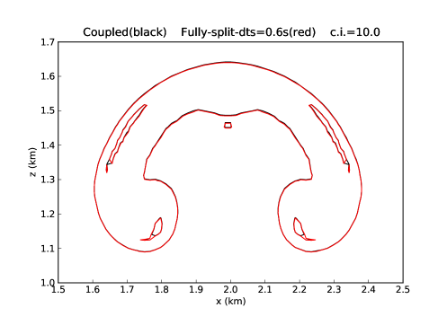
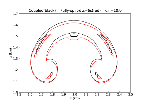
Figure 8: Initially saturated, non-isentropic background state. Fully-split solutions for $s_{m}$ after $300\,$s with $\Delta t_{\mathrm{sat}}=0.6\,$s (left) and $\Delta t_{\mathrm{sat}}=6\,$s (right), compared with the coupled ones. Contours every $10\,$J kg^-1 K^-1.

Let us consider the first configuration with an initially saturated environment. In this case the moist squared Brunt-Väisälä frequency $N_{m}^{2}$ can be computed according to [5] (eqs. 36–37), which yields $N_{m}^{2}$ monotonically varying from $3.5\times 10^{-6}\,$s^-2 at the surface up to $1.3\times 10^{-5}\,$s^-2 at the top of the computational domain. Positive values of $N_{m}^{2}$ imply static moist stability. Similar to (23), we introduce a warm perturbation on temperature:

$$T^{\prime}=2\cos^{2}\left(\frac{\pi L}{2}\right),$$ (28)

where $L$ is defined by (24), with $x_{c}=2\,$km, $z_{c}=0.8\,$km, and $x_{r}=z_{r}=300\,$m. The water distributions, as well as the density, are thus adjusted to the perturbed temperature with the original pressure field. As for the previous problem both the coupled and the split schemes with $\Delta t_{\mathrm{sat}}=0$, yield the same solutions, with $\sigma^{\mathrm{CFL}}=0.9$ and roughly constant time steps of about $0.04\,$s. Increasing $\Delta t_{\mathrm{sat}}$ in the fully-split scheme has a comparable effect to that seen in the benchmark problem with an isentropic base state. Figure 8 illustrates the latter behavior in terms of the specific entropy of moist air (eq. (27)) for $\Delta t_{\mathrm{sat}}=0.6$ and $6\,$s, after $300\,$s of integration. Simulations were stopped before the nonlinearities become more apparent and sub-grid turbulence starts playing a more important role in the dynamics, as analyzed in [7]. We recall that for the sake of simplicity sub-grid turbulence is not considered in the present study. We note that the choice of $\Delta t_{\mathrm{sat}}=0.6\,$s is based on the approximate size of the time step that would be used if computed from the advective rather than acoustic CFL condition, i.e. if the time step were based on the fluid velocity rather than the sound speed.

For the second configuration with RH${}_{0}=20\,$%, we consider the same temperature perturbation (28) and an additional circular perturbation on the relative humidity, which is set to $100\,$% for a radius $r<200\,$m, as considered in [7]. A transition layer is assumed such that

$${\rm RH}={\rm RH}_{0}+(100-{\rm RH}_{0})\cos^{2}\left(\frac{\pi}{2}\frac{r-200}{100}\right),\ 200\leq r\leq 300,$$ (29)

taken also from [7]. Initially there is no liquid water in the domain, not even in the saturated region, whereas the perturbed water vapor is recomputed based on (28) and (29) with the original static pressure. After performing the same tests with the different numerical techniques, the same observations can be made in terms of moist saturation adjustments. For instance, Figure 9 shows results obtained with the fully-split scheme with an adjustment interval of $\Delta t_{\mathrm{sat}}=6\,$s; once again $\sigma^{\mathrm{CFL}}=0.9$, which yields roughly constant time steps of about $0.04\,$s. Notice that in this case, differences between the fully-split and coupled approximations are smaller with respect to the previous configurations for saturated and both isentropic and non-isentropic environments. This is due to the fact that all the liquid water is mainly contained in the perturbed area and hence only this region is subjected to phase changes and active moist microphysics.

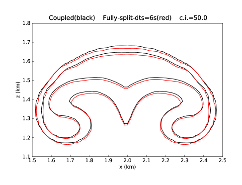
Figure 9: Non-isentropic background state with a partially saturated perturbation. Fully-split solution for $s_{m}$ after $300\,$s with $\Delta t_{\mathrm{sat}}=6\,$s compared with the coupled one. Contours every $50\,$J kg^-1 K^-1.

5 Summary

In this paper we have studied the incorporation of reversible moist processes related to phase change phenomena into numerical simulations of atmospheric flows. Specifically, we have tried to characterize the impact of modifying the time scale at which the moist thermodynamics is adjusted to the saturation requirements. For the purpose of this study, the compressible Euler equations were written in a form including conservation equations for total density, momentum, and energy of moist air, and were explicitly evolved with time steps dictated by the acoustic CFL condition.

Two different approaches were considered to evolve the system. In the first approach, a one-step coupled procedure solves the equations of motion together with a conservation equation for total water content. Because of the choice of variables, in particular because the energy of moist air includes the contribution of both sensible and latent heats, this formulation does not include source terms related to phase change in either the energy or the total water equation. Therefore, the system of equations can be solved without needing to estimate or neglect source terms related to phase change. The pressure used to update the momentum and energy in the evolution equations is computed from the equation of state following a saturation adjustment procedure.

In the second approach, the evolution equation for total water is replaced by separate evolution equations for liquid water and water vapor, where source terms related to phase change now appear. A two-step technique is implemented in which the system of equations is first evolved with these source terms set to zero. In a second step, a saturation adjustment procedure is performed after a time interval $\Delta t_{\mathrm{sat}}$, updating the values of liquid water and water vapor. We consider two variants of the two-step scheme. In the first, a semi-split strategy in which the dynamics of the moist flow are correctly computed, a drift is expected and observed in the values of water vapor and liquid water during the time interval in which the saturation adjustment is not imposed. In the second, fully-split scheme, the saturation adjustment is not performed during the evolution of the dynamics, and the dynamics themselves are seem to drift from those of the fully coupled solution.

In summary, numerical tests of the semi-split scheme showed that non-trivial deviations of the water vapor and liquid water from their correct values may occur even when the dynamics is correctly described. Tests of the fully-split scheme demonstrated that imposing the saturation adjustment too infrequently relative to the time step at which the dynamics evolve may lead to inaccuracies in the dynamical evolution. Further testing with both isentropic and non-isentropic background states, as well as saturated and non-saturated initial configurations, confirmed the initial findings. It is hoped that the insight gained here as to how closely the saturation adjustment should be numerically coupled to the dynamics will carry over to methods in which the dynamics themselves are evolved with larger time steps. This will be further investigated and discussed in future work.

References

- [1] A. S. Almgren, V. E. Beckner, J. B. Bell, M. S. Day, L. H. Howell, C. C. Joggerst, M. J. Lijewski, A. Nonaka, M. Singer, and M. Zingale. CASTRO: A new compressible astrophysical solver. I. Hydrodynamics and self-gravity. ApJ, 715:1221–1238, 2010.
- [2] A. K. Betts. Non‐precipitating cumulus convection and its parameterization. Quart. J. Roy. Meteor. Soc., 99(419):178–196, 1973.
- [3] G. H. Bryan and J. M. Fritsch. A benchmark simulation for moist nonhydrostatic numerical models. Mon. Wea. Rev., 130:2917–2928, 2002.
- [4] T. L. Clark and R. D. Farley. Severe downslope windstorm calculations in two and three spatial dimensions using anelastic interactive grid nesting: A possible mechanism for gustiness. J. Atmos. Sci., 41:329–350, 1984.
- [5] D. R. Durran and J. B. Klemp. On the effects of moisture on the Brunt-Väisälä frequency. J. Atmos. Sci, 39:2152–2158, 1982.
- [6] K. A. Emanuel. Atmospheric Convection. Oxford University Press, 1994.
- [7] W. W. Grabowski and T. L. Clark. Cloud-environment interface instability: Rising thermal calculations in two spatial dimensions. J. Atmos. Sci., 48:527–546, 1991.
- [8] W. W. Grabowski and P. K. Smolarkiewicz. Monotone finite-difference approximations to the advection-condensation problem. Mon. Weather Rev., 118:2082–2097, 1990.
- [9] T. Hauf and H. Höller. Entropy and potential temperature. J. Atmos. Sci., 44:2887–2901, 1989.
- [10] H. Jiang and W. R. Cotton. Large eddy simulation of shallow cumulus convection during BOMEX: Sensitivity to microphysics and radiation. J. Atmos. Sci., 57:582–594, 2000.
- [11] J. B. Klemp, W. C. Skamarock, and J. Dudhia. Conservative split-explicit time integration methods for the compressible nonhydrostatic equations. Mon. Wea. Rev., 135:2897–2913, 2007.
- [12] J. B. Klemp and R. B. Wilhelmson. The simulation of three-dimensional convective storm dynamics. J. Atmos. Sci., 35:1070–1096, 1978.
- [13] W. P. O’Neill and R. Klein. A moist pseudo-incompressible model. Atmos. Res., 142:133–141, 2014.
- [14] K. V. Ooyama. A thermodynamic foundation for modeling the moist atmosphere. J. Atmos. Sci., 47:2580–2593, 1990.
- [15] K. V. Ooyama. A dynamic and thermodynamic foundation for modeling the moist atmosphere with parameterized microphysics. J. Atmos. Sci., 58:2073–2102, 2001.
- [16] D. M. Romps. The dry-entropy budget of a moist atmosphere. J. Atmos. Sci., 65:3779–3799, 2008.
- [17] M. Satoh. Conservative scheme for the compressible nonhydrostatic models with the horizontally explicit and vertically implicit time integration scheme. Mon. Wea. Rev., 130:1227–1245, 2002.
- [18] M. Satoh. Conservative scheme for a compressible nonhydrostatic model with moist processes. Mon. Wea. Rev., 131:1033–1050, 2003.
- [19] M. Satoh, T. Matsuno, H. Tomita, H. Miura, T. Nasuno, and S. Iga. Nonhydrostatic icosahedral atmospheric model (NICAM) for global cloud resolving simulations. J. Comput. Phys., 227:3486–3514, 2008.
- [20] S.-T. Soong and Y. Ogura. A comparison between axisymmetric and slab-symmetric cumulus cloud models. J. Atmos. Sci., 30:879–893, 1973.
- [21] G. J. Tripoli. A nonhydrostatic mesoscale model designed to simulate scale interaction. Mon. Wea. Rev., 120:1342–1359, 1992.
- [22] G. J. Tripoli and W. R. Cotton. The use of lce-liquid water potential temperature as a thermodynamic variable in deep atmospheric models. Mon. Wea. Rev., 109:1094–1102, 1981.
- [23] R. L. Walko and R. Avissar. The Ocean-Land-Atmosphere Model (OLAM). Part II: Formulation and tests of the nonhydrostatic dynamic core. Mon. Wea. Rev., 136:4045–4062, 2008.
- [24] R. L. Walko, W. R. Cotton, G. Feingold, and B. Stevens. Efficient computation of vapor and heat diffusion between hydrometeors in a numerical model. Atmos. Res., 53(1–3):171–183, 2000.
- [25] L. J. Wicker and W. C. Skamarock. A time-splitting scheme for the elastic equations incorporating second-order Runge–Kutta time differencing. Mon. Wea. Rev., 126:1992–1999, 1998.