Multiscale Stochastic Volatility Model for Derivatives on Futures

Abstract

In this paper we present a new method to compute the first-order approximation of the price of derivatives on futures in the context of multiscale stochastic volatility of Fouque et al. (2011, CUP). It provides an alternate method to the singular perturbation technique presented in Hikspoors and Jaimungal (2008). The main features of our method are twofold: firstly, it does not rely on any additional hypothesis on the regularity of the payoff function, and secondly, it allows an effective and straightforward calibration procedure of the model to implied volatilities. These features were not achieved in previous works. Moreover, the central argument of our method could be applied to interest rate derivatives and compound derivatives. The only pre-requisite of our approach is the first-order approximation of the underlying derivative. Furthermore, the model proposed here is well-suited for commodities since it incorporates mean reversion of the spot price and multiscale stochastic volatility. Indeed, the model was validated by calibrating it to options on crude-oil futures, and it displays a very good fit of the implied volatility.

1 Introduction

In many financial applications the underlying asset of the derivative contract under consideration is a derivative itself. A very important example of this complex and widely traded class of products consists of derivatives on future contracts. We shall study such financial instruments in the context of multiscale stochastic volatility as presented in Fouque et al. (2011).

It is well-known that under the No-Arbitrage Hypothesis, one can find a risk-neutral probability measure such that all tradable assets in this market, when properly discounted, are martingales under this measure (see Delbaen and Schachermayer (2008) for an extensive exposition on this subject). Here, we assume constant interest rate throughout this paper.

The future contract on the asset $V$ with maturity $T$ is a standardized contract traded at a futures exchange for which both parties consent to trade the asset $V$ at time $T$ for a price agreed upon the day the contract was written. This previously arranged price is called strike. The future price at time $t$ with maturity $T\geq t$ of the asset $V$, which will be denoted by $F_{t,T}$, is defined as the strike of the future contract on $V$ with maturity $T$ such that no premium is paid at time $t$. In symbols,

(1.1) $$F_{t,T}=\mathbb{E}_{\mathbb{Q}}[V_{T}\ |\ \mathcal{F}_{t}],$$

where $\mathbb{Q}$ is a risk-neutral probability. If the asset $V$ is tradable, then we simply have $F_{t,T}=e^{r(T-t)}V_{t}$, where $r$ is the constant interest rate, and then derivatives on futures can be treated in the exact same way one handles derivatives on the asset itself.

When interest rate is constant, future prices are non-trivial when the asset is not tradable and therefore the discounted asset price is not a martingale, see for example (Musiela and Rutkowski, 2008, Chapter 3). This will be our main assumption: the asset $V$ is not tradable. More precisely, we assume the asset price presents mean reversion. Some examples of such assets are: commodities, currency exchange rates, volatility indices, and interest rates.

Empirical evidence of the presence of stochastic factors in the volatility of financial assets is greatly documented in the literature, see for example Gatheral (2006) and references therein. The presence of a fast time-scale in the volatility in the S&P 500 was reported in Fouque et al. (2003b). We refer the reader to Fouque et al. (2011) for comprehensive exposition on this subject. Multiscale stochastic volatility models lead to a first-order approximation of derivatives prices. This approximation is composed by the leading-order term given by the Black-Scholes price with the averaged effective volatility and the first-order correction only involves Greeks of this leading-term. In terms of implied volatility, this perturbation analysis translates into an affine approximation in the log-moneyness to maturity ratio (LMMR). Subsequently, this leads to a simple calibration procedure of the group market parameters, that are also used to compute the first-order approximation of the price of exotic derivatives.

Because of the nature of our problem, the future price, which is the underlying asset of the derivative in consideration, has its dynamics explicitly depending on the time-scales of the volatility. This creates an important difference from the usual perturbation theory to the derivative pricing problem.

The method presented in this paper can be described as follows:

• Write the stochastic differential equation (SDE) for the future $F_{t,T}$ with all coefficients depending only on $F_{t,T}$. This means we will need to invert the future prices of $V$ in order to write $V_{t}$ as a function of $F_{t,T}$.

• Consider the pricing partial differential equation (PDE) for a European derivative on $F_{t,T}$. The coefficients of this PDE will depend on the time-scales of the stochastic volatility of the asset in a complicated way. At this point, we use perturbation analysis to treat such PDE by expanding the coefficients.

• Determine the first-order approximation of derivatives on $F_{t,T}$ as it is done in Fouque et al. (2011).

Indeed, this method is not the only way to tackle this problem. Instead, we could have considered this compound derivative as a more elaborate derivative in the asset and then find the first-order approximation proposed in Hikspoors and Jaimungal (2008). This, in turn, follows the idea designed in Cotton et al. (2004) and is based on the Taylor expansion of the payoff under consideration around the zero-order term of the approximation of the future price $F_{t,T}$. Therefore, some smoothness of the payoff function must be assumed. Since the method considered here does not rely on such Taylor expansion, no restriction other than the ones intrinsic to the perturbation method is required. Furthermore, we shall show that although the method presented here is more involved, it allows a cleaner calibration. This is due to the fact we are considering the derivative as a function of the future price, which is a tradable asset and hence a martingale under the pricing risk-neutral measure. We refer to Section 5 for a more thoroughly comparison between our method introduced here and the method presented in Hikspoors and Jaimungal (2008).

Another important set of examples that can be handled using the method proposed in this paper consists of interest rate derivatives (see Cotton et al. (2004)). Moreover, in the equity case, the method could be use to tackle the general problem of pricing compound derivatives, as it is done in Fouque and Han (2005) by Taylor expansion of the payoff function.

The main contribution of our work is a general method to compute the first-order approximation of the price of general compound derivatives such that no additional hypothesis on the regularity of the payoff function must be assumed. The only pre-requisite is the first-order approximation of the underlying derivative. In other words, the method proposed here allows us to derive the first-order approximation of compound derivatives keeping the hypotheses of the original approximation given in Fouque et al. (2011). Furthermore, this method maintains another desirable feature of the perturbation method: the direct calibration of the market group parameters.

This paper is organized as follows: Section 2 describes the dynamics of the underlying asset and then, in Section 3 we follow the method previously outlined to find the first-order approximation of derivatives on future contracts of $V$. Section 4 characterizes the calibration procedure to call options and we analyze an example of calibration to options on crude-oil futures. Finally, we conclude the paper in Sections 5 and 6 with a comparison of our work with a previous method and some suggestions for further research.

2 The Model

Firstly, we fix a filtered risk-neutral probability space $(\Omega,\mathcal{F},(\mathcal{F}_{t})_{t\geq 0},\mathbb{Q})$. The risk-neutral measure is chosen so that the relation (1.1) holds. In this probability space, we assume that the asset value $V_{t}$ is described by an exponential Ornstein-Uhlenbeck (exp-OU) stochastic process with a multiscale stochastic volatility. Namely,

(2.8) $$\left\{\begin{array}[]{l}V_{t}=e^{s(t)+U_{t}},\\ \\ dU_{t}=\kappa(m-U_{t})dt+\eta(Y^{\varepsilon}_{t},Z^{\delta}_{t})dW_{t}^{(0)},\\ \\ \displaystyle dY^{\varepsilon}_{t}=\frac{1}{\varepsilon}\alpha(Y_{t}^{\varepsilon})dt+\frac{1}{\sqrt{\varepsilon}}\beta(Y_{t}^{\varepsilon})dW_{t}^{(1)},\\ \\ dZ^{\delta}_{t}=\delta c(Z^{\delta}_{t})dt+\sqrt{\delta}g(Z^{\delta}_{t})dW_{t}^{(2)},\\ \end{array}\right.$$

where $(W_{t}^{(0)},W_{t}^{(1)},W_{t}^{(2)})$ is a correlated $\mathbb{Q}$-Brownian motion with

$$dW_{t}^{(0)}dW_{t}^{(i)}=\raisebox{1.5pt}{$\rho$}_{i}dt,\ i=1,2,\ dW_{t}^{(1)}dW_{t}^{(2)}=\raisebox{1.5pt}{$\rho$}_{12}dt.$$

We shall denote by $Y^{1}$ the process given by the second of the stochastic differential equations in (2.8) when $\varepsilon=1$.

The main assumptions of this model are:

1. There exists a unique solution of the SDE (2.8) for any fixed $(\varepsilon,\delta)$.

2. The risk-neutral probability $\mathbb{Q}$ is chosen in order to match the future prices of $V$ observed in the market to the prices produced by the model (2.8) and the martingale relation (1.1).

3. $|\raisebox{1.5pt}{$\rho$}_{1}|<1$, $|\raisebox{1.5pt}{$\rho$}_{2}|<1$, $|\raisebox{1.5pt}{$\rho$}_{12}|<1$ and $1+2\raisebox{1.5pt}{$\rho$}_{1}\raisebox{1.5pt}{$\rho$}_{2}\raisebox{1.5pt}{$\rho$}_{12}-\raisebox{1.5pt}{$\rho$}_{1}^{2}-\raisebox{1.5pt}{$\rho$}_{2}^{2}-\raisebox{1.5pt}{$\rho$}_{12}^{2}>0$. These conditions ensure the positive definiteness of the covariance matrix of $(W_{t}^{(0)},W_{t}^{(1)},W_{t}^{(2)})$.

4. The interest rate is constant and equals $r$.

5. $\alpha$ and $\beta$ are such that the process $Y^{1}$ has a unique invariant distribution and is mean-reverting as in (Fouque et al., 2011, Section 3.2).

6. $\eta(y,z)$ is a positive function, smooth in $z$ and such that $\eta^{2}(\cdot,z)$ is integrable with respect to the invariant distribution of $Y^{1}$.

7. $s(t)$ is a deterministic seasonality factor.

It is important to notice that we could have explicitly considered the market prices of volatility risk as it is done in Fouque et al. (2011) and in doing so we would have a term of order $\varepsilon^{-1/2}$ and a term of order $\delta^{1/2}$ in the drifts of $Y^{\varepsilon}$ and $Z^{\delta}$ respectively, both depending on $Y^{\varepsilon}$ and $Z^{\delta}$, and they could have been handled in the way it is done in the aforesaid reference. For simplicity of notation, we do not consider these market prices of volatility risk here.

A simple generalization of this model is the addition of a deterministic time-varying long run mean $m(t)$ in the drift of $U$, which can be easily handled. A more subtle extension would be to the Schwartz two-factor model, see Schwartz (1997).

We now restate the definition of the future prices of $V$

(2.9) $$F_{t,T}=\mathbb{E}_{\mathbb{Q}}[V_{T}\ |\ \mathcal{F}_{t}],\ 0\leq t\leq T,$$

and then in next the section we will develop the first-order approximation of derivatives on $F_{t,T}$.

Remark 2.1.

More precisely, we say that a function $g^{\varepsilon,\delta}$ is a first-order approximation to the function $f^{\varepsilon,\delta}$ if

$$|g^{\varepsilon,\delta}-f^{\varepsilon,\delta}|\leq C(\varepsilon+\delta),$$

pointwise for some constant $C>0$ and for sufficiently small $\varepsilon,\delta>0$. We use the notation

(2.10) $$g^{\varepsilon,\delta}-f^{\varepsilon,\delta}=O(\varepsilon+\delta).$$

3 Derivatives on Future Contracts

3.1 First-Order Approximation for Future Prices

Here, we present the first-order approximation of future prices on mean-reverting assets. For a fixed maturity $T>0$, we define

$$h^{\varepsilon,\delta}(t,u,y,z,T)=\mathbb{E}_{\mathbb{Q}}[V_{T}\ |\ U_{t}=u,Y^{\varepsilon}_{t}=y,Z^{\delta}_{t}=z],$$

and note that $F_{t,T}=h^{\varepsilon,\delta}(t,U_{t},Y_{t}^{\varepsilon},Z_{t}^{\delta},T)$. We consider the formal expansion in powers of $\sqrt{\varepsilon}$ and $\sqrt{\delta}$ of $h^{\varepsilon,\delta}$:

$$h^{\varepsilon,\delta}(t,u,y,z,T)=\sum_{i,j\geq 0}(\sqrt{\varepsilon})^{i}(\sqrt{\delta})^{j}h_{i,j}(t,x,y,z,T).$$

We are interested in the first-order approximation of derivatives on mean-reverting assets, which is presented in Hikspoors and Jaimungal (2008) and Chiu et al. (2011). Remember $Y^{1}$ denotes the process $Y^{\varepsilon}$ with $\varepsilon=1$.

Applying the first-order approximation of future prices described in the aforesaid references, we choose the first terms of the above formal series to be

(3.1) $$h_{0}(t,u,z,T)=\exp\left\{s(T)+m+(u-m)e^{-\kappa(T-t)}+\frac{\bar{\eta}^{2}(z)}{4\kappa}\left(1-e^{-2\kappa(T-t)}\right)\right\},$$

(3.2) $$h_{1,0}(t,u,z,T)=g(t,T)V_{3}(z)\frac{\partial^{3}h_{0}}{\partial u^{3}}(t,u,z,T),$$

(3.3) $$h_{0,1}(t,u,z,T)=f(t,T)V_{1}(z)\frac{\partial^{3}h_{0}}{\partial u^{3}}(t,u,z,T),$$

where, denoting the averaging with respect to the invariant distribution of $Y^{1}$ by $\langle\cdot\rangle$, we have

(3.4) $$\bar{\eta}^{2}(z) =\langle\eta^{2}(\cdot,z)\rangle,$$

(3.5) $$V_{3}(z) =-\frac{\raisebox{1.5pt}{$\rho$}_{1}}{2}\left\langle\eta(\cdot,z)\beta(\cdot)\frac{\partial\phi}{\partial y}(\cdot,z)\right\rangle,$$

(3.6) $$V_{1}(z) =\raisebox{1.5pt}{$\rho$}_{2}g(z)\langle\eta(\cdot,z)\rangle\bar{\eta}(z)\bar{\eta}^{\prime}(z),$$

(3.7) $$f(t,T) =\frac{e^{3\kappa(T-t)}-e^{2\kappa(T-t)}}{2\kappa^{2}}-\frac{e^{3\kappa(T-t)}-1}{6\kappa^{2}},$$

(3.8) $$g(t,T) =\frac{e^{-3\kappa(T-t)}-1}{3\kappa},$$

and $\phi(y,z)$ is the solution of the Poisson equation

(3.9) $$\mathcal{L}_{0}\phi(y,z)=\eta^{2}(y,z)-\bar{\eta}^{2}(z),$$

with $\mathcal{L}_{0}$ being the infinitesimal generator of $Y^{1}$. Moreover, we may assume $h_{1,1}$ does not depend on $y$ and choose

(3.10) $$h_{2,0}(t,u,y,z,T)=-\frac{1}{2}\phi(y,z)\frac{\partial^{2}h_{0}}{\partial u^{2}}(t,u,z,T)+c(t,u,z,T),$$

for some function $c$ that does not depend on $y$. Under all these choices and some regularity conditions similar to the ones presented in Theorem 3.2 at the end of this section, as it was shown in Chiu et al. (2011) and Hikspoors and Jaimungal (2008), we have

$$h^{\varepsilon,\delta}(t,u,y,z)= \,\,h_{0}(t,u,z,T)+\sqrt{\varepsilon}h_{1,0}(t,u,z,T)+\sqrt{\delta}h_{0,1}(t,u,z,T)+O(\varepsilon+\delta).$$

Furthermore, the following simplifications hold:

$$h_{1,0}(t,u,z,T)=g(t,T)V_{3}(z)e^{-3\kappa(T-t)}h_{0}(t,u,z,T),$$

and

$$h_{0,1}(t,u,z,T)=f(t,T)V_{1}(z)e^{-3\kappa(T-t)}h_{0}(t,u,z,T).$$

3.2 The Dynamics of the Future Prices

In this section, we will derive the SDE describing the dynamics of $F_{t,T}$ and write its coefficients as functions of $F_{t,T}$. Since $F_{t,T}$ is a martingale under $\mathbb{Q}$, its dynamics has no drift and hence, applying Itô’s Formula to $F_{t,T}=h^{\varepsilon,\delta}(t,U_{t},Y^{\varepsilon}_{t},Z^{\delta}_{t},T)$, we get

$$dF_{t,T} =\frac{\partial h^{\varepsilon,\delta}}{\partial u}(t,U_{t},Y_{t}^{\varepsilon},Z_{t}^{\delta},T)\eta(Y^{\varepsilon}_{t},Z^{\delta}_{t})dW_{t}^{(0)}$$

$$+\frac{1}{\sqrt{\varepsilon}}\frac{\partial h^{\varepsilon,\delta}}{\partial y}(t,U_{t},Y_{t}^{\varepsilon},Z_{t}^{\delta},T)\beta(Y_{t}^{\varepsilon})dW_{t}^{(1)}$$

$$+\sqrt{\delta}\frac{\partial h^{\varepsilon,\delta}}{\partial z}(t,U_{t},Y_{t}^{\varepsilon},Z_{t}^{\delta},T)g(Z^{\delta}_{t})dW_{t}^{(2)}.$$

We are interested in derivatives contracts on $F_{t,T}$ and in applying the perturbation method to approximate their prices. Thus, we will rewrite the SDE above with all coefficients depending on $F_{t,T}$ instead of $U_{t}$. In order to proceed, we assume we can invert $h^{\varepsilon,\delta}$ with respect to $u$ for fixed $\varepsilon,\delta,y,z$ and $T$, i.e. there exists a function $H^{\varepsilon,\delta}(t,x,y,z,T)$ such that

$$H^{\varepsilon,\delta}(t,\cdot,y,z,T)=(h^{\varepsilon,\delta}(t,\cdot,y,z,T))^{-1}\mbox{ .}$$

Since $h_{0}(t,u,z)$ given by (3.1) is invertible in $u$, at least for small $\varepsilon$ and $\delta$, this inversion is not a strong assumption on our model. The asymptotic analysis of $H^{\varepsilon,\delta}$ is given in the following lemma.

Lemma 3.1.

If we choose $H_{0}$, $H_{1,0}$, $H_{0,1}$ to be

• $H_{0}(t,\cdot,z,T)=(h_{0}(t,\cdot,z,T))^{-1},$
  

• $\displaystyle H_{1,0}(t,x,z,T)=-\frac{h_{1,0}(t,H_{0}(t,x,z,T),z,T)}{\displaystyle\frac{\partial h_{0}}{\partial u}(t,H_{0}(t,x,z,T),z,T)},$
  

• $\displaystyle H_{0,1}(t,x,z,T)=-\frac{h_{0,1}(t,H_{0}(t,x,z,T),z,T)}{\displaystyle\frac{\partial h_{0}}{\partial u}(t,H_{0}(t,x,z,T),z,T)},$

where $h_{1,0}$ and $h_{0,1}$ are given by (3.2) and (3.3) respectively, then, we have

$$H^{\varepsilon,\delta}(t,x,y,z,T) =H_{0}(t,x,z,T)+\sqrt{\varepsilon}H_{1,0}(t,x,z,T)+\sqrt{\delta}H_{0,1}(t,x,z,T)+O(\varepsilon+\delta).$$

Proof.

The derivation is straightforward. ∎

Notice that $H^{\varepsilon,\delta}(t,F_{t,T},y,z,T)=U_{t}$ and if we define

(3.11) $$\psi^{\varepsilon,\delta}_{1}(t,x,y,z,T) =\frac{\partial h^{\varepsilon,\delta}}{\partial u}(t,H^{\varepsilon,\delta}(t,x,y,z,T),y,z,T),$$

(3.12) $$\psi^{\varepsilon,\delta}_{2}(t,x,y,z,T) =\frac{\partial h^{\varepsilon,\delta}}{\partial y}(t,H^{\varepsilon,\delta}(t,x,y,z,T),y,z,T),$$

(3.13) $$\psi^{\varepsilon,\delta}_{3}(t,x,y,z,T) =\frac{\partial h^{\varepsilon,\delta}}{\partial z}(t,H^{\varepsilon,\delta}(t,x,y,z,T),y,z,T),$$

we obtain the desired SDE for $F_{t,T}$

(3.14) $$dF_{t,T} =\psi^{\varepsilon,\delta}_{1}(t,F_{t,T},Y_{t}^{\varepsilon},Z_{t}^{\delta},T)\eta(Y^{\varepsilon}_{t},Z^{\delta}_{t})dW_{t}^{(0)}$$

$$+\frac{1}{\sqrt{\varepsilon}}\psi^{\varepsilon,\delta}_{2}(t,F_{t,T},Y_{t}^{\varepsilon},Z_{t}^{\delta},T)\beta(Y_{t}^{\varepsilon})dW_{t}^{(1)}$$

$$+\sqrt{\delta}\psi^{\varepsilon,\delta}_{3}(t,F_{t,T},Y_{t}^{\varepsilon},Z_{t}^{\delta},T)g(Z^{\delta}_{t})dW_{t}^{(2)}.$$

3.3 A Pricing PDE for Derivatives on Future Contracts

We now fix a future contract on $V$ with maturity $T$ and consider a European derivative with maturity $T_{0}<T$ and whose payoff $\varphi$ depends only on the terminal value $F_{T_{0},T}$. A no-arbitrage price for this derivative on $F_{t,T}$ is given by

$$P^{\varepsilon,\delta}(t,x,y,z,T)=\mathbb{E}_{\mathbb{Q}}[e^{-r(T_{0}-t)}\varphi(F_{T_{0},T})\ |\ F_{t,T}=x,Y^{\varepsilon}_{t}=y,Z^{\delta}_{t}=z],$$

where $\mathbb{Q}$ is the risk-neutral probability discussed in Section 2 and we are using the fact that $(F_{t,T},Y^{\varepsilon}_{t},Z^{\delta}_{t})$ is a Markov process. In this section we derive a PDE for $P^{\varepsilon,\delta}$. Recall that $F_{t,T}$ follows Equation (3.14), where $Y_{t}^{\varepsilon}$ and $Z_{t}^{\delta}$ are given in (2.8). Then, we write the infinitesimal generator $\mathcal{L}^{\varepsilon,\delta}$ of $(F_{t,T},Y^{\varepsilon}_{t},Z^{\delta}_{t})$, where, for simplicity of notation, we will drop the variables $(t,x,y,z,T)$ of $\psi_{i}^{\varepsilon,\delta}$, $i=1,2,3$,

(3.15) $$\hskip 14.22636pt\mathcal{L}^{\varepsilon,\delta} =\frac{1}{\varepsilon}\left(\mathcal{L}_{0}+\frac{1}{2}(\psi^{\varepsilon,\delta}_{2})^{2}\beta^{2}(y)\frac{\partial^{2}}{\partial x^{2}}+\psi^{\varepsilon,\delta}_{2}\beta^{2}(y)\frac{\partial^{2}}{\partial x\partial y}\right)$$

$$+\frac{1}{\sqrt{\varepsilon}}\left(\raisebox{1.5pt}{$\rho$}_{1}\psi^{\varepsilon,\delta}_{1}\psi^{\varepsilon,\delta}_{2}\eta(y,z)\beta(y)\frac{\partial^{2}}{\partial x^{2}}+\raisebox{1.5pt}{$\rho$}_{1}\psi^{\varepsilon,\delta}_{1}\eta(y,z)\beta(y)\frac{\partial^{2}}{\partial x\partial y}\right)$$

$$+\frac{\partial}{\partial t}+\frac{1}{2}(\psi^{\varepsilon,\delta}_{1})^{2}\eta^{2}(y,z)\frac{\partial^{2}}{\partial x^{2}}-r\cdot$$

$$+\sqrt{\delta}\left(\raisebox{1.5pt}{$\rho$}_{2}\psi^{\varepsilon,\delta}_{1}\psi^{\varepsilon,\delta}_{3}\eta(y,z)g(z)\frac{\partial^{2}}{\partial x^{2}}+\raisebox{1.5pt}{$\rho$}_{2}\psi^{\varepsilon,\delta}_{1}\eta(y,z)g(z)\frac{\partial^{2}}{\partial x\partial z}\right)$$

$$+\delta\left(\mathcal{M}_{2}+\frac{1}{2}(\psi^{\varepsilon,\delta}_{3})^{2}g^{2}(z)\frac{\partial^{2}}{\partial x^{2}}+\psi^{\varepsilon,\delta}_{3}g^{2}(z)\frac{\partial^{2}}{\partial x\partial z}\right)$$

$$+\sqrt{\frac{\delta}{\varepsilon}}\left(\raisebox{1.5pt}{$\rho$}_{12}\psi^{\varepsilon,\delta}_{2}\psi^{\varepsilon,\delta}_{3}\beta(y)g(z)\frac{\partial^{2}}{\partial x^{2}}+\raisebox{1.5pt}{$\rho$}_{12}\psi^{\varepsilon,\delta}_{3}\beta(y)g(z)\frac{\partial^{2}}{\partial x\partial y}\right.$$

$$\hskip 34.14322pt\left.+\raisebox{1.5pt}{$\rho$}_{12}\psi^{\varepsilon,\delta}_{2}\beta(y)g(z)\frac{\partial^{2}}{\partial x\partial z}+\raisebox{1.5pt}{$\rho$}_{12}\beta(y)g(z)\frac{\partial^{2}}{\partial y\partial z}\right),$$

where

(3.16) $$\mathcal{L}_{0}=\frac{1}{2}\beta^{2}(y)\frac{\partial^{2}}{\partial y^{2}}+\alpha(y)\frac{\partial}{\partial y},$$

(3.17) $$\mathcal{M}_{2}=\frac{1}{2}g^{2}(z)\frac{\partial^{2}}{\partial z^{2}}+c(z)\frac{\partial}{\partial z}.$$

It is well-known that under some mild conditions, by Feynman-Kac’s Formula, $P^{\varepsilon,\delta}$ satisfies the pricing PDE

(3.21) $$\left\{\begin{array}[]{l}\mathcal{L}^{\varepsilon,\delta}P^{\varepsilon,\delta}(t,x,y,z,T)=0,\\ \\ P^{\varepsilon,\delta}(T_{0},x,y,z,T)=\varphi(x).\end{array}\right.$$

3.4 Perturbation Framework

We will now develop the formal singular and regular perturbation analysis for European derivatives on $F_{t,T}$ following the method outlined in Fouque et al. (2011). However, in our case we have a fundamental difference: the coefficients of the differential operator $\mathcal{L}^{\varepsilon,\delta}$, given by Equation (3.15), depend on $\varepsilon$ and $\delta$ in an intricate way. In particular, the term corresponding to the factor $\varepsilon^{-1}$ is not simply of order $\varepsilon^{-1}$. To circumvent this problem, we will expand the coefficients in powers of $\varepsilon$ and $\delta$ and then collect the correct terms for each order. Therefore, it will be necessary to compute some terms of the expansion of $\psi_{i}^{\varepsilon,\delta}$. All the details for this expansion are given in the Appendix A and the final result is:

$$\mathcal{L}^{\varepsilon,\delta}=\frac{1}{\varepsilon}\mathcal{L}_{0}+\frac{1}{\sqrt{\varepsilon}}\mathcal{L}_{1}+\mathcal{L}_{2}+\sqrt{\varepsilon}\mathcal{L}_{3}+\sqrt{\delta}\mathcal{M}_{1}+\sqrt{\frac{\delta}{\varepsilon}}\mathcal{M}_{3}+\cdots,$$

where $\mathcal{L}_{0}$ is given by (3.16) and

(3.22) $$\hskip 28.45274pt\mathcal{L}_{1} =\raisebox{1.5pt}{$\rho$}_{1}e^{-\kappa(T-t)}\eta(y,z)\beta(y)x\frac{\partial^{2}}{\partial x\partial y},$$

(3.23) $$\hskip 28.45274pt\mathcal{L}_{2} =\frac{\partial}{\partial t}+\frac{1}{2}e^{-2\kappa(T-t)}\eta^{2}(y,z)x^{2}\frac{\partial^{2}}{\partial x^{2}}-r\cdot$$

$$-\frac{1}{2}e^{-2\kappa(T-t)}\frac{\partial\phi}{\partial y}(y,z)\beta^{2}(y)x\frac{\partial^{2}}{\partial x\partial y},$$

(3.24) $$\hskip 28.45274pt\mathcal{M}_{3} =\raisebox{1.5pt}{$\rho$}_{12}\frac{(1-e^{-2\kappa(T-t)})}{2\kappa}\beta(y)g(z)\bar{\eta}(z)\bar{\eta}^{\prime}(z)x\frac{\partial^{2}}{\partial x\partial y}$$

$$+\raisebox{1.5pt}{$\rho$}_{12}\beta(y)g(z)\frac{\partial^{2}}{\partial y\partial z},$$

(3.25) $$\hskip 28.45274pt\mathcal{L}_{3} =(\psi_{2,3,0}(t,x,y,z,T)\beta^{2}(y)$$

$$+\raisebox{1.5pt}{$\rho$}_{1}\psi_{1,2,0}(t,x,y,z,T)\eta(y,z)\beta(y))\frac{\partial^{2}}{\partial x\partial y}$$

$$-\raisebox{1.5pt}{$\rho$}_{1}\frac{1}{2}e^{-3\kappa(T-t)}\frac{\partial\phi}{\partial y}(y,z)\eta(y,z)\beta(y)x^{2}\frac{\partial^{2}}{\partial x^{2}},$$

(3.26) $$\hskip 28.45274pt\mathcal{M}_{1} =\raisebox{1.5pt}{$\rho$}_{2}e^{-\kappa(T-t)}\frac{(1-e^{-2\kappa(T-t)})}{2\kappa}\eta(y,z)g(z)\bar{\eta}(z)\bar{\eta}^{\prime}(z)x^{2}\frac{\partial^{2}}{\partial x^{2}}$$

$$+\raisebox{1.5pt}{$\rho$}_{2}e^{-\kappa(T-t)}\eta(y,z)g(z)x\frac{\partial^{2}}{\partial x\partial z}+(\psi_{2,2,1}(t,x,y,z,T)\beta^{2}(y)$$

$$+\raisebox{1.5pt}{$\rho$}_{2}\psi_{1,1,1}(t,x,T)\eta(y,z)\beta(y))\frac{\partial^{2}}{\partial x\partial y}.$$

The fundamental difference with the situation described in Fouque et al. (2011) then materializes in one term: the differential operator $\mathcal{L}_{3}$ which contributes to the order $\sqrt{\varepsilon}$ in the expansion of $\mathcal{L}^{\varepsilon,\delta}$. Also, observe that the coefficients of these operators are time dependent which complicates the asymptotic analysis. This difficulty has also been dealt with in Fouque et al. (2004).

3.5 Formal Derivation of the First-Order Approximation

Let us formally write $P^{\varepsilon,\delta}$ in powers of $\sqrt{\delta}$ and $\sqrt{\varepsilon}$,

$$P^{\varepsilon,\delta}=\sum_{m,k\geq 0}(\sqrt{\varepsilon})^{k}(\sqrt{\delta})^{m}P_{k,m},$$

and denote $P_{0,0}$ simply by $P_{0}$ where we assume that, at maturity $T_{0}$, $P_{0}(T_{0},x,y,z,T)=\varphi(x)$. We are interested in determining $P_{0}$, $P_{1,0}$ and $P_{0,1}$. We follow the method presented in Fouque et al. (2011) with some minor modifications in order to take into account the new term $\mathcal{L}_{3}$.

In order to compute the leading term $P_{0}$ and $P_{1,0}$, we set to be zero the following terms of the expansion of $\mathcal{L}^{\varepsilon,\delta}P^{\varepsilon,\delta}$:

(3.27) $$(-1,0): \ \mathcal{L}_{0}P_{0}=0,$$

(3.28) $$(-1/2,0): \ \mathcal{L}_{0}P_{1,0}+\mathcal{L}_{1}P_{0}=0,$$

(3.29) $$(0,0): \ \mathcal{L}_{0}P_{2,0}+\mathcal{L}_{1}P_{1,0}+\mathcal{L}_{2}P_{0}=0,$$

(3.30) $$(1/2,0): \ \mathcal{L}_{0}P_{3,0}+\mathcal{L}_{1}P_{2,0}+\mathcal{L}_{2}P_{1,0}+\mathcal{L}_{3}P_{0}=0,$$

where we are using the notation $(i,j)$ to denote the term of $i$th order in $\varepsilon$ and $j$th in $\delta$.

3.5.1 Computing $P_{0}$

We seek a function $P_{0}=P_{0}(t,x,z,T)$, independent of $y$, so that the Equation (3.27) is satisfied. Since $\mathcal{L}_{1}$ takes derivative with respect to $y$, $\mathcal{L}_{1}P_{0}=0$. Thus the second (3.28) becomes $\mathcal{L}_{0}P_{1,0}=0$ and for the same reason as before, we seek a function $P_{1,0}=P_{1,0}(t,x,z,T)$ independent of $y$. The $(0,0)$-order equation (3.29) becomes

$$\mathcal{L}_{0}P_{2,0}+\cancelto{\scriptstyle 0}{\mathcal{L}_{1}P_{1,0}}+\mathcal{L}_{2}P_{0}=0,$$

which is a Poisson equation for $P_{2,0}$ with solvability condition

$$\langle\mathcal{L}_{2}P_{0}\rangle=0,$$

where $\langle\cdot\rangle$ is the average under the invariant measure of $\mathcal{L}_{0}$. For more details on Poisson equations, see (Fouque et al., 2011, Section 3.2). Define now

(3.31) $$\mathcal{L}_{B}(\sigma)=\frac{\partial}{\partial t}+\frac{1}{2}\sigma^{2}x^{2}\frac{\partial^{2}}{\partial x^{2}}-r\cdot$$

and

(3.32) $$\sigma(t,y,z,T)=e^{-\kappa(T-t)}\eta(y,z),$$

where we are using the notation $\mathcal{L}_{B}(\sigma)$ for the Black differential operator with volatility $\sigma$. Since $P_{0}$ does not depend on $y$ and by the form of $\mathcal{L}_{2}$ given in (3.23), the solvability condition becomes

$$\langle\mathcal{L}_{2}P_{0}\rangle=\langle\mathcal{L}_{B}(\sigma(t,y,z,T))\rangle P_{0}=0.$$

Note that

$$\langle\mathcal{L}_{B}(\sigma(t,y,z,T))\rangle=\frac{\partial}{\partial t}+\frac{1}{2}x^{2}\left\langle\sigma^{2}(t,\cdot,z,T)\right\rangle\frac{\partial^{2}}{\partial x^{2}}-r\cdot=\mathcal{L}_{B}(\bar{\sigma}(t,z,T)),$$

where

(3.33) $$\bar{\sigma}^{2}(t,z,T)=\left\langle\sigma^{2}(t,\cdot,z,T)\right\rangle=e^{-2\kappa(T-t)}\bar{\eta}^{2}(z),$$

with $\bar{\eta}(z)$ defined in (3.4). Therefore, we choose $P_{0}$ to satisfy the PDE

(3.37) $$\left\{\begin{array}[]{l}\mathcal{L}_{B}(\bar{\sigma}(t,z,T))P_{0}(t,x,z,T)=0,\\ \\ P_{0}(T_{0},x,z,T)=\varphi(x).\end{array}\right.$$

Note also that $\mathcal{L}_{B}(\bar{\sigma}(t,z,T))$ is the Black differential operator with time-varying volatility $\bar{\sigma}(t,z,T)$ and hence, if we define the time-averaged volatility, $\bar{\sigma}_{t,T_{0}}(z,T)$, by the formula

(3.38) $$\bar{\sigma}^{2}_{t,T_{0}}(z,T) =\frac{1}{T_{0}-t}\int_{t}^{T_{0}}\bar{\sigma}^{2}(u,z,T)du$$

$$=\bar{\eta}^{2}(z)\left(\frac{e^{-2\kappa(T-T_{0})}-e^{-2\kappa(T-t)}}{2\kappa(T_{0}-t)}\right),$$

we can write

$$P_{0}(t,x,z,T)=P_{B}(t,x,\bar{\sigma}_{t,T_{0}}(z,T)),$$

where $P_{B}(t,x,\sigma)$ is the price at $(t,x)$ of the European derivative with maturity $T_{0}$ and payoff function $\varphi$ in the Black model with constant volatility $\sigma$.

In order to simplify notation here and in what follows, we define

(3.39) $$\lambda(t,T_{0},T,\kappa) =\frac{e^{-\kappa(T-T_{0})}-e^{-\kappa(T-t)}}{\kappa(T_{0}-t)}.$$

Therefore,

(3.40) $$\bar{\sigma}^{2}_{t,T_{0}}(z,T)=\bar{\eta}^{2}(z)\lambda_{\sigma}^{2}(t,T_{0},T,\kappa),$$

where

(3.41) $$\lambda_{\sigma}(t,T_{0},T,\kappa) =\sqrt{\lambda(t,T_{0},T,2\kappa)}.$$

3.5.2 Computing $P^{\varepsilon}_{1,0}$

By the $(0,0)$-order equation (3.29), we get the formula

(3.42) $$P_{2,0}=-\mathcal{L}_{0}^{-1}(\mathcal{L}_{B}(\sigma)-\mathcal{L}_{B}(\bar{\sigma}))P_{0}+c(t,x,z,T),$$

for some function $c$ which does not depend on $y$. Denote by $\phi(y,z)$ a solution of the Poisson equation

$$\mathcal{L}_{0}\phi(y,z)=\eta^{2}(y,z)-\bar{\eta}^{2}(z).$$

Hence,

$$\mathcal{L}_{0}^{-1}(\mathcal{L}_{B}(\sigma)-\mathcal{L}_{B}(\bar{\sigma})) =\mathcal{L}_{0}^{-1}\left(\frac{1}{2}(\sigma^{2}(t,y,z,T)-\bar{\sigma}^{2}(t,z,T))x^{2}\frac{\partial^{2}}{\partial x^{2}}\right)$$

$$=\frac{1}{2}e^{-2\kappa(T-t)}\mathcal{L}_{0}^{-1}(\eta^{2}(y,z)-\bar{\eta}^{2}(z))x^{2}\frac{\partial^{2}}{\partial x^{2}}$$

$$=\frac{1}{2}e^{-2\kappa(T-t)}\phi(y,z)D_{2},$$

where we use the notation

(3.43) $$D_{k}=x^{k}\frac{\partial^{k}}{\partial x^{k}}.$$

From the $(1/2,0)$-order equation (3.30), which is a Poisson equation for $P_{3,0}$, we get the solvability condition

(3.44) $$\langle\mathcal{L}_{1}P_{2,0}+\mathcal{L}_{2}P_{1,0}+\mathcal{L}_{3}P_{0}\rangle=0.$$

Using formula (3.42) for $P_{2,0}$ and formula (3.22) for $\mathcal{L}_{1}$, we get

$$\mathcal{L}_{1}P_{2,0} =-\mathcal{L}_{1}\mathcal{L}_{0}^{-1}(\mathcal{L}_{B}(\sigma)-\mathcal{L}_{B}(\bar{\sigma}))P_{0}$$

$$=-\raisebox{1.5pt}{$\rho$}_{1}e^{-\kappa(T-t)}\eta(y,z)\beta(y)x\frac{\partial^{2}}{\partial x\partial y}\left(\frac{1}{2}e^{-2\kappa(T-t)}\phi(y,z)D_{2}P_{0}\right)$$

$$=-\raisebox{1.5pt}{$\rho$}_{1}e^{-\kappa(T-t)}x\eta(y,z)\beta(y)\frac{\partial}{\partial x}\frac{\partial}{\partial y}\left(\frac{1}{2}e^{-2\kappa(T-t)}\phi(y,z)D_{2}P_{0}\right)$$

$$=-\frac{1}{2}\raisebox{1.5pt}{$\rho$}_{1}e^{-3\kappa(T-t)}\eta(y,z)\beta(y)\frac{\partial\phi}{\partial y}(y,z)D_{1}D_{2}P_{0}.$$

We also have by equation (3.23)

$$\mathcal{L}_{2}P_{1,0}=\frac{\partial P_{1,0}}{\partial t}+\frac{1}{2}\sigma^{2}(t,y,z,T)x^{2}\frac{\partial^{2}P_{1,0}}{\partial x^{2}}-rP_{1,0},$$

and from (3.25)

$$\mathcal{L}_{3}P_{0} =-\frac{1}{2}\raisebox{1.5pt}{$\rho$}_{1}e^{-3\kappa(T-t)}\frac{\partial\phi}{\partial y}(y,z)\eta(y,z)\beta(y)D_{2}P_{0}.$$

Combining these equations, we get

$$\mathcal{L}_{1}P_{2,0}+\mathcal{L}_{2}P_{1,0}+\mathcal{L}_{3}P_{0} =v_{3}(t,y,z,T)D_{2}P_{0}$$

$$+v_{3}(t,y,z,T)D_{1}D_{2}P_{0}+\mathcal{L}_{B}(\sigma(t,y,z,T))P_{1,0},$$

where

$$v_{3}(t,y,z,T)=-\frac{1}{2}\raisebox{1.5pt}{$\rho$}_{1}e^{-3\kappa(T-t)}\frac{\partial\phi}{\partial y}(y,z)\eta(y,z)\beta(y).$$

Therefore, averaging with respect to the invariant distribution of $Y^{1}$, we deduce from (3.44) that $P_{1,0}^{\varepsilon}=\sqrt{\varepsilon}P_{1,0}$ satisfies the PDE:

(3.48) $$\left\{\begin{array}[]{l}\mathcal{L}_{B}(\bar{\sigma}(t,z,T))P^{\varepsilon}_{1,0}(t,x,z,T)=-f(t,T)\mathcal{A}^{\varepsilon}P_{0}(t,x,z,T),\\ \\ P^{\varepsilon}_{1,0}(T_{0},x,z,T)=0,\end{array}\right.$$

where

(3.49) $$\mathcal{A}^{\varepsilon} =V_{3}^{\varepsilon}(z)(D_{1}D_{2}+D_{2}),$$

(3.50) $$f(t,T) =e^{-3\kappa(T-t)},$$

(3.51) $$V_{3}^{\varepsilon}(z) =-\sqrt{\varepsilon}\frac{1}{2}\raisebox{1.5pt}{$\rho$}_{1}\left\langle\frac{\partial\phi}{\partial y}(\cdot,z)\eta(\cdot,z)\beta\right\rangle.$$

The linear PDE (3.48) is solved explicitly:

(3.52) $$\hskip 22.76228ptP_{1,0}^{\varepsilon}(t,x,z,T)=(T_{0}-t)\lambda_{3}(t,T_{0},T,\kappa)V_{3}^{\varepsilon}(z)(D_{1}D_{2}+D_{2})P_{B}(t,x,\bar{\sigma}_{t,T_{0}}(z,T)),$$

where

(3.53) $$\lambda_{3}(t,T_{0},T,\kappa)=\lambda(t,T_{0},T,3\kappa),$$

and $\lambda$ is defined by (3.39). To see this, note that the operator $\mathcal{A}^{\varepsilon}$ given by (3.49), and the operator $\mathcal{L}_{B}(\bar{\sigma}(t,z,T))$ given by (3.31) and (3.33), commute and therefore, the solution of the PDE (3.48) is given by

$$P_{1,0}^{\varepsilon}(t,x,z,T)=\left(\int_{t}^{T_{0}}f(u,T)du\right)\mathcal{A}^{\varepsilon}P_{0}(t,x,z,T).$$

Thus, solving the above integral, we get (3.52).

3.5.3 Computing $P^{\delta}_{0,1}$

In order to compute $P_{0,1}$, we need to consider terms with order 1/2 in $\delta$, more explicitly the following ones:

(3.54) $$\hskip 28.45274pt(-1,1/2): \ \mathcal{L}_{0}P_{0,1}=0,$$

(3.55) $$\hskip 28.45274pt(-1/2,1/2): \ \mathcal{L}_{0}P_{1,1}+\mathcal{L}_{1}P_{0,1}+\mathcal{M}_{3}P_{0}=0,$$

(3.56) $$\hskip 28.45274pt(0,1/2): \ \mathcal{L}_{0}P_{2,1}+\mathcal{L}_{1}P_{1,1}+\mathcal{M}_{3}P_{1,0}+\mathcal{L}_{2}P_{0,1}+\mathcal{M}_{1}P_{0}=0.$$

Recall that $\mathcal{L}_{1}$ and $\mathcal{M}_{3}$ as defined by Equations (3.22) and (3.24) take derivative with respect to $y$. Choosing $P_{0,1}=P_{0,1}(t,x,z,T)$ and $P_{1,1}=P_{1,1}(t,x,z,T)$ independent of $y$, the first two equations (3.54) and (3.55) are satisfied. The last equation (3.56) becomes

$$\mathcal{L}_{0}P_{2,1}+\mathcal{L}_{2}P_{0,1}+\mathcal{M}_{1}P_{0}=0,$$

and thus the solvability condition for this Poisson equation for $P_{2,1}$ is

$$\langle\mathcal{L}_{2}P_{0,1}+\mathcal{M}_{1}P_{0}\rangle=0.$$

From (3.26) we have

$$\mathcal{M}_{1}P_{0} =\raisebox{1.5pt}{$\rho$}_{2}\bar{\eta}(z)\bar{\eta}^{\prime}(z)\frac{(1-e^{-2\kappa(T-t)})}{2\kappa}e^{-\kappa(T-t)}\eta(y,z)g(z)D_{2}P_{0}$$

$$+\raisebox{1.5pt}{$\rho$}_{2}e^{-\kappa(T-t)}\eta(y,z)g(z)D_{1}\frac{\partial}{\partial z}P_{0},$$

and then, if we write $P^{\delta}_{0,1}(t,x,z,T)=\sqrt{\delta}P_{0,1}(t,x,z,T)$, the solvability condition above can be written as

(3.60) $$\left\{\begin{array}[]{l}\mathcal{L}_{B}(\bar{\sigma}(t,z,T))P_{0,1}^{\delta}=-f_{0}(t,T)\mathcal{A}_{0}^{\delta}P_{0}-f_{1}(t,T)\mathcal{A}_{1}^{\delta}P_{0},\\ \\ P_{0,1}^{\delta}(T_{0},x,z,T)=0,\end{array}\right.$$

where

(3.61) $$\mathcal{A}_{0}^{\delta} =V_{0}^{\delta}(z)D_{2},$$

(3.62) $$\mathcal{A}_{1}^{\delta} =V_{1}^{\delta}(z)D_{1}\frac{\partial}{\partial z},$$

(3.63) $$V_{0}^{\delta}(z) =\sqrt{\delta}\frac{1}{2\kappa}\raisebox{1.5pt}{$\rho$}_{2}\langle\eta(\cdot,z)\rangle g(z)\bar{\eta}(z)\bar{\eta}^{\prime}(z),$$

(3.64) $$f_{0}(t,T) =e^{-\kappa(T-t)}-e^{-3\kappa(T-t)},$$

(3.65) $$V_{1}^{\delta}(z) =\sqrt{\delta}\raisebox{1.5pt}{$\rho$}_{2}\langle\eta(\cdot,z)\rangle g(z),$$

(3.66) $$f_{1}(t,T) =e^{-\kappa(T-t)}.$$

The solution for this PDE can be also explicitly computed

(3.67) $$P_{0,1}^{\delta}(t,x,z,T)=(T_{0}-t)V_{0}^{\delta}(z)(\lambda_{0}(t,T_{0},T,\kappa)D_{2}+\lambda_{1}(t,T_{0},T,\kappa)D_{1}D_{2})P_{B}(t,x,\bar{\sigma}_{t,T_{0}}(z,T)),$$

where

(3.68) $$\lambda_{0}(t,T_{0},T,\kappa) =\lambda(t,T_{0},T,\kappa)-\lambda(t,T_{0},T,3\kappa),$$

(3.69) $$\lambda_{1}(t,T_{0},T,\kappa) =e^{-2\kappa(T-T_{0})}\lambda(t,T_{0},T,\kappa)-\lambda(t,T_{0},T,3\kappa).$$

The details of this computation are given in the Appendix C.

3.6 Summary and Some Remarks

We now summarize the formulas involved in the first-order asymptotic expansion of the price of European derivative on futures. We recall that, as before, $D_{k}=x^{k}\partial/\partial x_{k}$. We have formally derived the first-order approximation of $P^{\varepsilon,\delta}$:

$$P^{\varepsilon,\delta}\approx P_{0}+P_{1,0}^{\varepsilon}+P_{0,1}^{\delta},$$

with

(3.70) $$P_{0}(t,x,z,T)=P_{B}(t,x,\bar{\sigma}_{t,T_{0}}(z,T)),$$

(3.71) $$P_{1,0}^{\varepsilon}(t,x,z,T)=(T_{0}-t)\lambda_{3}(t,T_{0},T,\kappa)V_{3}^{\varepsilon}(z)(D_{2}+D_{1}D_{2})P_{B}(t,x,\bar{\sigma}_{t,T_{0}}(z,T)),$$

(3.72) $$P_{0,1}^{\delta}(t,x,z,T)=(T_{0}-t)V_{0}^{\delta}(z)(\lambda_{0}(t,T_{0},T,\kappa)D_{2}+\lambda_{1}(t,T_{0},T,\kappa)D_{1}D_{2})P_{B}(t,x,\bar{\sigma}_{t,T_{0}}(z,T)),$$

where

(3.73) $$\bar{\eta}^{2}(z) =\langle\eta^{2}(\cdot,z)\rangle,$$

(3.74) $$V_{3}^{\varepsilon}(z) =-\sqrt{\varepsilon}\frac{1}{2}\raisebox{1.5pt}{$\rho$}_{1}\left\langle\frac{\partial\phi}{\partial y}(\cdot,z)\eta(\cdot,z)\beta\right\rangle,$$

(3.75) $$V_{0}^{\delta}(z) =\sqrt{\delta}\frac{1}{2\kappa}\raisebox{1.5pt}{$\rho$}_{2}\langle\eta(\cdot,z)\rangle g(z)\bar{\eta}(z)\bar{\eta}^{\prime}(z),$$

(3.76) $$\lambda(t,T_{0},T,\kappa) =\frac{e^{-\kappa(T-T_{0})}-e^{-\kappa(T-t)}}{\kappa(T_{0}-t)},$$

(3.77) $$\lambda_{3}(t,T_{0},T,\kappa) =\lambda(t,T_{0},T,3\kappa),$$

(3.78) $$\lambda_{0}(t,T_{0},T,\kappa) =\lambda(t,T_{0},T,\kappa)-\lambda(t,T_{0},T,3\kappa),$$

(3.79) $$\lambda_{1}(t,T_{0},T,\kappa) =e^{-2\kappa(T-T_{0})}\lambda(t,T_{0},T,\kappa)-\lambda(t,T_{0},T,3\kappa),$$

(3.80) $$\lambda_{\sigma}^{2}(t,T_{0},T,\kappa) =\lambda(t,T_{0},T,2\kappa).$$

(3.81) $$\bar{\sigma}^{2}_{t,T_{0}}(z,T) =\bar{\eta}^{2}(z)\lambda_{\sigma}^{2}(t,T_{0},T,\kappa).$$

A valuable feature of the perturbation method is that in order to compute the first-order approximation, we only need the values of the group market parameters

$$(\kappa,\bar{\eta}(z),V_{0}^{\delta}(z),V_{3}^{\varepsilon}(z)).$$

This feature can also be seen as model independence and robustness of this approximation: under the regularity conditions stated in Theorem 3.2, this approximation is independent of the particular form of the coefficients describing the process $Y^{\varepsilon}$ and $Z^{\delta}$, i.e. the functions $\alpha$, $\beta$, $c$ and $g$ involved in the model (2.8).

From now on we will use the following notation

(3.82) $$\bar{P}(t,x,z,T) =P_{0}(t,x,z,T),$$

(3.83) $$\bar{P}^{\varepsilon,\delta}(t,x,z,T) =P_{1,0}^{\varepsilon}(t,x,z,T)+P_{0,1}^{\delta}(t,x,z,T),$$

3.7 Accuracy of the Approximation

We now state the precise accuracy result for the formal approximation determined in the previous sections. All the reasoning in Section 3.4 is only a formal procedure and a well-thought choice for the proposed first-order approximation. The next result establishes the order of accuracy of this approximation and justifies a posteriori the choices made earlier.

Theorem 3.2.

We assume

• Existence and uniqueness of the SDE (2.8) for any fixed $(\varepsilon,\delta)$.

• The process $Y^{1}$ with infinitesimal generator $\mathcal{L}_{0}$ has a unique invariant distribution and is mean-reverting as in (Fouque et al., 2011, Section 3.2).

• The function $\eta(y,z)$ is smooth in $z$ and such the solution $\phi$ to the Poisson equation (3.9) is at most polynomially growing.

• The payoff function $\varphi$ is continuous and piecewise smooth.

Then,

$$P^{\varepsilon,\delta}(t,x,y,z,T)=\widetilde{P}^{\varepsilon,\delta}(t,x,z,T)+O(\varepsilon+\delta).$$

Proof.

The proof is provided in Appendix B.

∎

Observe that in the heuristic derivation of the approximation given by Equations (3.82) and (3.83) we did not use any additional smoothness assumption as it is assumed in Hikspoors and Jaimungal (2008) for the derivation of their approximation. Hence our theorem covers the case of call options. Being able to apply this approximation to call options is essential to the next section.

4 Calibration

In this section we will outline a procedure to calibrate the group market parameters $(\kappa,\bar{\eta}(z),V_{0}^{\delta}(z),V_{3}^{\varepsilon}(z))$ to available prices of call options on $F_{t,T}$. As one may conclude from (Fouque et al., 2011, Chapters 6 and 7), or from an application of Functional Itô Calculus (Dupire (2009)) to the perturbation analysis, the values of the group market parameters are the only parameters needed to price path-dependent or American options to the same order of accuracy. Therefore, once the group market parameters are calibrated to vanilla options, the same parameters are used to price exotic derivatives. This is one of the most important characteristics of the perturbation theory. Additionally, as we will conclude from what follows, the clean first-order approximation derived in this paper together with the fact we are considering the future price as the variable allow the derivation of the simple calibration procedure of the model to Black implied volatilities. This was not achieved in previous works on this subject, see Section 5.

4.1 Approximate Call Prices on Future Contracts and Implied Volatilities

We assume without loss of generality $t=0$ and consider a European call option on $F_{0,T}$ with maturity $T_{0}\leq T$ and strike $K$, i.e. the payoff function is given by $\varphi(x)=(x-K)^{+}$. As we are interested in the calibration of the market group parameters to call prices at the fixed time $t=0$, we will drop the variables $(t,x)$ in the formulas and write the variables $(T_{0},K)$ instead. We will also drop the variable $z$ since it should be understood as just a parameter. The Black formula for a $(T_{0},K)$-call option is defined by

(4.1) $$C_{B}(T_{0},K,\sigma)=e^{-rT_{0}}(F_{0,T}\Phi(d_{1}(\sigma))-K\Phi(d_{2}(\sigma))),$$

where

$$d_{1,2}(\sigma)=\displaystyle\frac{\log(F_{0,T}/K)\pm\frac{\sigma^{2}}{2}T_{0}}{\sigma\sqrt{T_{0}}}.$$

Let us also denote

$$\bar{d}_{1,2}=d_{1,2}(\bar{\sigma}_{0,T_{0}}),$$

where $\bar{\sigma}_{0,T_{0}}$ is the time-averaged volatility defined in (3.38), and notice that Equation (3.82) satisfies

(4.2) $$\bar{P}(0,F_{0,T},z,T)=C_{B}(T_{0},K,\bar{\sigma}_{0,T_{0}}).$$

The following relations between Greeks of the Black price are well-known and they will be essential in what follows:

$$\frac{\partial C_{B}}{\partial\sigma}(T_{0},K,\sigma)=T_{0}\sigma D_{2}C_{B}(T_{0},K,\sigma),$$

and

(4.3) $$D_{1}\frac{\partial C_{B}}{\partial\sigma}(T_{0},K,\sigma) =\left(1-\frac{d_{1}}{\sigma\sqrt{T_{0}}}\right)\frac{\partial C_{B}}{\partial\sigma}(T_{0},K,\sigma)$$

$$=\left(\frac{1}{2}+\frac{\log(K/x)}{\sigma^{2}T_{0}}\right)\frac{\partial C_{B}}{\partial\sigma}(T_{0},K,\sigma),$$

where the operator $D_{k}$ is defined in (3.43). Using the Greeks relations stated above and (4.2), we are able to rewrite (3.83) as

$$\bar{P}^{\varepsilon,\delta} =\left(\frac{\lambda_{3}(T_{0},T,\kappa)}{\bar{\sigma}_{0,T_{0}}}V_{3}^{\varepsilon}(z)+\frac{\lambda_{3}(T_{0},T,\kappa)}{\bar{\sigma}_{0,T_{0}}}V_{3}^{\varepsilon}(z)\left(\frac{1}{2}+\frac{\log(K/F_{0,T})}{\bar{\sigma}_{0,T_{0}}^{2}T_{0}}\right)\right.$$

$$\left.+\frac{\lambda_{0}(T_{0},T,\kappa)}{\bar{\sigma}_{0,T_{0}}}V_{0}^{\delta}(z)+\frac{\lambda_{1}(T_{0},T,\kappa)}{\bar{\sigma}_{0,T_{0}}}V_{0}^{\delta}(z)\left(\frac{1}{2}+\frac{\log(K/F_{0,T})}{\bar{\sigma}_{0,T_{0}}^{2}T_{0}}\right)\right)\frac{\partial\bar{P}}{\partial\sigma}.$$

Now, we convert the price $P^{\varepsilon,\delta}$ to a Black implied volatility $I$:

$$C_{B}(T_{0},K,I(T_{0},K,T))=P^{\varepsilon,\delta}=\bar{P}+\bar{P}^{\varepsilon,\delta}+\cdots.$$

Remark.

Since we do not have a spot price readily available for trade in our model we work with futures. Thus, differently from what is done in the equity case, we consider the Black implied volatility instead of the Black–Scholes implied volatility.

Then, expand $I(T_{0},K,T)$ around $\bar{\sigma}_{0,T_{0}}$:

$$I(T_{0},K,T)-\bar{\sigma}_{0,T_{0}}=\sqrt{\varepsilon}I_{1,0}(T_{0},K,T)+\sqrt{\delta}I_{0,1}(T_{0},K,T)+\cdots.$$

Hence, matching both expansions gives us

$$\sqrt{\varepsilon}I_{1,0}(T_{0},K,T) =\frac{3}{2}\frac{\lambda_{3}(T_{0},T,\kappa)}{\lambda_{\sigma}(T_{0},T,\kappa)}\frac{V_{3}^{\varepsilon}(z)}{\bar{\eta}(z)}+\frac{\lambda_{3}(T_{0},T,\kappa)}{\lambda_{\sigma}^{3}(T_{0},T,\kappa)}\frac{V_{3}^{\varepsilon}(z)}{\bar{\eta}^{3}(z)}\frac{\log(K/F_{0,T})}{T_{0}},$$

$$\sqrt{\delta}I_{1,0}(T_{0},K,T) =\left(\frac{\lambda_{0}(T_{0},T,\kappa)}{\lambda_{\sigma}(T_{0},T,\kappa)}+\frac{1}{2}\frac{\lambda_{1}(T_{0},T,\kappa)}{\lambda_{\sigma}(T_{0},T,\kappa)}\right)\frac{V_{0}^{\delta}(z)}{\bar{\eta}(z)}$$

$$\hskip 14.22636pt+\frac{\lambda_{1}(T_{0},T,\kappa)}{\lambda_{\sigma}^{3}(T_{0},T,\kappa)}\frac{V_{0}^{\delta}(z)}{\bar{\eta}^{3}(z)}\frac{\log(K/F_{0,T})}{T_{0}}.$$

So, in terms of the reduced variable LMMR, the log-moneyness to maturity ratio defined by

$$\mbox{LMMR}=\frac{\log(K/F_{0,T})}{T_{0}},$$

the first-order approximation of the implied volatility $I(T_{0},K,T)$ can be written as

(4.4) $$\hskip 15.6491ptI(T_{0},K,T)\approx\,\, \bar{\eta}(z)\bar{b}(T_{0},T,\kappa)+\frac{V_{3}^{\varepsilon}(z)}{\bar{\eta}(z)}b^{\varepsilon}(T_{0},T,\kappa)+\frac{V_{0}^{\delta}(z)}{\bar{\eta}(z)}b^{\delta}(T_{0},T,\kappa)$$

$$+\left(\frac{V_{3}^{\varepsilon}(z)}{\bar{\eta}^{3}(z)}a^{\varepsilon}(T_{0},T,\kappa)+\frac{V_{0}^{\delta}(z)}{\bar{\eta}^{3}(z)}a^{\delta}(T_{0},T,\kappa)\right)\mbox{LMMR},$$

where

(4.5) $$\bar{b}(T_{0},T,\kappa) =\lambda_{\sigma}(T_{0},T,\kappa),$$

(4.6) $$b^{\varepsilon}(T_{0},T,\kappa) =\frac{3}{2}\frac{\lambda_{3}(T_{0},T,\kappa)}{\lambda_{\sigma}(T_{0},T,\kappa)},$$

(4.7) $$b^{\delta}(T_{0},T,\kappa) =\frac{\lambda_{0}(T_{0},T,\kappa)}{\lambda_{\sigma}(T_{0},T,\kappa)}+\frac{1}{2}\frac{\lambda_{1}(T_{0},T,\kappa)}{\lambda_{\sigma}(T_{0},T,\kappa)},$$

(4.8) $$a^{\varepsilon}(T_{0},T,\kappa) =\frac{\lambda_{3}(T_{0},T,\kappa)}{\lambda_{\sigma}^{3}(T_{0},T,\kappa)},$$

(4.9) $$a^{\delta}(T_{0},T,\kappa) =\frac{\lambda_{1}(T_{0},T,\kappa)}{\lambda_{\sigma}^{3}(T_{0},T,\kappa)}.$$

Therefore, the model predicts at first-order accuracy and for fixed maturities $T_{0}$ and $T$ that the implied volatility is affine in the LMMR variable.

Remark.

The importance of considering the derivative price as a function of the future price then unfolds into Equation (4.3). Indeed, if one considers $C_{B}$ as a function of the spot value $V$, as it is done in Hikspoors and Jaimungal (2008), such formula would not be true. Hence, the calculations performed below could not be carried out following the standard steps presented in Fouque et al. (2011). In addition, the LMMR variable here must be defined with respect with the future price, providing again one more reason that the right variable to be considered is the future price instead of the spot price.

4.2 Calibration Procedure

Suppose that at the present time $t=0$, there is available the finite set of Black implied volatilities $\{I(T_{0ij},K_{ijl},T_{i})\}$, which we understand in the following way: for each $i$ (i.e. for each future price $F_{0,T_{i}}$) there are available call option prices with maturities $T_{0ij}$ and, for each of these maturities, strikes $K_{ijl}$.

Since the data is more abundant in the $K$ direction, we will first linearly regress the implied volatilities against the variable $\mbox{LMMR}_{ijl}$,

$$\mbox{LMMR}_{ijl}=\frac{\log(K_{ijl}/F_{0,T_{i}})}{T_{0ij}},$$

for fixed $i$ and $j$. More precisely, we will use the least-squares criterion to perform this regression, namely

(4.10) $$(\hat{a}_{ij},\hat{b}_{ij})=\displaystyle\underset{(a_{ij},b_{ij})}{\operatorname{argmin}}\sum_{l}\left(I(T_{0ij},K_{ijl},T_{i})-\left(a_{ij}\mbox{LMMR}_{ijl}+b_{ij}\right)\right)^{2}.$$

Now, using Equation (4.4), we first regress the estimate $\hat{a}$ against $a^{\varepsilon}$ and $a^{\delta}$:

(4.11) $$\hskip 28.45274pt(\hat{a}_{0},\hat{a}_{1},\hat{\kappa})=\underset{(a_{0},a_{1},\kappa)}{\operatorname{argmin}}\sum_{i,j}\left(\hat{a}_{ij}-\left(a_{0}a^{\varepsilon}(T_{0ij},T_{i},\kappa)+a_{1}a^{\delta}(T_{0ij},T_{i},\kappa)\right)\right)^{2}$$

and then knowing $(\hat{a}_{0},\hat{a}_{1},\hat{\kappa})$ we regress $\hat{b}$ against $\bar{b}$, $b^{\varepsilon}$ and $b^{\delta}$:

(4.12) $$\hat{b}_{0} =\underset{b_{0}}{\operatorname{argmin}}\sum_{i,j}\left(\hat{b}_{ij}-\left(b_{0}\bar{b}(T_{0ij},T_{i},\hat{\kappa})+b_{0}^{2}\left(\hat{a}_{0}b^{\varepsilon}(T_{0ij},T_{i},\hat{\kappa})+\hat{a}_{1}b^{\delta}(T_{0ij},T_{i},\hat{\kappa})\right)\right)\right)^{2}.$$

Therefore, we find the following estimates for the market group parameters:

(4.13) $$\widehat{\bar{\eta}(z)} =\hat{b}_{0},$$

(4.14) $$\widehat{V_{3}^{\varepsilon}(z)} =\hat{a}_{0}\hat{b}_{0}^{3},$$

(4.15) $$\widehat{V_{0}^{\delta}(z)} =\hat{a}_{1}\hat{b}_{0}^{3},$$

and $\hat{\kappa}$ is given by Equation (4.11). In order to perform the above minimizations, the initial guesses are of utmost importance. Since we expect terms of order $\sqrt{\varepsilon}$ to be small, we set the initial guesses of $a_{0}$ and $a_{1}$ to be 0. On the other hand, we can construct initial guesses of $\kappa$ and $b_{0}$ by estimating $\kappa$ and $\bar{\eta}(z)$ from historical data of $F_{t,T}$.

4.3 Calibration Example

In this section, we will exemplify the calibration procedure described in Section 4.2. The goal of this section is merely the illustration of the calibration procedure.

It is important to notice that the calibration procedure requires only simple regressions. This is a huge improvement from the formulas derived in Hikspoors and Jaimungal (2008) that depend upon a more computationally demanding first-order approximation.

The data considered were Black implied volatilities of call and put options on the crude-oil future contracts on October 16th, 2013. On this day, 533 implied volatilities are available. This data is organized as follows: for each future contract (i.e. for each maturity $T_{i}$), there is one option maturity $T_{0ij}$ and 41 strikes $K_{ijl}$. By contractual specifications, the option maturity is roughly one month before the maturity of its underlying future contract (i.e. $T_{i}\approx T_{0ij}+30$). The future prices are shown in Figure 1 and since there is no clear seasonality component, we set $s\equiv 0$ in (2.8). The calibration of our model to all the available data is shown in Figure 3 and Table 2. Since the implied volatilities curves present a noticeable smile for short maturities (30 and 60 days), we also calibrate our model to implied volatilities with maturity greater than 90 days. This is shown in Figure 3 and Table 2. This is also consistent to our model, since the model requires enough time to maturity so the fast mean-reverting process $Y^{\varepsilon}$ has enough time to oscillate around its ergodic mean. Furthermore, if one wants to capture the convexity of the implied volatility smile, one would have to use the second-order approximation as it is done for the Equity markets in Fouque et al. (2012). In this numerical example, several reasonable initial guesses of $\kappa$ and $b_{0}$ where tested, all of them leading to the same calibrated parameters. Hence, the estimation of $\kappa$ and $b_{0}$ using historical data of $F_{t,T}$ was not necessary.

We show in Figures 3 and 3 the implied volatility fit for different maturities, where the solid line is the model implied volatility and the circles are the implied volatilities observed in the market. The shortest maturities implied volatility curves are on the leftmost thread and the maturity increases clockwise. The calibrated group market parameters are given in Tables 2 and 2. It is important to notice that $V_{3}^{\varepsilon}(z)$ and $V_{0}^{\delta}(z)$ are indeed small and hence these parameters are compatible with our model.

Parameter	Value
$\hat{\kappa}$	0.1385
$\widehat{\bar{\eta}(z)}$	0.21967
$\widehat{V_{3}^{\varepsilon}(z)}$	-0.00017637
$\widehat{V_{0}^{\delta}(z)}$	-0.012656

Table 1: Calibrated parameters using options with maturity greater than 90 days.

Parameter	Value
$\hat{\kappa}$	0.30853
$\widehat{\bar{\eta}(z)}$	0.23773
$\widehat{V_{3}^{\varepsilon}(z)}$	-0.00011823
$\widehat{V_{0}^{\delta}(z)}$	-0.007633

Table 2: Calibrated Parameters using all data available

Figure 1: Future prices on October 16th, 2013.

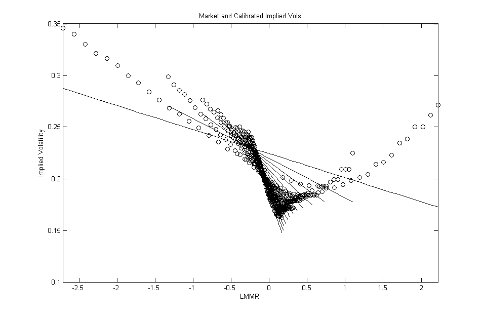
Figure 2: Market (circles) and calibrated (solid lines) implied volatilities for options on crude-oil futures with maturity greater than 90 days.

Figure 3: Market (circles) and calibrated (solid lines) implied volatilities for options on crude-oil futures using all data available.

5 Comparison to Previous Work

Multiscale stochastic volatility models were considered in the context of mean reverting asset price in the papers Hikspoors and Jaimungal (2008) and Chiu et al. (2011). Both derived the first-order approximation of options on the spot price. However, only Hikspoors and Jaimungal (2008) handled options on futures. Therefore, we will focus this section on this work.

In Hikspoors and Jaimungal (2008), the authors have applied the method first developed in Cotton et al. (2004) to approximate the price of options on commodity futures. This method consists of writing the payoff function as its first-order Taylor polynomial around the zero-order term of the future price expansion (3.1) and then applying the singular-perturbation arguments introduced by Fouque et al. to finally derive the approximation. Another aspect of their method that is fundamentally different of ours is that they consider the variable of interest to be the spot price of the commodity, denoted here by $V_{t}$, while we consider the future prices of $V$, denoted here by $F_{t,T}$. As we will see below, this is one of the reasons no simple calibration procedure can be designed using their first-order approximation.

The authors present two classes of models: one-factor and two-factor models. Both models share one common aspect: the commodity presents fast-mean reversion stochastic volatility. Our model (2.8) is thus an extension of their one-factor model, where we have added the slow time-scale to the stochastic volatility dynamics. However, compared to Hikspoors and Jaimungal (2008), the main contributions of our work are:

• we do not rely on the Taylor expansion of the payoff function to derive the first-order approximation of options prices and therefore no additional smoothness assumption is necessary. The inversion argument presented in Section 3.4 allows us to overcome this smoothness restriction to the payoff function;

• our first-order correction (see Summary 3.6 for instance) is a substantial betterment of theirs, because it involves only Greeks of the zero-order term. Their first-order correction presents a complicated term that involves the expectation:

  $$\mathbb{E}_{\mathbb{Q}}[h_{0}(T_{0},\overline{U}_{T_{0}})\varphi^{\prime}(h_{0}(T_{0},\overline{U}_{T_{0}}))\ |\ \overline{U}_{t}=u],$$

  where we are using the notation established in the previous sections and $\overline{U}$ is the process $U$ of Equation (2.8) with $\eta(y,z)=\bar{\eta}(z)$;

• we present a simple calibration procedure of the market group parameters. The simple expression of our first-order correction is one of the reasons such calibration procedure is possible. However, the essential aspect of our method that is the cornerstone of the procedure is that we consider the future price $F_{t,T}$ as the variable, and not spot price $V_{t}$. So, since the future price is a martingale (as opposed to the $V$), better formulas for the Greeks of the 0-order term are available. Mainly, Equation (4.3) holds true.

6 Concluding Remarks and Future Directions

We have presented a general method to derive the first-order approximation of compound derivatives and developed it thoroughly in the case of derivatives on future contracts. Although the method may seem to be involved, it does not require any additional hypothesis on the regularity of the payoff function other than the ones inherent to the perturbation theory. Moreover, we presented a calibration procedure associated with the method, for which we derive formulas for the market group parameters. A practical numerical example of the calibration procedure is given using data of Black implied volatilities of options on crude-oil futures.

One direction for further study would be to connect the model and asymptotic expansions proposed in this work with the celebrated Schwartz-Smith Schwartz and Smith (2000) and Gibson-Schwartz Gibson and Schwartz (1990) models for commodity prices. In particular, an important question would be the computation of the risk premium as in Gibson and Schwartz (1990).

Appendix A PDE Expansion

Formally write, for $k=1,2,3$,

$$\psi^{\varepsilon,\delta}_{k}(t,x,y,z,T)=\sum_{i,j\geq 0}(\sqrt{\varepsilon})^{i}(\sqrt{\delta})^{j}\psi_{k,i,j}(t,x,y,z,T).$$

In what follows we will compute only the terms of the above expansion that are necessary for the computation of the first-order approximation of derivatives on $F_{t,T}$.

A.1 Expanding $\psi_{1}^{\varepsilon,\delta}$

By the chain rule

$$\psi^{\varepsilon,\delta}_{1}(t,x,y,z,T)=\frac{1}{\displaystyle\frac{\partial H}{\partial x}^{\varepsilon,\delta}(t,x,y,z,T)},$$

and then one can easily see that

$$\psi_{1,0,0}(t,x,y,z,T)=\frac{1}{\displaystyle\frac{\partial H_{0}}{\partial x}(t,x,z,T)}=\frac{\partial h_{0}}{\partial u}(t,H_{0}(t,x,z,T),z,T).$$

Since

$$\frac{\partial h_{0}}{\partial u}(t,u,z,T)=e^{-\kappa(T-t)}h_{0}(t,u,z,T),$$

we have the following formula for $\psi_{1,0,0}$:

(A.1) $$\psi_{1,0,0}(t,x,T)=e^{-\kappa(T-t)}h_{0}(t,H_{0}(t,x,z,T),z,T)=e^{-\kappa(T-t)}x.$$

Moreover, by Lemma 3.1,

$$H_{1,0}(t,x,z,T) =-\frac{h_{1,0}(t,H_{0}(t,x,z,T),z,T)}{\displaystyle\frac{\partial h_{0}}{\partial u}(t,H_{0}(t,x,z,T),z,T)}$$

$$=-\frac{g(t,T)V_{3}(z)e^{-3\kappa(T-t)}x}{e^{-\kappa(T-t)}x}=-g(t,T)V_{3}(z)e^{-2\kappa(T-t)},$$

which is independent of $x$, and therefore,

(A.2) $$\psi_{1,1,0}(t,x,z,T)=-\frac{1}{\displaystyle\left(\frac{\partial H_{0}}{\partial x}(t,x,z,T)\right)^{2}}\frac{\partial H_{1,0}}{\partial x}(t,x,z,T)=0.$$

We also have

(A.3) $$\psi_{1,0,1}(t,x,z,T)=0.$$

A.2 Expanding $\psi_{2}^{\varepsilon,\delta}$

Recall that the first four terms of the expansion of $h^{\varepsilon,\delta}$ do not depend on $y$. Thus

(A.4) $$\psi_{2,0,0}=\psi_{2,0,1}=\psi_{2,1,0}=\psi_{2,1,1}=0.$$

Furthermore, again by the chain rule, we have

$$\psi_{2}^{\varepsilon,\delta}(t,x,y,z,T)=-\psi_{1}^{\varepsilon,\delta}(t,x,y,z,T)\frac{\partial H}{\partial y}^{\varepsilon,\delta}(t,x,y,z,T).$$

From this, we get

$$\psi_{2,2,0}(t,x,y,z,T) =-\psi_{1,0,0}(t,x,T)\frac{\partial H_{2,0}}{\partial y}(t,x,y,z,T)$$

$$=-e^{-\kappa(T-t)}x\frac{\partial H_{2,0}}{\partial y}(t,x,y,z,T).$$

In order to compute $H_{2,0}$ we need to go further in the expansions of $h^{\varepsilon,\delta}$ and $H^{\varepsilon,\delta}$. One can compute the term of order $(2,0)$ in $H^{\varepsilon,\delta}$ and then conclude

$$H_{2,0}(t,x,y,z,T) =-\frac{h_{2,0}(t,H_{0}(t,x,z,T),y,z,T)}{\frac{\partial h_{0}}{\partial u}(t,H_{0}(t,x,z,T),z,T)}$$

$$-\frac{1}{2}\frac{\frac{\partial^{2}h_{0}}{\partial^{2}u}(t,H_{0}(t,x,z,T),z,T)}{\frac{\partial h_{0}}{\partial u}(t,H_{0}(t,x,z,T),z,T)}H_{1,0}^{2}(t,x,z,T)$$

$$-\frac{\frac{\partial h_{1,0}}{\partial u}(t,H_{0}(t,x,z,T),z,T)}{\frac{\partial h_{0}}{\partial u}(t,H_{0}(t,x,z,T),z,T)}H_{1,0}(t,x,z,T),$$

which implies

$$\frac{\partial H_{2,0}}{\partial y}(t,x,y,z,T)=-\frac{\frac{\partial h_{2,0}}{\partial y}(t,H_{0}(t,x,z,T),y,z,T)}{\frac{\partial h_{0}}{\partial u}(t,H_{0}(t,x,z,T),z,T)}.$$

From (3.10), we know that

$$\frac{\partial h_{2,0}}{\partial y}(t,u,y,z,T) =-\frac{1}{2}\frac{\partial\phi}{\partial y}(y,z)\frac{\partial^{2}h_{0}}{\partial u^{2}}(t,u,z,T)$$

$$=-\frac{1}{2}e^{-2\kappa(T-t)}\frac{\partial\phi}{\partial y}(y,z)h_{0}(t,u,z,T),$$

and hence

$$\frac{\partial H_{2,0}}{\partial y}(t,x,y,z,T)=\frac{\frac{1}{2}e^{-2\kappa(T-t)}\frac{\partial\phi}{\partial y}(y,z)x}{e^{-\kappa(T-t)}x}=\frac{1}{2}e^{-\kappa(T-t)}\frac{\partial\phi}{\partial y}(y,z).$$

Finally, this gives the formula

(A.5) $$\psi_{2,2,0}(t,x,y,z,T)=-\frac{1}{2}e^{-2\kappa(T-t)}\frac{\partial\phi}{\partial y}(y,z)x.$$

A.3 Expanding $\psi_{3}^{\varepsilon,\delta}$

By the chain rule, we have

$$\psi_{3}^{\varepsilon,\delta}(t,x,y,z,T)=-\psi_{1}^{\varepsilon,\delta}(t,x,y,z,T)\frac{\partial H}{\partial z}^{\varepsilon,\delta}(t,x,y,z,T),$$

and then

(A.6) $$\psi_{3,0,0}(t,x,z) =-\psi_{1,0,0}(t,x,T)\frac{\partial H_{0}}{\partial z}(t,x,y,z,T)$$

$$=\frac{\partial h_{0}}{\partial z}(t,H_{0}(t,x,z,T),z,T)$$

$$=\frac{1}{2\kappa}\bar{\eta}(z)\bar{\eta}^{\prime}(z)(1-e^{-2\kappa(T-t)})x.$$

A.4 An Expansion of the Pricing PDE

Define

$$\Psi_{n,p}^{k,m}(t,x,y,z,T)=\sum_{i=0}^{n}\sum_{j=0}^{p}\psi_{k,i,j}(t,x,y,z,T)\psi_{m,n-i,p-j}(t,x,y,z,T),$$

which is the $(n,p)$-order coefficient of the formal power series of $\psi^{\varepsilon,\delta}_{k}\psi^{\varepsilon,\delta}_{m}$:

$$\psi^{\varepsilon,\delta}_{k}(t,x,y,z,T)\psi^{\varepsilon,\delta}_{m}(t,x,y,z,T)$$

$$=\sum_{i,j,l,r\geq 0}(\sqrt{\varepsilon})^{l+i}(\sqrt{\delta})^{j+r}\psi_{k,i,j}(t,x,y,z,T)\psi_{m,l,r}(t,x,y,z,T)$$

$$=\sum_{n,p\geq 0}(\sqrt{\varepsilon})^{n}(\sqrt{\delta})^{p}\left(\sum_{i=0}^{n}\sum_{j=0}^{p}\psi_{k,i,j}(t,x,y,z,T)\psi_{m,n-i,p-j}(t,x,y,z,T)\right).$$

Therefore, we have the following formal expansion for the operator $\mathcal{L}^{\varepsilon,\delta}$ where we drop the variables $(t,x,y,z,T)$ for simplicity,

$$\mathcal{L}^{\varepsilon,\delta}= \frac{1}{\varepsilon}\left(\mathcal{L}_{0}+\frac{1}{2}\Psi^{2,2}_{0}\beta^{2}(y)\frac{\partial^{2}}{\partial x^{2}}+\psi_{2,0,0}\beta^{2}(y)\frac{\partial^{2}}{\partial x\partial y}\right)$$

$$+ \frac{1}{\sqrt{\varepsilon}}\left(\raisebox{1.5pt}{$\rho$}_{1}\Psi^{1,2}_{0}\eta(y,z)\beta(y)\frac{\partial^{2}}{\partial x^{2}}+\raisebox{1.5pt}{$\rho$}_{1}\psi_{1,0,0}\eta(y,z)\beta(y)\frac{\partial^{2}}{\partial x\partial y}\right.$$

$$+ \left.\frac{1}{2}\Psi^{2,2}_{1,0}\beta^{2}(y)\frac{\partial^{2}}{\partial x^{2}}+\psi_{2,1,0}\beta^{2}(y)\frac{\partial^{2}}{\partial x\partial y}\right)$$

$$+ \left(\frac{\partial}{\partial t}+\frac{1}{2}\Psi^{1,1}_{0}\eta^{2}(y,z)\frac{\partial^{2}}{\partial x^{2}}-r\cdot+\raisebox{1.5pt}{$\rho$}_{1}\Psi^{1,2}_{1,0}\eta(y,z)\beta(y)\frac{\partial^{2}}{\partial x^{2}}\right.$$

$$+ \left.\raisebox{1.5pt}{$\rho$}_{1}\psi_{1,1,0}\eta(y,z)\beta(y)\frac{\partial^{2}}{\partial x\partial y}+\frac{1}{2}\Psi^{2,2}_{2,0}\beta^{2}(y)\frac{\partial^{2}}{\partial x^{2}}+\psi_{2,2,0}\beta^{2}(y)\frac{\partial^{2}}{\partial x\partial y}\right)$$

$$+ \sqrt{\varepsilon}\left(\frac{1}{2}\Psi^{2,2}_{3,0}\beta^{2}(y)\frac{\partial^{2}}{\partial x^{2}}+\psi_{2,3,0}\beta^{2}(y)\frac{\partial^{2}}{\partial x\partial y}+\raisebox{1.5pt}{$\rho$}_{1}\Psi_{2,0}^{1,2}\eta(y,z)\beta(y)\frac{\partial^{2}}{\partial x^{2}}\right.$$

$$+ \left.\raisebox{1.5pt}{$\rho$}_{1}\psi_{1,2,0}\eta(y,z)\beta(y)\frac{\partial^{2}}{\partial x\partial y}+\frac{1}{2}\Psi^{1,1}_{1,0}\beta^{2}(y)\frac{\partial^{2}}{\partial x^{2}}\right)$$

$$+ \sqrt{\delta}\left(\raisebox{1.5pt}{$\rho$}_{2}\Psi^{1,3}_{0}\eta(y,z)g(z)\frac{\partial^{2}}{\partial x^{2}}+\raisebox{1.5pt}{$\rho$}_{2}\psi_{1,0,0}\eta(y,z)g(z)\frac{\partial^{2}}{\partial x\partial z}\right.$$

$$+ \frac{1}{2}\Psi^{2,2}_{2,1}\beta^{2}(y)\frac{\partial^{2}}{\partial x^{2}}+\psi_{2,2,1}\beta^{2}(y)\frac{\partial^{2}}{\partial x\partial y}$$

$$+ \left.\raisebox{1.5pt}{$\rho$}_{2}\Psi^{1,2}_{1,1}\eta(y,z)\beta(y)\frac{\partial^{2}}{\partial x^{2}}+\raisebox{1.5pt}{$\rho$}_{2}\psi_{1,1,1}\eta(y,z)\beta(y)\frac{\partial^{2}}{\partial x\partial y}+\frac{1}{2}\Psi^{1,1}_{0,1}\eta^{2}(y,z)\frac{\partial^{2}}{\partial x^{2}}\right)$$

$$+ \sqrt{\frac{\delta}{\varepsilon}}\left(\raisebox{1.5pt}{$\rho$}_{12}\Psi^{2,3}_{0}\beta(y)g(z)\frac{\partial^{2}}{\partial x^{2}}+\raisebox{1.5pt}{$\rho$}_{12}\psi_{3,0,0}\beta(y)g(z)\frac{\partial^{2}}{\partial x\partial y}\right.$$

$$+ \raisebox{1.5pt}{$\rho$}_{12}\psi_{2,0,0}\beta(y)g(z)\frac{\partial^{2}}{\partial x\partial z}+\raisebox{1.5pt}{$\rho$}_{12}\beta(y)g(z)\frac{\partial^{2}}{\partial y\partial z}+\frac{1}{2}\Psi^{2,2}_{1,1}\beta^{2}(y)\frac{\partial^{2}}{\partial x^{2}}$$

$$+ \left.\psi_{2,1,1}\beta^{2}(y)\frac{\partial^{2}}{\partial x\partial y}+\raisebox{1.5pt}{$\rho$}_{1}\Psi^{1,2}_{0,1}\eta(y,z)\beta(y)\frac{\partial^{2}}{\partial x^{2}}+\raisebox{1.5pt}{$\rho$}_{1}\psi_{1,0,1}\eta(y,z)\beta(y)\frac{\partial^{2}}{\partial x\partial y}\right).$$

$$+ \mathcal{L}^{\varepsilon,\delta}_{R}.$$

Then we write, with obvious notation,

$$\mathcal{L}^{\varepsilon,\delta}=\frac{1}{\varepsilon}\mathcal{D}_{-2,0}+\frac{1}{\sqrt{\varepsilon}}\mathcal{D}_{-1,0}+\mathcal{D}_{0,0}+\sqrt{\varepsilon}\mathcal{D}_{1,0}+\sqrt{\delta}\mathcal{D}_{0,1}+\sqrt{\frac{\delta}{\varepsilon}}\mathcal{D}_{-1,1}+\mathcal{L}^{\varepsilon,\delta}_{R}.$$

In order to simplify the operators $\mathcal{D}_{i,j}$, note that $\Psi^{2,k}_{0}=0$, for $k=1,2,3$,

$$\Psi^{2,2}_{1,0}=\Psi^{2,2}_{0,1}=\Psi^{1,2}_{1,0}=\Psi^{2,2}_{2,0}=\Psi^{2,2}_{3,0}=\Psi_{2,1}^{2,2}=\Psi_{1,1}^{1,2}=0,$$

and $\Psi^{1,1}_{1,0}=\Psi^{1,1}_{0,1}=0$. Hence,

$$\bullet\mathcal{D}_{-2,0}=\mathcal{L}_{0}+\frac{1}{2}\cancelto{\scriptstyle 0}{\Psi^{2,2}_{0}}\beta^{2}(y)\frac{\partial^{2}}{\partial x^{2}}+\cancelto{\scriptstyle 0}{\psi_{2,0,0}}\beta^{2}(y)\frac{\partial^{2}}{\partial x\partial y}=\mathcal{L}_{0}$$

$$\bullet\mathcal{D}_{-1,0}=\raisebox{1.5pt}{$\rho$}_{1}\cancelto{\scriptstyle 0}{\Psi^{1,2}_{0}}\eta(y,z)\beta(y)\frac{\partial^{2}}{\partial x^{2}}+\raisebox{1.5pt}{$\rho$}_{1}\psi_{1,0,0}\eta(y,z)\beta(y)\frac{\partial^{2}}{\partial x\partial y}$$

$$+\frac{1}{2}\cancelto{\scriptstyle 0}{\Psi^{2,2}_{1,0}}\beta^{2}(y)\frac{\partial^{2}}{\partial x^{2}}+\cancelto{\scriptstyle 0}{\psi_{2,1,0}}\beta^{2}(y)\frac{\partial^{2}}{\partial x\partial y}=\raisebox{1.5pt}{$\rho$}_{1}\psi_{1,0,0}\eta(y,z)\beta(y)\frac{\partial^{2}}{\partial x\partial y}$$

$$\bullet\mathcal{D}_{0,0}=\frac{\partial}{\partial t}+\frac{1}{2}\Psi^{1,1}_{0}\eta^{2}(y,z)\frac{\partial^{2}}{\partial x^{2}}-r\cdot+\raisebox{1.5pt}{$\rho$}_{1}\cancelto{\scriptstyle 0}{\Psi^{1,2}_{1,0}}\eta(y,z)\beta(y)\frac{\partial^{2}}{\partial x^{2}}$$

$$+\raisebox{1.5pt}{$\rho$}_{1}\cancelto{\scriptstyle 0}{\psi_{1,1,0}}\eta(y,z)\beta(y)\frac{\partial^{2}}{\partial x\partial y}++\frac{1}{2}\cancelto{\scriptstyle 0}{\Psi^{2,2}_{2,0}}\beta^{2}(y)\frac{\partial^{2}}{\partial x^{2}}+\psi_{2,2,0}\beta^{2}(y)\frac{\partial^{2}}{\partial x\partial y}$$

$$=\frac{\partial}{\partial t}+\frac{1}{2}\psi_{1,0,0}^{2}\eta^{2}(y,z)\frac{\partial^{2}}{\partial x^{2}}-r\cdot+\psi_{2,2,0}\beta^{2}(y)\frac{\partial^{2}}{\partial x\partial y}$$

$$\bullet\mathcal{D}_{1,0}=\frac{1}{2}\cancelto{\scriptstyle 0}{\Psi^{2,2}_{3,0}}\beta^{2}(y)\frac{\partial^{2}}{\partial x^{2}}+\psi_{2,3,0}\beta^{2}(y)\frac{\partial^{2}}{\partial x\partial y}+\raisebox{1.5pt}{$\rho$}_{1}\cancelto{\scriptstyle\psi_{1,0,0}\psi_{2,2,0}}{\Psi_{2,0}^{1,2}}\eta(y,z)\beta(y)\frac{\partial^{2}}{\partial x^{2}}$$

$$+\raisebox{1.5pt}{$\rho$}_{1}\psi_{1,2,0}\eta(y,z)\beta(y)\frac{\partial^{2}}{\partial x\partial y}+\frac{1}{2}\cancelto{\scriptstyle 0}{\Psi^{1,1}_{1,0}}\beta^{2}(y)\frac{\partial^{2}}{\partial x^{2}}$$

$$=\left(\psi_{2,3,0}\beta^{2}(y)+\raisebox{1.5pt}{$\rho$}_{1}\psi_{1,2,0}\eta(y,z)\beta(y)\right)\frac{\partial^{2}}{\partial x\partial y}+\raisebox{1.5pt}{$\rho$}_{1}\psi_{1,0,0}\psi_{2,2,0}\eta(y,z)\beta(y)\frac{\partial^{2}}{\partial x^{2}}$$

$$\bullet\mathcal{D}_{0,1}=\raisebox{1.5pt}{$\rho$}_{2}\Psi^{1,3}_{0}\eta(y,z)g(z)\frac{\partial^{2}}{\partial x^{2}}+\raisebox{1.5pt}{$\rho$}_{2}\psi_{1,0,0}\eta(y,z)g(z)\frac{\partial^{2}}{\partial x\partial z}+\frac{1}{2}\cancelto{\scriptstyle 0}{\Psi^{2,2}_{2,1}}\beta^{2}(y)\frac{\partial^{2}}{\partial x^{2}}$$

$$+\psi_{2,2,1}\beta^{2}(y)\frac{\partial^{2}}{\partial x\partial y}+\raisebox{1.5pt}{$\rho$}_{2}\cancelto{\scriptstyle 0}{\Psi^{1,2}_{1,1}}\eta(y,z)\beta(y)\frac{\partial^{2}}{\partial x^{2}}+\raisebox{1.5pt}{$\rho$}_{2}\psi_{1,1,1}\eta(y,z)\beta(y)\frac{\partial^{2}}{\partial x\partial y}$$

$$+\frac{1}{2}\cancelto{\scriptstyle 0}{\Psi^{1,1}_{0,1}}\eta^{2}(y,z)\frac{\partial^{2}}{\partial x^{2}}=(\raisebox{1.5pt}{$\rho$}_{2}\psi_{1,0,0}\psi_{3,0,0}\eta(y,z)g(z))\frac{\partial^{2}}{\partial x^{2}}$$

$$+\raisebox{1.5pt}{$\rho$}_{2}\psi_{1,0,0}\eta(y,z)g(z)\frac{\partial^{2}}{\partial x\partial z}+(\psi_{2,2,1}\beta^{2}(y)+\raisebox{1.5pt}{$\rho$}_{2}\psi_{1,1,1}\eta(y,z)\beta(y))\frac{\partial^{2}}{\partial x\partial y}$$

$$\bullet\mathcal{D}_{-1,1}=\raisebox{1.5pt}{$\rho$}_{12}\cancelto{\scriptstyle 0}{\Psi^{2,3}_{0}}\beta(y)g(z)\frac{\partial^{2}}{\partial x^{2}}+\raisebox{1.5pt}{$\rho$}_{23}\psi_{3,0,0}\beta(y)g(z)\frac{\partial^{2}}{\partial x\partial y}$$

$$+\raisebox{1.5pt}{$\rho$}_{12}\cancelto{\scriptstyle 0}{\psi_{2,0,0}}\beta(y)g(z)\frac{\partial^{2}}{\partial x\partial z}+\raisebox{1.5pt}{$\rho$}_{12}\beta(y)g(z)\frac{\partial^{2}}{\partial y\partial z}+\frac{1}{2}\cancelto{\scriptstyle 0}{\Psi^{2,2}_{1,1}}\beta^{2}(y)\frac{\partial^{2}}{\partial x^{2}}$$

$$+\cancelto{\scriptstyle 0}{\psi_{2,1,1}}\beta^{2}(y)\frac{\partial^{2}}{\partial x\partial y}+\raisebox{1.5pt}{$\rho$}_{1}\cancelto{\scriptstyle 0}{\Psi^{1,2}_{0,1}}\eta(y,z)\beta(y)\frac{\partial^{2}}{\partial x^{2}}$$

$$+\raisebox{1.5pt}{$\rho$}_{1}\cancelto{\scriptstyle 0}{\psi_{1,0,1}}\eta(y,z)\beta(y)\frac{\partial^{2}}{\partial x\partial y}=\raisebox{1.5pt}{$\rho$}_{12}\psi_{3,0,0}\beta(y)g(z)\frac{\partial^{2}}{\partial x\partial y}+\raisebox{1.5pt}{$\rho$}_{12}\beta(y)g(z)\frac{\partial^{2}}{\partial y\partial z}$$

It is clear from the above choices that the coefficients of the operator $\mathcal{L}^{\varepsilon,\delta}_{R}$ are of order $(\varepsilon+\delta)$. Hence, if $f$ is smooth and bounded with all derivatives bounded,

(A.7) $$\mathcal{L}^{\varepsilon,\delta}_{R}f(t,x,y,z)=O(\varepsilon+\delta).$$

Appendix B Proof of Theorem 3.2

By the regularization argument presented in Fouque et al. (2003a), extended for the addition of the slow factor Fouque et al. (2011), we may assume that the payoff $\varphi$ is smooth and bounded with bounded derivatives. Additionally, in the reference mentioned above, the authors outlined an argument to improve the error bound from $O(\varepsilon\log|\varepsilon|+\delta)$ to $O(\varepsilon+\delta)$.

Following the proof of Theorem 4.10 given in Fouque et al. (2011) for the Equity case, we go further in the approximation of $P^{\varepsilon,\delta}$ and define the higher-order approximation:

(B.1) $$\widehat{P}^{\varepsilon,\delta}=\widetilde{P}^{\varepsilon,\delta}+\varepsilon(P_{2,0}+\sqrt{\varepsilon}P_{3,0})+\sqrt{\delta}(\sqrt{\varepsilon}P_{1,1}+\varepsilon P_{2,1}),$$

and moreover, we introduce

(B.2) $$\widehat{\mathcal{L}}^{\varepsilon,\delta}=\frac{1}{\varepsilon}\mathcal{L}_{0}+\frac{1}{\sqrt{\varepsilon}}\mathcal{L}_{1}+\mathcal{L}_{2}+\sqrt{\varepsilon}\mathcal{L}_{3}+\sqrt{\delta}\mathcal{M}_{1}+\sqrt{\frac{\delta}{\varepsilon}}\mathcal{M}_{3}.$$

Necessary properties of the additional terms in the expansion (B.1) can be derived in the same way as it is done in Fouque et al. (2011) and thus we skip the details here. Next, we define the residual

(B.3) $$R^{\varepsilon,\delta}=P^{\varepsilon,\delta}-\widehat{P}^{\varepsilon,\delta}$$

and use the pricing PDE (3.21) to conclude that

$$\mathcal{L}^{\varepsilon,\delta}R^{\varepsilon,\delta} =\mathcal{L}^{\varepsilon,\delta}(P^{\varepsilon,\delta}-\widehat{P}^{\varepsilon,\delta})=-\mathcal{L}^{\varepsilon,\delta}\widehat{P}^{\varepsilon,\delta}$$

$$=-(\widehat{\mathcal{L}}^{\varepsilon,\delta}+\mathcal{L}^{\varepsilon,\delta}_{R})\widehat{P}^{\varepsilon,\delta}=-\widehat{\mathcal{L}}^{\varepsilon,\delta}\widehat{P}^{\varepsilon,\delta}-\mathcal{L}^{\varepsilon,\delta}_{R}\widehat{P}^{\varepsilon,\delta}.$$

Hence, mimicking the computations from Fouque et al. (2011), we can write

$$\widehat{\mathcal{L}}^{\varepsilon,\delta}\widehat{P}^{\varepsilon,\delta}=\varepsilon R_{1}^{\varepsilon}+\sqrt{\varepsilon\delta}R_{2}^{\varepsilon}+\delta R_{3}^{\varepsilon},$$

where $R_{1}^{\varepsilon}$, $R_{2}^{\varepsilon}$ and $R_{3}^{\varepsilon}$ can be exactly computed as linear combinations of $\mathcal{L}_{k}P_{i,j}$ and $\mathcal{M}_{l}P_{i,j}$, for some $k,l,i,j$. However, the important fact about $R_{i}^{\varepsilon}$ is that they are smooth functions of $t,x,y,z$, for small $\varepsilon$ and $\delta$, bounded by smooth functions of $t,x,y,z$ independent of $\varepsilon$ and $\delta$, uniformly bounded in $t,x,z$ and at most linearly growing in $y$. Additionally, from (A.7), we can define $R_{4}^{\varepsilon}$ and conclude that

$$R_{4}^{\varepsilon}=\mathcal{L}^{\varepsilon,\delta}_{R}\widehat{P}^{\varepsilon,\delta}=O(\varepsilon+\delta),$$

since $\widehat{P}^{\varepsilon,\delta}$ is bounded and smooth with all derivatives bounded. This follows from the same arguments presented in proof of Theorem 4.10 of Fouque et al. (2011) with some minor differences to include $\mathcal{L}_{3}$. Therefore, the residual $R^{\varepsilon,\delta}$ solves the PDE

(B.8) $$\left\{\begin{array}[]{l}\mathcal{L}^{\varepsilon,\delta}R^{\varepsilon,\delta}+\varepsilon R_{1}^{\varepsilon}+\sqrt{\varepsilon\delta}R_{2}^{\varepsilon}+\delta R_{3}^{\varepsilon}+R_{4}^{\varepsilon}=0,\\ \\ R^{\varepsilon,\delta}(T_{0},x,y,z,T)=-\varepsilon(P_{2,0}+\sqrt{\varepsilon}P_{3,0})(T_{0},x,y,z,T)\\ \hskip 79.6678pt-\sqrt{\varepsilon\delta}(P_{1,1}+\sqrt{\varepsilon}P_{2,1})(T_{0},x,y,z,T),\end{array}\right.$$

and then all the computations regarding the Feynman-Kac probabilistic representation of $R^{\varepsilon,\delta}$ and the growth control of the source and final condition can be carried out just as in Fouque et al. (2011) in order to conclude that $R^{\varepsilon,\delta}=O(\varepsilon+\delta)$. Lastly, the desired result follows because

$$|P^{\varepsilon,\delta}-\widetilde{P}^{\varepsilon,\delta}|\leq|R^{\varepsilon,\delta}|+|\widehat{P}^{\varepsilon,\delta}-\widetilde{P}^{\varepsilon,\delta}|.$$

∎

Appendix C Computing $P_{0,1}^{\delta}$ explicitly for European derivatives

Let us write $P^{\delta}_{0,1}$ in terms of Greeks of $P_{B}$ by solving the PDE (3.60). Note first that

$$\frac{\partial P_{0}}{\partial z}(t,x,z,T)=\frac{\partial P_{B}}{\partial\sigma}(t,x,\bar{\sigma}_{t,T_{0}}(z,T))\frac{\partial\bar{\sigma}_{t,T_{0}}}{\partial z}(z,T).$$

Since $P_{B}$ satisfies the Black equation and the European derivative has maturity $T_{0}$, we have the relation between the Vega and the Gamma:

$$\frac{\partial P_{B}}{\partial\sigma}(t,x,\sigma)=(T_{0}-t)\sigma D_{2}P_{B}(t,x,\sigma).$$

Moreover,

$$\frac{\partial\bar{\sigma}_{t,T_{0}}}{\partial z}(z,T)=\bar{\eta}^{\prime}(z)\lambda_{\sigma}(t,T_{0},T,\kappa).$$

Combining the above equations, we obtain

$$-f_{0}(t,T)\mathcal{A}_{0}^{\delta}P_{0}-f_{1}(t,T)\mathcal{A}_{1}^{\delta}P_{0}$$

$$=-f_{0}(t,T)\mathcal{A}_{0}^{\delta}P_{0}-f_{1}(t,T)V_{1}^{\delta}(z)(T_{0}-t)\bar{\eta}(z)\bar{\eta}^{\prime}(z)\lambda^{2}_{\sigma}(t,T_{0},T,\kappa)D_{1}D_{2}P_{0}$$

$$=-f_{0}(t,T)\mathcal{A}_{0}^{\delta}P_{0}-\tilde{f}_{1}(t,T)\mathcal{A}_{0}^{\delta}D_{1}P_{0},$$

where

$$\tilde{f}_{1}(t,T)=f_{1}(t,T)(e^{-2\kappa(T-T_{0})}-e^{-2\kappa(T-t)}).$$

Hence, we deduce the following PDE for $P_{0,1}^{\delta}$:

(C.4) $$\left\{\begin{array}[]{l}\mathcal{L}_{B}(\bar{\sigma}(t,z,T))P^{\delta}_{0,1}=-f_{0}(t,T)\mathcal{A}_{0}^{\delta}P_{0}-\tilde{f}_{1}(t,T)\mathcal{A}_{0}^{\delta}D_{1}P_{0},\\ \\ P^{\delta}_{0,1}(T_{0},x,z,T)=0.\end{array}\right.$$

By the same argument used to deduce Equation (3.52), and using the linearity of the differential operators involved, we can easily conclude

$$P^{\delta}_{0,1}(t,x,z,T)=\left(\int_{t}^{T_{0}}f_{0}(u,T)du\right)\mathcal{A}_{0}^{\delta}P_{0}+\left(\int_{t}^{T_{0}}\tilde{f}_{1}(u,T)du\right)\mathcal{A}_{0}^{\delta}D_{1}P_{0}.$$

Computing these integrals gives us the formulas

(C.5) $$\lambda_{0}(t,T_{0},T,\kappa)=\frac{1}{T_{0}-t}\int_{t}^{T_{0}}f_{0}(u,T)du$$

$$=\frac{e^{-\kappa(T-T_{0})}-e^{-\kappa(T-t)}}{\kappa(T_{0}-t)}-\frac{e^{-3\kappa(T-T_{0})}-e^{-3\kappa(T-t)}}{3\kappa(T_{0}-t)}$$

$$=\lambda(t,T_{0},T,\kappa)-\lambda(t,T_{0},T,3\kappa),$$

(C.6) $$\lambda_{1}(t,T_{0},T,\kappa)=\frac{1}{T_{0}-t}\int_{t}^{T_{0}}\tilde{f}_{1}(u,T)du$$

$$=e^{-2\kappa(T-T_{0})}\frac{e^{-\kappa(T-T_{0})}-e^{-\kappa(T-t)}}{\kappa(T_{0}-t)}-\frac{e^{-3\kappa(T-T_{0})}-e^{-3\kappa(T-t)}}{3\kappa(T_{0}-t)}$$

$$=e^{-2\kappa(T-T_{0})}\lambda(t,T_{0},T,\kappa)-\lambda(t,T_{0},T,3\kappa).$$

References

- Chiu et al. (2011) M. C. Chiu, Y. Wai Lo, and H.Y. Wong. Asymptotic Expansion for Pricing Options on Mean-Reverting Assets with Multiscale Stochastic Volatility. Operations Research Letters, 39:289–295, 2011.
- Cotton et al. (2004) P. Cotton, J.-P. Fouque, G. Papanicolaou, and R. Sircar. Stochastic Volatility Corrections for Interest Rate Derivatives. Mathematical Finance, 14:173–200, 2004.
- Delbaen and Schachermayer (2008) F. Delbaen and W. Schachermayer. The Mathematics of Arbitrage. Springer Finance, 2008.
- Dupire (2009) B. Dupire. Functional Itô Calculus. SSRN, 2009. URL http://ssrn.com/abstract=1435551.
- Fouque and Han (2005) J.-P. Fouque and C.H. Han. Evaluation of Compound Options Using Perturbation Approximation. Journal of Computational Finance, 9:41–61, 2005.
- Fouque et al. (2003a) J.-P. Fouque, G. Papanicolaou, R. Sircar, and K. Sølna. Singular Pertubations in Option Pricing. SIAM Journal on Applied Mathematics, 63:1648–65, 2003a.
- Fouque et al. (2003b) J.-P. Fouque, G. Papanicolaou, R. Sircar, and K. Sølna. Short Time-scale in S&P 500 Volatility. Journal of Computational Finance, 6:1–23, 2003b.
- Fouque et al. (2004) J.-P. Fouque, G. Papanicolaou, R. Sircar, and K. Sølna. Maturity Cycles in Implied Volatility. Finance & Stochastics, 8(4):451–477, 2004.
- Fouque et al. (2011) J.-P. Fouque, G. Papanicolaou, R. Sircar, and K. Sølna. Multiscale Stochastic Volatility for Equity, Interest Rate, And Credit Derivatives. Cambridge University Press, 2011.
- Fouque et al. (2012) J.-P. Fouque, M. Lorig, and R. Sircar. Second Order Multiscale Stochastic Volatility Asymptotics: Stochastic Terminal Layer Analysis & Calibration. Submitted, 2012.
- Gatheral (2006) J. Gatheral. The Volatility Surface - A Practitioner’s Guide. Wiley, 2006.
- Gibson and Schwartz (1990) R. Gibson and E.S. Schwartz. Stochastic Convenience Yield and the Pricing of Oil Contingent Claims. Journal of Finance, pages 959–976, 1990.
- Hikspoors and Jaimungal (2008) S. Hikspoors and S. Jaimungal. Asymptotic Pricing of Commodity derivatives for Stochastic Volatility Spot Models. Applied Mathematical Finance, 15:449–447, 2008.
- Musiela and Rutkowski (2008) M. Musiela and M. Rutkowski. Martingale Methods in Financial Modelling. Springer, Second edition, 2008.
- Schwartz (1997) E. S. Schwartz. The Stochastic Behavior of Commodity Prices: Implications for Valuation and Hedging. Journal of Finance, 52:923–973, 1997.
- Schwartz and Smith (2000) E. S. Schwartz and J.E. Smith. Short-Term Variations and Long-Term Dynamics in Commodity Prices. Management Science, 46:893–911, 2000.