Abstract

In this paper, we consider the discrete deformation of the discrete space curves with constant torsion described by the discrete mKdV or the discrete sine-Gordon equations, and show that it is formulated as the torsion-preserving equidistant deformation on the osculating plane which satisfies the isoperimetric condition. The curve is reconstructed from the deformation data by using the Sym-Tafel formula. The isoperimetric equidistant deformation of the space curves does not preserve the torsion in general. However, it is possible to construct the torsion-preserving deformation by tuning the deformation parameters. Further, it is also possible to make an arbitrary choice of the deformation described by the discrete mKdV equation or by the discrete sine-Gordon equation at each step. We finally show that the discrete deformation of discrete space curves yields the discrete $K$-surfaces.

1 Introduction

It is well-known that there are deep connections between the differential geometry and the theory of the integrable systems, and various integrable differential or difference equations arise as the compatibility condition of the geometric objects. A typical example is that the surfaces with constant negative curvature in the Euclidean space (the $K$-surfaces) are described by the sine-Gordon equation under the Chebychev net parameterization. We refer to [28] for the detail of such connections.

In accordance with the connection between the differential geometry and the continuous integrable systems, the studies of discrete differential geometry started from the mid 1990’s in order to develop its discrete analogue. One of the themes of this area is to construct the geometric framework, which is consistent with the theory of the discrete integrable systems. Some of the motivations to study the discrete differential geometry may be, for example, an expectation that discrete systems may be more fundamental and have rich mathematical structures as was clarified in the the theory of the integrable systems, or the development of theoretical infrastructure for the visualization or the simulation of large deformation of the geometric objects. As to the references to the discrete differential geometry, we refer to [29] for an early and embryonic literature, and to [4] as a textbook from modern perspective and motivation.

In the deformation theory of the space or plane curves, the Frenet frame and its deformation are described by the system of linear partial differential equations. The modified KdV (mKdV) or the nonlinear Schrödinger (NLS) equation and their hierarchies arise naturally as the compatibility condition, as shown by various researchers including Hasimoto and Lamb [6, 10, 11, 21, 22, 25]. Then in the development of studies of the discrete differential geometry, various continuous deformations of the discrete curves have been studied. For example, continuous deformations of the discrete plane and space curves have been considered in [7, 13, 16, 17, 19], and [7, 14, 24, 26], respectively, where the deformations described by the differential-difference analogue of the mKdV and the NLS equations are formulated. However, the discrete deformation of the discrete curves is not studied well compared to the continuous deformation. For the plane discrete curves, the isoperimetric deformation described by the discrete mKdV equation has been studied in [18, 23]. For the discrete space curve, the deformation by the discrete sine-Gordon equation have been discussed in [8], and the deformation by the discrete NLS equation is formulated in [15, 27].

The purpose of this paper is to present the formulation of the discrete analogue of the isoperimetric deformation by the mKdV equation, which is the most fundamental integrable deformation of the space curves. In most of the studies on the discrete deformation of the discrete curves mentioned above, the deformation is described by the Frenet frame, namely, the orthonormal frame associated with the curve which consists of the tangent, principal normal and the binormal vectors. This is because the equations for the Frenet frame are nothing but the auxiliary linear problem in the theory of the integrable systems. However, the deformation of the curves should be described as the deformation of the position vector. To this end, we need to ‘integrate’ the deformation equation for the Frenet frame. However, this procedure is nontrivial for the discrete deformation, and it is undone in most cases. In [18, 23], the discrete deformation of the plane discrete curves described by the discrete mKdV equation has been formulated as the isoperimetric deformation of the curves. In this paper, we show that a torsion-preserving isoperimetric and equidistant deformation for the discrete space curves with constant torsion is described by the discrete mKdV and the discrete sine-Gordon equations.

This paper is organized as follows. In Section 2, we give a short summary of the $\mathrm{SO}(3)$–$\mathrm{SU}(2)$ correspondence and that of their Lie algebras $\mathfrak{so}(3)$–$\mathfrak{su}(2)$ which are frequently used in this paper, for the introduction of notations and the readers’ convenience. We discuss the torsion-preserving isoperimetric deformation of the space curves with constant torsion described by the mKdV equation in Section 3. We introduce in Section 4 the discrete space curves and its Frenet frame, and present the discrete Frenet-Serret formula satisfied by the Frenet frame and reconstruction of the curve from the Frenet frame by the Sym-Tafel formula. In Section 5, we discuss the torsion-preserving isoperimetric deformation of the discrete space curves with constant torsion described the the semi-discrete mKdV equation. In Section 6, we present the torsion-preserving isoperimetric and equidistant deformation of the discrete space curves with constant torsion which is the main result of this paper. The proof of the results in Section 6 is given in Section 7. In Section 8, we show that the discrete deformation of discrete space curves in Section 6 yields the discrete $K$-surfaces.

2 $\mathrm{SO}(3)$ – $\mathrm{SU}(2)$ Correspondence

The orthonormal frame of curves in $\mathbb{R}^{3}$ is given by the matrix in $\mathrm{SO}(3)$. We sometimes discuss after transforming it to the matrix in $\mathrm{SU}(2)$ and vice versa. In this section, we give a short summary of this method[28].

We choose the basis of $\mathfrak{su}(2)$ as

$$e_{1}=\frac{\sqrt{-1}}{2}\left[\begin{array}[]{cc}1&0\\ 0&-1\end{array}\right],\quad e_{2}=\frac{\sqrt{-1}}{2}\left[\begin{array}[]{cc}0&1\\ 1&0\end{array}\right],\quad e_{3}=\frac{1}{2}\left[\begin{array}[]{cc}0&-1\\ 1&0\end{array}\right],$$ (2.1)

where $e_{i}$ ($i=1,2,3$) satisfy the commutation relation

$$[e_{1},e_{2}]=e_{3},\quad[e_{2},e_{3}]=e_{1},\quad[e_{3},e_{1}]=e_{2}.$$ (2.2)

Proposition 2.1 ($\mathfrak{su}(2)$ – $\mathbb{R}^{3}$ correspondence).

For $x={}^{t}\left[x_{1},x_{2},x_{3}\right]\in\mathbb{R}^{3}$, we define the linear map $f\colon\mathbb{R}^{3}\to\mathfrak{su}(2)$ by

$$f\left(x\right)=x_{1}e_{1}+x_{2}e_{2}+x_{3}e_{3}.$$ (2.3)

Then $f$ gives an isomorphism of the vector spaces between $\mathfrak{su}(2)$ and $\mathbb{R}^{3}$. For arbitrary $X,Y\in\mathfrak{su}(2)$, we also define the scalar product and the vector product in $\mathfrak{su}(2)$ by

$$\langle X,Y\rangle=-2\operatorname{tr}\left(XY\right),\quad X\times Y=\left[X,Y\right],$$ (2.4)

respectively. Then $\mathfrak{su}(2)$ is isomorphic to $\mathbb{R}^{3}$ as a metric Lie algebra.

Proposition 2.2 ($\mathrm{SU}(2)$ – $\mathrm{SO}(3)$ correspondence).

1. For each $\phi\in\mathrm{SU}(2)$ we define a matrix $\varPhi$ by

   $$\phi\,f\left(x\right)\phi^{-1}=f\left(\varPhi x\right),\quad x\in\mathbb{R}^{3}.$$ (2.5)

   Then $\varPhi\in\mathrm{SO}(3)$.

2. We write a matrix $\phi\in\mathrm{SU}(2)$ as

   $$\phi=\left[\begin{array}[]{cc}\alpha&\beta\\ -\beta^{\ast}&\alpha^{\ast}\end{array}\right],\quad\left|\alpha\right|^{2}+\left|\beta\right|^{2}=1,$$ (2.6)

   where $*$ denotes the complex conjugate, then $\varPhi\in\mathrm{SO}(3)$ defined in (1) is expressed as

   $$\varPhi=\left[\begin{array}[]{ccc}\left|\alpha\right|^{2}-\left|\beta\right|^{2}&2\Re\left(\alpha\beta^{\ast}\right)&-2\Im\left(\alpha\beta^{\ast}\right)\\ -2\Re\left(\alpha\beta\right)&\Re\left(\alpha^{2}-\beta^{2}\right)&-\Im\left(\alpha^{2}+\beta^{2}\right)\\ -2\Im\left(\alpha\beta\right)&\Im\left(\alpha^{2}-\beta^{2}\right)&\Re\left(\alpha^{2}+\beta^{2}\right)\end{array}\right].$$ (2.7)

3. Conversely, for given $\varPhi=\left[\varPhi_{ij}\right]\in\mathrm{SO}(3)$, the corresponding $\phi\in\mathrm{SU}(2)$ is determined up to the sign as

   $$\phi=\left[\begin{array}[]{cc}\alpha&\beta\\ -\beta^{\ast}&\alpha^{\ast}\end{array}\right],\quad\left[\begin{array}[]{c}\alpha\\ \beta\end{array}\right]\;=\;\pm\dfrac{1}{2\sqrt{1+\operatorname{tr}\varPhi}}\left[\begin{array}[]{c}1+\operatorname{tr}\varPhi+\sqrt{-1}\left(\varPhi_{32}-\varPhi_{23}\right)\\ \varPhi_{12}-\varPhi_{21}+\sqrt{-1}\left(\varPhi_{13}-\varPhi_{31}\right)\end{array}\right].$$ (2.8)

There exists an isomorphism between the Lie algebras $\mathfrak{su}(2)$ and $\mathfrak{so}(3)$ which is consistent with the $\mathrm{SU}(2)$–$\mathrm{SO}(3)$ correspondence in Proposition 2.2.

Proposition 2.3 ($\mathfrak{su}(2)$ – $\mathfrak{so}(3)$ correspondence).

We define the basis of $\mathfrak{so}(3)$ $E_{i}$ ($i=1,2,3$) as

$$E_{1}=\left[\begin{array}[]{ccc}0&0&0\\ 0&0&-1\\ 0&1&0\end{array}\right],\quad E_{2}=\left[\begin{array}[]{ccc}0&0&1\\ 0&0&0\\ -1&0&0\end{array}\right],\quad E_{3}=\left[\begin{array}[]{ccc}0&-1&0\\ 1&0&0\\ 0&0&0\end{array}\right].$$ (2.9)

Then, $\mathfrak{su}(2)$ and $\mathfrak{so}(3)$ are isomorphic by the correspondence $e_{i}\leftrightarrow E_{i}\,\left(i=1,2,3\right)$.

3 Isoperimetric Deformation of Space Curves by mKdV Equation

Let $\gamma(x,t)$ be a family of the arc-length parameterized space curves. Here, $x$ is the arc-length at each time $t$. For each $t$, we define the tangent vector $T(x,t)$, the principal normal vector $N(x,t)$ and the binormal vector $B(x,t)$ by

$$T(x,t)=\gamma^{\prime}(x,t),\quad N(x,t)=\frac{\gamma^{\prime\prime}(x,t)}{|\gamma^{\prime\prime}(x,t)|},\quad B(x,t)=T(x,t)\times N(x,t),$$ (3.1)

respectively. We also define the curvature $\kappa(x,t)$, the torsion $\lambda(x,t)$ by

$$\kappa(x,t)=|\gamma^{\prime\prime}(x,t)|,\quad\lambda(x,t)=-\langle N(x,t),B^{\prime}(x,t)\rangle,$$ (3.2)

respectively. Here ${}^{\prime}=\partial/\partial x$，$\dot{}=\partial/\partial t$. We assume that the torsion is a constant with respect to $x$, namely, $\lambda(x,t)=\lambda(t)$, and define the deformation of the curves by

$$\dot{\gamma}=\left(\frac{\kappa^{2}}{2}-3\lambda^{2}\right)T+\kappa^{\prime}N-2\lambda\kappa B.$$ (3.3)

Then we have the following[21]．

Proposition 3.1.

1. The arc-length $x$ and the torsion $\lambda$ do not depend on $t$. Namely, (3.3) gives a torsion-preserving isoperimetric deformation of curves.

2. The curvature $\kappa$ satisfies the mKdV equation

   $$\dot{\kappa}=\dfrac{\,3\,}{2}\kappa^{2}\kappa^{\prime}+\kappa^{\prime\prime\prime}.$$ (3.4)

3. The Frenet frame $\varPhi=\left[T,N,B\right]$ satisfies

   $$\varPhi^{\prime}=\varPhi L,\quad L=\left[\begin{array}[]{ccc}0&-\kappa&0\\ \kappa&0&-\lambda\\ 0&\lambda&0\end{array}\right],$$ (3.8)

   $$\dot{\varPhi}=\varPhi M,\quad M=\left[\begin{array}[]{ccc}0&-\frac{\kappa^{3}}{2}+\lambda^{2}\kappa-\kappa^{\prime\prime}&\lambda\kappa^{\prime}\\ \frac{\kappa^{3}}{2}-\lambda^{2}\kappa+\kappa^{\prime\prime}&0&\lambda\left(-\frac{\kappa^{2}}{2}+\lambda^{2}\right)\\ -\lambda\kappa^{\prime}&\lambda\left(\frac{\kappa^{2}}{2}-\lambda^{2}\right)&0\end{array}\right].$$ (3.12)

Proof.

First, we note that $x$ being the arc-length parameter is equivalent to $\langle T,T\rangle=1$. Differentiation of both sides by $x$ yields $\langle T^{\prime},T\rangle=0$, which implies that $T$ and $N$ are orthogonal. From this and (3.1) we have $N\times B=T$, $B\times T=N$. Moreover, (3.8) is nothing but the Frenet-Serret formula, which follows immediately from the definitions of the Frenet frame, the curvature and the torsion. We show (2) by noticing those notes. Differentiating both sides of $\kappa^{2}=\langle T^{\prime},T^{\prime}\rangle$, we have by using (3.8)

$$\dot{\kappa}\kappa=\langle\dot{T}^{\prime},T^{\prime}\rangle=\kappa\langle\dot{T}^{\prime},N\rangle.$$

Differentiating both sides of (3.3) twice and noticing (3.8), we have

$$\dot{T}=\left(\frac{\kappa^{3}}{2}-\lambda^{2}\kappa+\kappa^{\prime\prime}\right)N-\lambda\kappa^{\prime}B,$$ (3.13)

$$\dot{T}^{\prime}=-\kappa\left(\frac{\kappa^{3}}{2}-\lambda^{2}\kappa+\kappa^{\prime\prime}\right)T+\left(\frac{3}{2}\kappa^{2}\kappa^{\prime}+\kappa^{\prime\prime\prime}\right)N+\lambda\kappa\left(\frac{\kappa^{2}}{2}-\lambda^{2}\right)B,$$ (3.14)

from which we obtain the mKdV equation for $\kappa$

$$\dot{\kappa}=\langle\dot{T}^{\prime},N\rangle=\frac{3}{2}\kappa^{2}\kappa^{\prime}+\kappa^{\prime\prime\prime}.$$

We next show (1). Independence of the arc-length $x$ from $t$ is equivalent to $\langle T,T\rangle=1$ for all $t$. Thus it is sufficient to show $\langle T,\dot{T}\rangle=0$ which follows from differentiation of $\langle T,T\rangle=1$ by $t$, but it follows immediately from (3.13). It is easily shown that the torsion $\lambda$ does not depend on $t$ as follows. Differentiating both sides of $\lambda=-\langle N,B^{\prime}\rangle$ by $t$, we have

$$\dot{\lambda}=-\langle\dot{N},B^{\prime}\rangle-\langle N,\dot{B}^{\prime}\rangle=\lambda\langle\dot{N},N\rangle-\langle N,\dot{B}^{\prime}\rangle.$$ (3.15)

Then differentiating both sides of $N=\frac{T^{\prime}}{\kappa}$ by $t$ and rewriting it by using (3.4), (3.8) and (3.14), we obtain

$$\dot{N}=-\kappa\left(\frac{\kappa^{3}}{2}-\lambda^{2}\kappa+\kappa^{\prime\prime}\right)T+\lambda\kappa\left(\frac{\kappa^{2}}{2}-\lambda^{2}\right)B.$$ (3.16)

Moreover, differentiating both sides of $B=T\times N$ by $t$ and using (3.13) and (3.16) we get

$$\dot{B}=\lambda\kappa^{\prime}T-\lambda\left(\frac{\kappa^{2}}{2}-\lambda^{2}\right)N.$$ (3.17)

Further, differentiating both sides of (3.17) by $x$ and using (3.8) we obtain

$$\dot{B}^{\prime}=\lambda\left(\frac{\kappa^{3}}{2}-\lambda^{2}\kappa+\kappa^{\prime\prime}\right)T-\lambda^{2}\left(\frac{\kappa^{2}}{2}-\lambda^{2}\right)B.$$ (3.18)

Substituting (3.16) and (3.18) into (3.15) immediately yields $\dot{\lambda}=0$. Finally，(3) is derived from (3.13), (3.16) and (3.17). ∎

Remark 3.2.

In [21], the deformation of the curves (3.3) is introduced under the assumption of isoperimetricity ($\dot{x}=0$) and preservation of the constant torsion ($\lambda^{\prime}=\dot{\lambda}=0$). Then the mKdV equation (3.4) for the curvature and the equations for the Frenet frame (3.8), (3.12) are derived under this assumption. On the other hand, Proposition 3.1 claims that isoperimetricity and preservation of the constant torsion follow from (3.3).

If we lift $\varPhi$ to an $\mathrm{SU}(2)$-valued function $\phi$ by using Proposition 2.2, we see that $\phi$ satisfies

$$\phi^{\prime}=\phi L,\quad L=\dfrac{1}{2}\left[\begin{array}[]{cc}\sqrt{-1}\lambda&-\kappa\\ \kappa&-\sqrt{-1}\lambda\end{array}\right],$$ (3.21)

$$\dot{\phi}=\phi M,\quad M=\dfrac{1}{2}\left[\begin{array}[]{cc}\vskip 3.0pt plus 1.0pt minus 1.0pt\sqrt{-1}\lambda\left(\frac{\kappa^{2}}{2}-\lambda^{2}\right)&-\frac{\kappa^{3}}{2}+\lambda^{2}\kappa-\kappa^{\prime\prime}+\sqrt{-1}\lambda\kappa^{\prime}\\ \frac{\kappa^{3}}{2}-\lambda^{2}\kappa+\kappa^{\prime\prime}+\sqrt{-1}\lambda\kappa^{\prime}&-\sqrt{-1}\lambda\left(\frac{\kappa^{2}}{2}-\lambda^{2}\right)\end{array}\right].$$ (3.24)

The integrability condition (compatibility condition) $\dot{L}-M^{\prime}-\left[L,M\right]=0$ for the system of partial differential equations (3.8)–(3.12) or (3.21)–(3.24) yields the mKdV equation. In particular, (3.21)–(3.24) coincides with the AKNS representation of the mKdV equation[1]. Moreover, the torsion $\lambda$ corresponds to the spectral parameter.

Proposition 3.3 (The Sym-Tafel formula[30]).

For a solution of the mKdV equation (3.4) $\kappa=\kappa\left(x,t\right)$ and a constant $\lambda$, let $\phi=\phi\left(x,t,\lambda\right)\in\mathrm{SU}(2)$ be a solution of the system of the partial differential equations (3.21)–(3.24). For the function $S=\left[S_{ij}\right]\in\mathfrak{su}(2)$ determined by the Sym-Tafel formula

$$S=\left(\dfrac{\partial}{\partial\lambda}\phi\right)\phi^{-1}$$ (3.25)

we put

$$\gamma=f^{-1}\left(S\right)=2\left[\begin{array}[]{c}\Im S_{11}\\ \Im S_{21}\\ \Re S_{21}\end{array}\right]$$

according to the isomorphism $f\colon\mathbb{R}^{3}\to\mathfrak{su}(2)$ defined by (2.3). Then for each $t$, $\gamma$ is a space curve parameterized by the arc-length $x$, and moreover, the curvature and the torsion are given by $\kappa$ and $\lambda$, respectively. Namely, $\gamma$ gives the torsion-preserving isoperimetric deformation of the space curves with constant torsion described by the mKdV equation.

Proof.

First, we note the isomorphism between $\mathfrak{su}(2)$ and $\mathbb{R}^{3}$ given in Proposition 2.1. Since we have

$$S^{\prime}=\phi\left(\dfrac{\partial}{\partial\lambda}L\right)\phi^{-1}=\phi\,e_{1}\phi^{-1}$$

by differentiating the Sym-Tafel formula (3.25) by $x$, we see $\left|S^{\prime}\right|=1$. Putting $T=S^{\prime}$ and differentiating by $x$ once more, we get $T^{\prime}=\phi\left[L,e_{1}\right]\phi^{-1}=\kappa\,\phi e_{2}\phi^{-1}$. So taking the Frenet-Serret formula (3.8) into account, we put $N=\phi e_{2}\phi^{-1}$. From $N^{\prime}=-\kappa T+\lambda\,\phi e_{3}\phi^{-1}$ we also put $B=\phi e_{3}\phi^{-1}$. Then it holds that $T\times N=B$ and $B^{\prime}=-\lambda N$. Therefore we have shown that $\left[T,N,B\right]$ satisfies the Frenet-Serret formula. Next, differentiating the Sym-Tafel formula (3.25) by $t$, we have

$$\dot{S}=\phi\left(\dfrac{\partial}{\partial\lambda}M\right)\phi^{-1}=\phi\left\{\left(\dfrac{\kappa^{2}}{2}-3\lambda^{2}\right)e_{1}+\kappa^{\prime}e_{2}-2\lambda\kappa e_{3}\right\}\phi^{-1},$$

which coincides with the definition of the isoperimetric deformation (3.3). ∎

Suppose that we are going to reconstruct the isoperimetric deformation of space curves from the specified values of the curvature and the constant torsion. Since the curvature is determined from the second derivative of the curve, it is necessary to integrate twice in order to reconstruct the curves. The Sym-Tafel formula (3.25) claims that if we know all of the entries of the matrix $\phi$ explicitly (namely, first integration has been performed by a certain method and we have the explicit form of the tangent vector), then the position vectors of curves at each time are obtained without the second integration.

4 Discrete Space Curve

In this section, we introduce the discrete space curve and its Frenet frame, and discuss the Frenet-Serret formula and the Sym-Tafel formula.

Definition 4.1 ([9, 29]).

1. For a map $\gamma\colon\mathbb{Z}\to\mathbb{R}^{3},\,n\mapsto\gamma_{n}$, if any consecutive three points $\gamma_{n+1}$, $\gamma_{n}$ and $\gamma_{n-1}$ are not colinear, then we call $\gamma$ a discrete space curve.

2. For a discrete space curve $\gamma$ we set

   $$\epsilon_{n}=\left|\gamma_{n+1}-\gamma_{n}\right|$$ (4.1)

   and introduce

   $$T_{n}=\dfrac{\gamma_{n+1}-\gamma_{n}}{\epsilon_{n}},\quad N_{n}=B_{n}\times T_{n},\quad B_{n}=\dfrac{T_{n-1}\times T_{n}}{\left|T_{n-1}\times T_{n}\right|}$$ (4.2)

   which we call the tangent vector, the (principal) normal vector and the binormal vector respectively. We also call the matrix valued function $\varPhi=\left[T,N,B\right]\colon\mathbb{Z}\to\mathrm{SO}(3)$ the Frenet frame of $\gamma$.

By definition, we see that the Frenet frame $\varPhi_{n}=[T_{n},N_{n},B_{n}]$ satisfies the following difference equation:

$$\varPhi_{n+1}=\varPhi_{n}R_{1}\left(-\nu_{n+1}\right)R_{3}\left(\kappa_{n+1}\right),$$ (4.3)

where $R_{1},R_{3}$ are rotation matrix given by

$$R_{1}\left(\theta\right)=\left[\begin{array}[]{ccc}1&0&0\\ 0&\cos\theta&-\sin\theta\\ 0&\sin\theta&\cos\theta\end{array}\right],\quad R_{3}\left(\theta\right)=\left[\begin{array}[]{ccc}\cos\theta&-\sin\theta&0\\ \sin\theta&\cos\theta&0\\ 0&0&1\end{array}\right],$$ (4.4)

and $\kappa\colon\mathbb{Z}\to\left(0,\pi\right)$, $\nu\colon\mathbb{Z}\to\left[-\pi,\pi\right)$ are the angles defined by

$$\langle T_{n},T_{n-1}\rangle=\cos\kappa_{n},\quad\langle B_{n},B_{n-1}\rangle=\cos\nu_{n},\quad\langle B_{n},N_{n-1}\rangle=\sin\nu_{n},$$ (4.5)

respectively. We call (4.3)–(4.5) the Frenet-Serret formula in the same manner as the space smooth curve.

If we lift the Frenet frame $\varPhi$ to an $\mathrm{SU}(2)$-valued function $\phi$ according to Proposition 2.2, then $\phi$ satisfies

$$\phi_{n+1}=\phi_{n}L_{n},$$ (4.6)

$$L_{n}=\pm\left[\begin{array}[]{cc}\vskip 6.0pt plus 2.0pt minus 2.0pte^{-\frac{\sqrt{-1}}{2}\nu_{n+1}}\cos\dfrac{\kappa_{n+1}}{2}&-e^{-\frac{\sqrt{-1}}{2}\nu_{n+1}}\sin\dfrac{\kappa_{n+1}}{2}\\ e^{\frac{\sqrt{-1}}{2}\nu_{n+1}}\sin\dfrac{\kappa_{n+1}}{2}&e^{\frac{\sqrt{-1}}{2}\nu_{n+1}}\cos\dfrac{\kappa_{n+1}}{2}\end{array}\right].$$ (4.9)

Definition 4.2.

We call the function defined by

$$\lambda_{n}=\dfrac{\sin\nu_{n+1}}{\epsilon_{n}}$$ (4.10)

the torsion of the discrete space curve.

In the following, we consider the discrete space curve whose torsion is a constant

$$\lambda_{n}=\lambda.$$ (4.11)

Then, the following proposition holds.

Proposition 4.3 (The Sym-Tafel formula).

For $\lambda\in\mathbb{R}$ and functions $\nu_{n}\in[-\pi,\pi)$, $\kappa_{n}\in(0,\pi)$, let $\phi_{n}\in\mathrm{SU}(2)$ be a solution of the difference equations (4.6)– (4.11). Let $f$ be the isomorphism defined by (2.3) and set

$$\gamma_{n}=f^{-1}\left(S_{n}\right),\quad S_{n}=-\left(\dfrac{\partial}{\partial\lambda}\phi_{n}\right){\phi_{n}}^{-1}.$$ (4.12)

Then $\gamma$ satisfies the Frenet-Serret formula (4.3)–(4.5). Namely, $\gamma$ is the discrete space curve with the constant torsion $\lambda$, and the distance between the contiguous points $\gamma_{n}$ and $\gamma_{n+1}$ is $\epsilon_{n}$. Moreover, the angle between the contiguous tangent vectors $T_{n-1}$ and $T_{n}$ is given by $\kappa_{n}$, and the angle between the contiguous binormal vectors $B_{n-1}$ and $B_{n}$ is $\nu_{n}$.

Proof.

Taking the difference of $S$ with respect to $n$, we have from (4.9)–(4.12) $S_{n+1}-S_{n}=-\phi_{n}\left(L_{n}\right)_{\lambda}L_{n}^{-1}\phi_{n}^{-1}=\epsilon_{n}\phi_{n}e_{1}\phi_{n}^{-1}$. Then we put

$$T_{n}=\frac{S_{n+1}-S_{n}}{\epsilon_{n}}=\phi_{n}e_{1}\phi_{n}^{-1}.$$ (4.13)

Since we have

$$T_{n+1} =\phi_{n+1}e_{1}{\phi_{n+1}}^{-1}=\phi_{n}L_{n}e_{1}{L_{n}}^{-1}{\phi_{n}}^{-1}$$

$$=\cos\kappa_{n+1}T_{n}+\cos\nu_{n+1}\sin\kappa_{n+1}\phi_{n}e_{2}{\phi_{n}}^{-1}-\sin\nu_{n+1}\sin\kappa_{n+1}\phi_{n}e_{3}{\phi_{n}}^{-1},$$

we also put

$$N_{n}=\phi_{n}e_{2}{\phi_{n}}^{-1},\quad B_{n}=\phi_{n}e_{3}{\phi_{n}}^{-1}.$$ (4.14)

Further, $N_{n+1}$, $B_{n+1}$ can be obtained as

$$N_{n+1}=-\sin\kappa_{n+1}T_{n}+\cos\nu_{n+1}\cos\kappa_{n+1}N_{n}-\sin\nu_{n+1}\cos\kappa_{n+1}B_{n}\,,$$

$$B_{n+1}=\sin\nu_{n+1}N_{n}+\cos\nu_{n+1}B_{n}\,,$$

by the similar calculation, from which we see that $\left[T_{n},N_{n},B_{n}\right]$ satisfies the Frenet-Serret formula. ∎

For the later convenience of the notation, we put

$$a_{n}=\left(1+\tan^{2}\frac{\nu_{n+1}}{2}\right)\epsilon_{n}.$$ (4.15)

Then we have

$$\epsilon_{n}=\frac{a_{n}}{1+\frac{a_{n}^{2}\lambda^{2}}{4}},$$ (4.16)

$$\nu_{n+1}=2\arctan\frac{a_{n}\lambda}{2}.$$ (4.17)

5 Continuous Isoperimetric Deformation of Discrete Space Curves

In this section, we consider a continuous isoperimetric deformation for the discrete space curves with a constant torsion described by the semi-discrete mKdV equation. We consider a family of discrete space curves $\gamma_{n}(t)$ with the parameter $t$, and define $\epsilon_{n}(t)$, $\kappa_{n}(t)$, $\nu_{n}(t)$ and $\lambda_{n}(t)$ as given in Section 4. Here we assume that $\epsilon_{n}(t)=\epsilon(t)$ and $\nu_{n}(t)=\nu(t)$ do not depend on $n$. Then $a_{n}(t)=a(t)$ is independent of $n$. Also, the torsion $\lambda(t)$ of each curve $\gamma$ is a constant with respect to $n$. In the following we omit writing $t$ explicitly. Now we determine the direction of the deformation $\dot{\gamma}_{n}$ of each vertex of the discrete curves as

$$\dot{\gamma}_{n}=\dfrac{\,\epsilon\,}{a}\left(\cos\nu T_{n}-\cos\nu\tan\frac{\kappa_{n}}{2}N_{n}+\sin\nu\tan\frac{\kappa_{n}}{2}B_{n}\right).$$ (5.1)

Proposition 5.1.

Suppose that a family of discrete space curves $\gamma_{n}(t)$ is deformed according to (5.1). Then we have the following:

1. $\epsilon$, $a$, $\nu$ and $\lambda$ are constants with respect to $t$.

2. $\kappa$ varies according to the semi-discrete mKdV equation

   $$\dot{\kappa}_{n}=\dfrac{\,1\,}{a}\left(\tan\dfrac{\kappa_{n+1}}{2}-\tan\dfrac{\kappa_{n-1}}{2}\right).$$ (5.2)

3. The Frenet frame $\varPhi=\left[T,N,B\right]$ satisfies the following system of equations.

   $$\varPhi_{n+1}=\varPhi_{n}L_{n},\quad L_{n}=R_{1}\left(-\nu\right)R_{3}\left(\kappa_{n+1}\right),$$ (5.3)

   $$\dot{\varPhi}_{n}=\varPhi_{n}M_{n},\ M_{n}=\frac{1}{a}\left[\begin{array}[]{ccc}\vskip 3.0pt plus 1.0pt minus 1.0pt0&-\cos\nu\tan\frac{\kappa_{n}}{2}-\tan\frac{\kappa_{n+1}}{2}&\sin\nu\tan\frac{\kappa_{n}}{2}\\ \vskip 3.0pt plus 1.0pt minus 1.0pt\cos\nu\tan\frac{\kappa_{n}}{2}+\tan\frac{\kappa_{n+1}}{2}&0&\sin\nu\\ -\sin\nu\tan\frac{\kappa_{n}}{2}&-\sin\nu&0\end{array}\right].$$ (5.7)

Proof.

We note that (5.3) is nothing but the Frenet-Serret formula (4.3), which follows directly from the definition of the discrete space curve. We first show (2). Differentiating $\cos\kappa_{n}=\langle T_{n},T_{n-1}\rangle$ (see (4.5)) by $t$ yields

$$-\dot{\kappa}_{n}\sin\kappa_{n}=\langle\dot{T}_{n},T_{n-1}\rangle+\langle T_{n},\dot{T}_{n-1}\rangle.$$ (5.8)

Noticing that (5.1) is expressed as

$$\dot{\gamma}_{n}=\frac{\epsilon}{a}\varPhi_{n}\left[\begin{array}[]{c}\cos\nu\\ -\cos\nu\tan\frac{\kappa_{n}}{2}\\ \sin\nu\tan\frac{\kappa_{n}}{2}\end{array}\right],$$

we have by using (5.3)

$$\dot{\gamma}_{n+1}-\dot{\gamma}_{n} =\frac{\epsilon}{a}\varPhi_{n}\left\{L_{n}\left[\begin{array}[]{c}\cos\nu\\ -\cos\nu\tan\frac{\kappa_{n+1}}{2}\\ \sin\nu\tan\frac{\kappa_{n+1}}{2}\end{array}\right]-\left[\begin{array}[]{c}\cos\nu\\ -\cos\nu\tan\frac{\kappa_{n}}{2}\\ \sin\nu\tan\frac{\kappa_{n}}{2}\end{array}\right]\right\}$$ (5.15)

$$=\frac{\epsilon}{a}\varPhi_{n}\left[\begin{array}[]{c}0\\ \cos\nu\tan\frac{\kappa_{n}}{2}+\tan\frac{\kappa_{n+1}}{2}\\ -\sin\nu\tan\frac{\kappa_{n}}{2}\end{array}\right],$$ (5.19)

or

$$\dot{T}_{n}=\frac{1}{a}\varPhi_{n}\left[\begin{array}[]{c}0\\ \cos\nu\tan\frac{\kappa_{n}}{2}+\tan\frac{\kappa_{n+1}}{2}\\ -\sin\nu\tan\frac{\kappa_{n}}{2}\end{array}\right].$$ (5.20)

Also, from (5.20),

$$T_{n-1}=\varPhi_{n}L_{n-1}^{-1}\left[\begin{array}[]{c}1\\ 0\\ 0\end{array}\right]=\varPhi_{n}\left[\begin{array}[]{c}\cos\kappa_{n}\\ -\sin\kappa_{n}\\ 0\end{array}\right],$$ (5.21)

and

$$\dot{T}_{n-1} =\frac{1}{a}\varPhi_{n-1}\left[\begin{array}[]{c}0\\ \cos\nu\tan\frac{\kappa_{n-1}}{2}+\tan\frac{\kappa_{n}}{2}\\ -\sin\nu\tan\frac{\kappa_{n-1}}{2}\end{array}\right]=\frac{1}{a}\varPhi_{n}L_{n-1}^{-1}\left[\begin{array}[]{c}0\\ \cos\nu\tan\frac{\kappa_{n-1}}{2}+\tan\frac{\kappa_{n}}{2}\\ -\sin\nu\tan\frac{\kappa_{n-1}}{2}\end{array}\right]$$ (5.28)

$$=\frac{1}{a}\varPhi_{n}\left[\begin{array}[]{c}\sin\kappa_{n}\tan\frac{\kappa_{n-1}}{2}+\cos\nu\sin\kappa_{n}\tan\frac{\kappa_{n}}{2}\\ \cos\kappa_{n}\tan\frac{\kappa_{n-1}}{2}+\cos\nu\cos\kappa_{n}\tan\frac{\kappa_{n}}{2}\\ \sin\nu\tan\frac{\kappa_{n}}{2}\end{array}\right],$$ (5.32)

we obtain

$$\langle\dot{T}_{n},T_{n-1}\rangle+\langle T_{n},\dot{T}_{n-1}\rangle=\frac{1}{a}\sin\kappa_{n}\left(\tan\frac{\kappa_{n-1}}{2}-\tan\frac{\kappa_{n+1}}{2}\right).$$

Therefore the semi-discrete mKdV equation (5.2) for $\kappa_{n}$ is derived immediately from (5.8). We next show (1). Differentiating $\epsilon^{2}=\langle\gamma_{n+1}-\gamma_{n},\gamma_{n+1}-\gamma_{n}\rangle$ by $t$ and noticing (5.19), we have

$$2\epsilon\dot{\epsilon} =2\langle\dot{\gamma}_{n+1}-\dot{\gamma}_{n},\gamma_{n+1}-\gamma_{n}\rangle=2\epsilon\langle\dot{\gamma}_{n+1}-\dot{\gamma}_{n},T_{n}\rangle=0,$$

which implies $\dot{\epsilon}=0$. In order to show $\dot{\nu}=0$, we differentiate both sides of $\cos\nu=\langle B_{n},B_{n+1}\rangle$ to get

$$-\dot{\nu}\sin\nu=\langle\dot{B}_{n},B_{n+1}\rangle+\langle B_{n},\dot{B}_{n+1}\rangle.$$ (5.33)

Since $B_{n}=\frac{T_{n-1}\times T_{n}}{\left|T_{n-1}\times T_{n}\right|}=\frac{T_{n-1}\times T_{n}}{\sin\kappa_{n}}$, we have

$$\dot{B}_{n}=\frac{d}{dt}\left(\frac{1}{\sin\kappa_{n}}\right)T_{n-1}\times T_{n}+\frac{1}{\sin\kappa_{n}}\dot{T}_{n-1}\times T_{n}+\frac{1}{\sin\kappa_{n}}T_{n-1}\times\dot{T}_{n}.$$

By using (5.20)–(5.32) and noticing

$$T_{n}\times N_{n}=B_{n},\quad N_{n}\times B_{n}=T_{n},\quad B_{n}\times T_{n}=N_{n},$$ (5.34)

we obtain

$$\dot{B}_{n} =\frac{1}{a}\varPhi_{n}\left[\begin{array}[]{c}\sin\nu\tan\frac{\kappa_{n}}{2}\\ \sin\nu\\ \frac{a}{\tan\kappa_{n}}\left\{-\dot{\kappa}_{n}+\frac{1}{a}\left(\tan\frac{\kappa_{n+1}}{2}-\tan\frac{\kappa_{n-1}}{2}\right)\right\}\end{array}\right]$$ (5.38)

$$=\frac{1}{a}\varPhi_{n}\left[\begin{array}[]{c}\sin\nu\tan\frac{\kappa_{n}}{2}\\ \sin\nu\\ 0\end{array}\right].$$ (5.42)

Further, since we see that

$$B_{n+1}=\varPhi_{n}L_{n}\left[\begin{array}[]{c}0\\ 0\\ 1\end{array}\right]=\varPhi_{n}\left[\begin{array}[]{c}0\\ \sin\nu\\ \cos\nu\end{array}\right],$$ (5.43)

$$\dot{B}_{n+1} =\frac{1}{a}\varPhi_{n}L_{n}\left[\begin{array}[]{c}\sin\nu\tan\frac{\kappa_{n+1}}{2}\\ \sin\nu\\ 0\end{array}\right]=\frac{1}{a}\varPhi_{n}\left[\begin{array}[]{c}-\sin\nu\tan\frac{\kappa_{n+1}}{2}\\ \sin\nu\cos\nu\\ -\sin^{2}\nu\end{array}\right],$$ (5.50)

we obtain from (5.33)

$$-\dot{\nu}\sin\nu=\langle\dot{B}_{n},B_{n+1}\rangle+\langle B_{n},\dot{B}_{n+1}\rangle=\frac{\sin^{2}\nu}{a}-\frac{\sin^{2}\nu}{a}=0,$$

which proves $\dot{\nu}=0$. Finally, (3) can be shown from (5.20), (5.42) and that $M_{n}\in\mathfrak{so}(3)$. ∎

Remark 5.2.

The integrability condition $\dot{L}_{n}-L_{n}M_{n+1}+M_{n}L_{n}=0$ of the system of differential and difference equations (5.3), (5.7) yields the semi-discrete mKdV equation (5.2). Moreover in (5.38), since $M_{n}\in\mathfrak{so}(3)$, if we express $\dot{B}_{n}$ by the linear combination of $T_{n}$, $N_{n}$, $B_{n}$, the coefficient of $B_{n}$ must be $0$. The semi-discrete mKdV equation (5.2) also follows from this condition.

The Sym-Tafel formula acts as the formula for reconstruction of the discrete curves. If we lift $\varPhi=\left[T,N,B\right]$ to an $\mathrm{SU}(2)$-valued function $\phi$, then $\phi$ satisfies

$$\phi_{n+1}=\phi_{n}L_{n},\quad L_{n}=\pm\left[\begin{array}[]{cc}e^{-\frac{\sqrt{-1}}{2}\nu}\cos\dfrac{\kappa_{n+1}}{2}&-e^{-\frac{\sqrt{-1}}{2}\nu}\sin\dfrac{\kappa_{n+1}}{2}\\ e^{\frac{\sqrt{-1}}{2}\nu}\sin\dfrac{\kappa_{n+1}}{2}&e^{\frac{\sqrt{-1}}{2}\nu}\cos\dfrac{\kappa_{n+1}}{2}\end{array}\right],$$ (5.53)

$$\dot{\phi}_{n}=\phi_{n}M_{n},\quad M_{n}=\dfrac{1}{2a}\left[\begin{array}[]{cc}-\sqrt{-1}\sin\nu&-e^{-\sqrt{-1}\nu}\tan\dfrac{\kappa_{n}}{2}-\tan\dfrac{\kappa_{n+1}}{2}\\ e^{\sqrt{-1}\nu}\tan\dfrac{\kappa_{n}}{2}+\tan\dfrac{\kappa_{n+1}}{2}&\sqrt{-1}\sin\nu\end{array}\right].$$ (5.56)

The following proposition is a consequence of application of the Sym-Tafel formula to the system of differential and difference equations (5.53) and (5.56).

Proposition 5.3.

Let $a>0$. For a solution $\kappa=\kappa_{n}(t)$ of the semi-discrete mKdV equation (5.2) and a constant $\nu$, let $\phi=\phi_{n}(t)$ be a solution to the system of the differential and difference equations (5.53)–(5.56). Moreover, let $f$ be the isomorphism defined in (2.3), and let

$$\gamma_{n}=f^{-1}\left(S_{n}\right),\quad S_{n}=-\left(\dfrac{\partial}{\partial\lambda}\phi_{n}\right){\phi_{n}}^{-1},\quad\lambda=\dfrac{2}{a}\tan\dfrac{\nu}{2}.$$ (5.57)

Then, for each $t$, $\gamma$ is a discrete curve of which the distance between the contiguous vertices is a constant

$$\epsilon=\dfrac{a}{1+\frac{a^{2}\lambda^{2}}{4}},$$ (5.58)

the angle between the contiguous tangent vectors is $\kappa$, and the angle between the contiguous binormal vectors is $\nu$. Namely, $\gamma$ is the torsion-preserving isoperimetric deformation of the discrete space curves with constant torsion described by the semi-discrete mKdV equation.

Proof.

Differentiating $S$ by $t$ yields

$$\dot{S}_{n}\;=\;-\phi_{n}\left(\dfrac{\partial}{\partial\lambda}M_{n}\right)\phi_{n}^{-1}\;=\;\phi_{n}\left(\cos\nu\,e_{1}-\cos\nu\tan\frac{\kappa_{n}}{2}e_{2}+\sin\nu\tan\frac{\kappa_{n}}{2}e_{3}\right)\phi_{n}^{-1},$$

which coincides with the definition of the isoperimetric deformation (5.1) from (4.13), (4.14). ∎

The above result implies that it is possible to obtain the position vectors of the discrete space curves without integration (summation), if we have the entries of the matrix $\phi$ explicitly.

Remark 5.4.

1. Doliwa and Santini[6, 7, 8] discussed the deformation of the curves restricted on the sphere $S^{N-1}(r)$ of radius $r$ in $\mathbb{R}^{N}$. In particular, for the case of $N=3$, they derived the deformation described by the semi-discrete mKdV equation (5.2) as one of the isoperimetric deformations of the discrete curves. It is known that the smooth curves on $S^{2}(\frac{1}{|\lambda|})$ is equivalent to the smooth curves with constant torsion in $\mathbb{R}^{3}$, and the explicit correspondence between them is given as follows. Suppose that $x$ is the arc-length and $\Gamma(x)$ is a curve on $S^{2}(\frac{1}{|\lambda|})$, then $\gamma(x)=\lambda\int\Gamma(x)\times\Gamma^{\prime}(x)dx$ is a curve with the torsion $\lambda$ in $\mathbb{R}^{3}$. Conversely, suppose that $\gamma(x)$ is a curve with the torsion $\lambda$ in $\mathbb{R}^{3}$, and $B(x)$ is the binormal vector of $\gamma(x)$, then $\Gamma(x)=\pm\frac{1}{\lambda}B(x)$ is a curve on $S^{2}(\frac{1}{|\lambda|})$[2, 20].

   A similar correspondence exists for the discrete curves. In fact, suppose that $\Gamma_{n}$ is a discrete curve (with a certain condition) on $S^{2}(\frac{1}{|\lambda|})$, then

   $$\gamma_{n}=\lambda\sum_{k}^{n}\Gamma_{k-1}\times\Gamma_{k}$$ (5.59)

   is a discrete curve with the constant torsion $\lambda$ in $\mathbb{R}^{3}$, and conversely, suppose that $\gamma_{n}$ is a discrete curve with the constant torsion $\lambda$ in $\mathbb{R}^{3}$ and $B_{n}$ is the binormal vector of $\gamma_{n}$,

   $$\Gamma_{n}=\pm\frac{1}{\lambda}B_{n}$$ (5.60)

   is a discrete curve on $S^{2}(\frac{1}{|\lambda|})$. We refer to Appendix A for the details. Note that it is necessary to perform summation to derive the isoperimetric deformation (5.1) of $\gamma_{n}$ from the isoperimetric deformation of $\Gamma_{n}$ described by the semi-discrete mKdV equation in [7], as is seen from (5.59).

2. Generalizing the system of equations (5.3), (5.7) by introducing appropriate effect of bend and twist, it is possible to construct a discrete model of elastic curve[26]．

6 Discrete Isoperimetric Deformation of Discrete Space Curves

In this section we discuss the discrete isoperimetric deformation of the discrete space curve $\gamma$. We write the deformed curve as $\overline{\gamma}$, and we also express the data such as the Frenet frame or the torsion associated with $\overline{\gamma}$ by putting $\overline{\phantom{\epsilon}}$. For example, for the data $\epsilon_{n}$, $\nu_{n}$, $\kappa_{n}$, $\lambda_{n}$, $a_{n}$ associated with $\gamma$, the corresponding data for $\overline{\gamma}$ are denoted as $\overline{\epsilon}_{n}$, $\overline{\nu}_{n}$, $\overline{\kappa}_{n}$, $\overline{\lambda}_{n}$, $\overline{a}_{n}$, respectively. Now we assume that the torsion of $\gamma$ is a constant, namely,

$$\dfrac{2}{a_{n}}\tan\dfrac{\nu_{n+1}}{2}=\lambda\quad(\text{const.})~{}.$$ (6.1)

Then we have the following proposition.

Proposition 6.1.

For a discrete space curve $\gamma$ with the constant torsion $\lambda$, we define the new discrete space curve $\overline{\gamma}$ by

$$\overline{\gamma}_{n}=\gamma_{n}+\delta\left(\cos w_{n}T_{n}+\sin w_{n}N_{n}\right),$$ (6.2)

$$\delta=\dfrac{b}{1+\frac{b^{2}\lambda^{2}}{4}}>0,$$ (6.3)

$$w_{n+1}=-\kappa_{n+1}+2\arctan\dfrac{b+a_{n}}{b-a_{n}}\tan\dfrac{w_{n}}{2}.$$ (6.4)

Here we choose the constants $b>0$ and $w_{0}$ such that the sign of $\sin(w_{n+1}+\kappa_{n+1}-w_{n-1})$ is constant for all $n$. Then we have:

1. (Isoperimetricity) $\overline{\gamma}$ satisfies

   $$\overline{\epsilon}_{n}=\left|\overline{\gamma}_{n+1}-\overline{\gamma}_{n}\right|=\left|\gamma_{n+1}-\gamma_{n}\right|=\epsilon_{n},$$ (6.5)

   and thus the deformation $\gamma\mapsto\overline{\gamma}$ defined by (6.2) is an isoperimetric deformation.

2. (Preservation of the torsion) It follows that

   $$\overline{\nu}_{n}=\nu_{n}.$$ (6.6)

   Therefore, we have that $\overline{a}_{n}=a_{n}$ from (1), and that the torsion $\overline{\lambda}_{n}=\frac{\sin\overline{\nu}_{n+1}}{\overline{\epsilon}_{n}}$ of $\overline{\gamma}$ is a constant with respect to $n$, whose value is equal to $\lambda$. Namely, the deformation $\gamma\mapsto\overline{\gamma}$ preserves the torsion.

3. (Deformation of the Frenet frame) The Frenet frame $\overline{\varPhi}=\left[\overline{T},\overline{N},\overline{B}\right]$ of $\overline{\gamma}$ satisfies either of the following: in case of $\sin(w_{n+1}+\kappa_{n+1}-w_{n-1})>0$,

   $$\overline{\varPhi}_{n}=\varPhi_{n}R_{3}\left(w_{n}\right)R_{1}\left(\mu\right)R_{3}\left(w_{n+1}+\kappa_{n+1}\right),\quad\mu=-2\arctan\dfrac{b\lambda}{2},$$ (6.7)

   or in case of $\sin(w_{n+1}+\kappa_{n+1}-w_{n-1})<0$,

   $$\overline{\varPhi}_{n}=\varPhi_{n}R_{3}\left(w_{n}\right)R_{1}\left(\mu\right)R_{3}\left(-w_{n+1}-\kappa_{n+1}\right),\quad\mu=2\arctan\dfrac{2}{b\lambda}.$$ (6.8)

The proof of Proposition 6.1 will be given in Section 7.1. The procedure to obtain $\overline{\gamma}$ from $\gamma$ can be also expressed as follows: (1) Take an arbitrary point on $\gamma$, for example, $\gamma_{0}$, and move it to an arbitrary point on the plane (the osculating plane) spanned by $T_{0}$ and $N_{0}$ (or $T_{-1}$ and $T_{0}$), and we denote the distance that the point has moved by $\delta$. Here, for the torsion $\lambda$ of $\gamma$, $\delta$ is chosen so that $0<\delta<1/\lambda$ is satisfied. (2) Draw a circle with the radius $\delta$ on the osculating plane of each point. (3) Move other points to the position satisfying the following three conditions; (a) it is on the circle (equidistant condition), (b) it preserves the arc-length (isoperimetric condition) (c) it lies on the lower half plane of the osculating plane (opposite side of $N$ with respect to $T$).

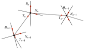
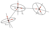
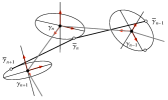
Figure 1: Deformation of a curve. Left: a discrete curve and its Frenet frame, middle: step (1) and (2), right: step(3)

The condition that $\sin(w_{n+1}+\kappa_{n+1}-w_{n-1})$ is a constant for all $n$ is equivalent to that $\overline{B}_{n}$ lies on the same side with respect to the plane spanned by $\overline{\gamma}_{n}-\gamma_{n}$ and $B_{n}$ for all $n$ (see Fig.2), and this is the necessary and sufficient condition that the deformation is torsion-preserving. We will discuss this point in Section 7.1.2.

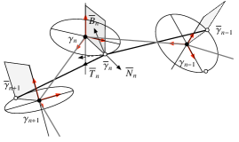
Figure 2: The necessary and sufficient condition for the preservation of the torsion. $\overline{B}$ should lie on the same side with respect to the plane spanned by $\overline{\gamma}-\gamma$ and $B$ (gray planes).

Repeating the construction in Proposition 6.1 yields the sequence of the discrete space curves with constant torsion $\gamma^{0}=\gamma,\,\gamma^{1}=\overline{\gamma},\,\gamma^{2}=\overline{\gamma^{1}},\ldots,\gamma^{m}=\overline{\gamma^{m-1}},\ldots$. Correspondingly, we write the data $\kappa$, $T$, $N$, $B$ associated with the discrete curve as $\kappa^{m}$, $T^{m}$, $N^{m}$, $B^{m}$, respectively. We also write the data of deformation $\delta$, $b$, $\mu$ as $\delta_{m}$, $b_{m}$, $\mu_{m}$, respectively. The following theorem is derived immediately by applying Proposition 6.1 successively.

Theorem 6.2.

Let $\gamma^{0}$ be a discrete space curve with the constant torsion $\lambda$. We define the sequence of discrete space curves $\gamma^{m}$ by

$$\gamma^{m+1}_{n}=\gamma^{m}_{n}+\delta_{m}\left(\cos w^{m}_{n}T^{m}_{n}+\sin w^{m}_{n}N^{m}_{n}\right),$$ (6.9)

$$\delta_{m}=\dfrac{b_{m}}{1+\frac{b_{m}^{2}\lambda^{2}}{4}}>0\,,$$ (6.10)

$$w^{m}_{n+1}=-\kappa^{m}_{n+1}+2\arctan\dfrac{b_{m}+a_{n}}{b_{m}-a_{n}}\tan\dfrac{w^{m}_{n}}{2},$$ (6.11)

where $a_{n}$ is determined from the data $\epsilon$, $\nu$ of the initial curve $\gamma^{0}$ by (4.15). We require that the sequences $b_{m}>0$ and $w_{0}^{m}$ should be chosen so that the sign of $\sin(w_{n+1}^{m}+\kappa_{n+1}^{m}-w_{n-1}^{m})$ is constant for all $n$. Then we have the following:

1. (Isoperimetricity and preservation of the torsion) For all $m$, $\gamma^{m}$ satisfies

   $$\left|\gamma^{m}_{n+1}-\gamma^{m}_{n}\right|=\epsilon_{n},$$ (6.12)

   and the torsion of $\gamma^{m}$ is $\lambda$. Namely, (6.9) gives a isoperimetric and torsion-preserving deformation.

2. (Deformation of the Frenet frame) The Frenet frame $\varPhi^{m}_{n}=\left[T^{m}_{n},N^{m}_{n},B^{m}_{n}\right]$ satisfies

   $$\varPhi^{m}_{n+1}=\varPhi^{m}_{n}L^{m}_{n},\quad\varPhi^{m+1}_{n}=\varPhi^{m}_{n}M^{m}_{n}.$$ (6.13)

   Here,

   $$L^{m}_{n}=R_{1}\left(-\nu_{n+1}\right)R_{3}\left(\kappa^{m}_{n+1}\right),\quad\nu_{n+1}=2\arctan\dfrac{a_{n}\lambda}{2},$$ (6.14)

   and $M_{n}^{m}$ is given by either of the following for each $m$: in case of $\sin(w_{n+1}^{m}+\kappa_{n+1}^{m}-w_{n-1}^{m})>0$,

   $$M^{m}_{n}=R_{3}\left(w^{m}_{n}\right)R_{1}\left(\mu_{m}\right)R_{3}\left(w^{m}_{n+1}+\kappa^{m}_{n+1}\right),\quad\mu_{m}=-2\arctan\dfrac{b_{m}\lambda}{2},$$ (6.15)

   or in case of $\sin(w_{n+1}^{m}+\kappa_{n+1}^{m}-w_{n-1}^{m})<0$,

   $$M^{m}_{n}=R_{3}\left(w^{m}_{n}\right)R_{1}\left(\mu_{m}\right)R_{3}\left(-w^{m}_{n+1}-\kappa^{m}_{n+1}\right),\quad\mu_{m}=2\arctan\dfrac{2}{b_{m}\lambda}.$$ (6.16)

   Choosing the matrix $M$ as (6.15), then $L,M$ are the Lax pair of the discrete mKdV equation. Namely, the compatibility condition $L_{n}^{m}M_{n+1}^{m}=M_{n}^{m}L_{n}^{m+1}$ for the system of difference equation with respect to $\varPhi^{m}_{n}$ (6.13) gives

   $$w_{n+1}^{m}-w_{n-1}^{m}=\kappa_{n}^{m+1}-\kappa_{n+1}^{m}.$$ (6.17)

   Then (6.11) and (6.17) yield the discrete mKdV equation

   $$\dfrac{w^{m+1}_{n+1}}{2}-\dfrac{w^{m}_{n}}{2}=\arctan\left(\dfrac{b_{m+1}+a_{n}}{b_{m+1}-a_{n}}\tan\dfrac{w^{m+1}_{n}}{2}\right)-\arctan\left(\dfrac{b_{m}+a_{n+1}}{b_{m}-a_{n+1}}\tan\dfrac{w^{m}_{n+1}}{2}\right).$$ (6.18)

   Choosing the matrix $M$ as (6.16), then $L,M$ are the Lax pair of the discrete sine-Gordon equation. Namely, the compatibility condition of (6.13) gives

   $$w_{n+1}^{m}-w_{n-1}^{m}=-\kappa_{n}^{m+1}-\kappa_{n+1}^{m},$$ (6.19)

   and then (6.11) and (6.19) yields the discrete sine-Gordon equation

   $$\dfrac{w^{m+1}_{n+1}}{2}+\dfrac{w^{m}_{n}}{2}=\arctan\left(\dfrac{b_{m+1}+a_{n}}{b_{m+1}-a_{n}}\tan\dfrac{w^{m+1}_{n}}{2}\right)+\arctan\left(\dfrac{b_{m}+a_{n+1}}{b_{m}-a_{n+1}}\tan\dfrac{w^{m}_{n+1}}{2}\right).$$ (6.20)

Remark 6.3.

1. The deformation of the form (6.9), (6.10) has been obtained in [5] as the Bäcklund transformation of the space smooth curve with constant torsion.

2. The discrete sine-Gordon equation (6.20) can be rewritten as the well-known form[12]

   $$\sin\frac{\theta_{n+1}^{m+1}-\theta_{n}^{m+1}-\theta_{n+1}^{m}+\theta_{n}^{m}}{4}=\frac{a_{n}}{b_{m}}\sin\frac{\theta_{n+1}^{m+1}+\theta_{n}^{m+1}+\theta_{n+1}^{m}+\theta_{n}^{m}}{4}$$ (6.21)

   by the dependent variable transformation

   $$w_{n}^{m}=-\frac{\theta_{n}^{m+1}+\theta_{n+1}^{m}}{2}.$$ (6.22)

It is also possible for this case to reconstruct the discrete curves from the Frenet frame by using the Sym-Tafel formula. Lifting the Frenet frame $\varPhi=[T,N,B]\in\mathrm{SO}(3)$ to the $\mathrm{SU}(2)$-valued function $\phi$ by using Proposition 2.2, then $\phi$ satisfies

$$\phi_{n+1}^{m}=\phi_{n}^{m}L_{n}^{m},\quad L_{n}^{m}=\pm\left[\begin{array}[]{cc}e^{-\frac{\sqrt{-1}}{2}\nu_{n+1}}&0\\ 0&e^{\frac{\sqrt{-1}}{2}\nu_{n+1}}\end{array}\right]R\left(\frac{\kappa_{n+1}^{m}}{2}\right),\quad\nu_{n+1}=2\arctan\frac{a_{n}\lambda}{2},$$ (6.25)

and

$$\begin{split}\phi_{n}^{m+1}=\phi_{n}^{m}M_{n}^{m},\quad&M_{n}^{m}=\pm R\left(\frac{w_{n}^{m}}{2}\right)\left[\begin{array}[]{cc}e^{\frac{\sqrt{-1}}{2}\mu_{m}}&0\\ 0&e^{-\frac{\sqrt{-1}}{2}\mu_{m}}\end{array}\right]R\left(\frac{w_{n+1}^{m}+\kappa_{n+1}^{m}}{2}\right),\\ &\mu_{m}=-2\arctan\frac{b_{m}\lambda}{2},\end{split}$$ (6.26)

or

$$\begin{split}\phi_{n}^{m+1}=\phi_{n}^{m}M_{n}^{m},\quad&M_{n}^{m}=\pm R\left(\frac{w_{n}^{m}}{2}\right)\left[\begin{array}[]{cc}e^{\frac{\sqrt{-1}}{2}\mu_{m}}&0\\ 0&e^{-\frac{\sqrt{-1}}{2}\mu_{m}}\end{array}\right]R\left(-\frac{w_{n+1}^{m}+\kappa_{n+1}^{m}}{2}\right),\\ &\mu_{m}=2\arctan\frac{2}{b_{m}\lambda},\end{split}$$ (6.27)

where

$$R(\theta)=\left[\begin{array}[]{cc}\cos\theta&-\sin\theta\\ \sin\theta&\cos\theta\end{array}\right].$$ (6.28)

Theorem 6.4.

For a constant $\lambda$ and sequences $a_{n}$, $b_{m}$, $w_{n}^{0}$, $w_{0}^{m}$, we define the functions $w$ and $\kappa$ by (6.18) and (6.11) respectively, and let $\phi$ be a solution to the system of difference equations (6.25), (6.26). Then let $f$ be the isomorphism defined by (2.3) and put

$$\gamma^{m}_{n}=f^{-1}\left(S^{m}_{n}\right),\quad S^{m}_{n}=-\left(\dfrac{\partial}{\partial\lambda}\phi^{m}_{n}\right)\left(\phi^{m}_{n}\right)^{-1}.$$ (6.29)

Then, for each $m$, $\gamma$ is a discrete space curve with the following properties: (1) the distances between the contiguous vertices are given by

$$\left|\gamma_{n+1}^{m}-\gamma_{n}^{m}\right|=\epsilon_{n}=\dfrac{a_{n}}{1+\frac{a_{n}^{2}\lambda^{2}}{4}},\quad\left|\gamma_{n}^{m+1}-\gamma_{n}^{m}\right|=\delta_{m}=\dfrac{b_{m}}{1+\frac{b_{m}^{2}\lambda^{2}}{4}},$$ (6.30)

(2) the angles between the contiguous tangent vectors are $\kappa_{n}^{m}$, (3) the angles between the contiguous binormal vectors are $\nu_{n}^{m}$, (4) the angles between $\gamma_{n}^{m+1}-\gamma_{n}^{m}$ and $\gamma_{n+1}^{m}-\gamma_{n}^{m}$ are $w_{n}^{m}$. Namely, $\gamma$ is a torsion-preserving isoperimetric and equidistant deformation of the discrete space curves with constant torsion described by the discrete mKdV equation. Similarly, if we determine the function $w$ and $\kappa$ by (6.20) and (6.11) respectively, and let $\phi$ be a solution to the system of difference equations (6.25), (6.27), then (6.29) gives a torsion-preserving isoperimetric and equidistant deformation of the discrete space curves with constant torsion described by the discrete sine-Gordon equation.

In Theorem 6.2 (2), it is the necessary and sufficient condition for the deformation of the discrete curve $\gamma^{m}\mapsto\gamma^{m+1}$ being torsion-preserving that the sign of $\sin(w_{n+1}^{m}+\kappa_{n+1}^{m}-w_{n-1}^{m})$ is constant as a function of $n$ at each $m$. On the other hand, given an initial curve $\gamma_{n}^{0}$ (accordingly $a_{n}$, $\kappa_{n}^{0}$ and $\lambda$), the deformation of the curve is uniquely determined if we specify $w_{0}^{m}$ and $b_{m}$. Therefore, the necessary and sufficient condition for the preservation of the torsion may be described as the condition of $w_{0}^{m}$ and $b_{m}$ for given $a_{n}$, $\kappa_{n}^{0}$ and $\lambda$. However, it is practically difficult to write down this condition. Instead, we can show the following proposition as a sufficient condition.

Proposition 6.5.

1. In the discrete deformation of the discrete curves in Theorem 6.2, if we choose $b_{m}>0$ to satisfy either of the following conditions at each $m$, then the deformation is torsion-preserving.

   $$\begin{split}\mbox{(i)}&\quad b_{m}>\max\left\{\frac{a_{\rm max}}{\tan\frac{\kappa_{\rm min}^{m}}{4}},\frac{\Delta a}{2\cos\frac{\kappa_{\max}^{m}}{2}}\left(1+\sqrt{1+\frac{4a_{\min}a_{\max}}{(\Delta a)^{2}}\cos^{2}\frac{\kappa_{\rm max}^{m}}{2}}\right)\right\}\\ &\quad\mbox{or}\\ \mbox{(ii)}&\quad b_{m}<\min\left\{a_{\rm min}\tan\frac{\kappa_{\rm min}^{m}}{4},\frac{\Delta a}{2\cos\frac{\kappa_{\max}^{m}}{2}}\left(-1+\sqrt{1+\frac{4a_{\min}a_{\max}}{(\Delta a)^{2}}\cos^{2}\frac{\kappa_{\rm max}^{m}}{2}}\right)\right\},\end{split}$$ (6.31)

   where

   $$\kappa_{\mathrm{min}}^{m}=\min_{n}\kappa_{n}^{m},\ \kappa_{\mathrm{max}}^{m}=\max_{n}\kappa_{n}^{m},\ a_{\rm max}=\max_{n}a_{n},\quad a_{\rm min}=\min_{n}a_{n},\ \Delta a=a_{\rm max}-a_{\rm min}.$$ (6.32)

2. In the case of (i), the Frenet frame $\Phi$ is deformed according to (6.13), (6.14), (6.16), and in the case of (ii) it is deformed according to (6.13), (6.14), (6.15). Namely, (i) and (ii) correspond to the deformation by the discrete sine-Gordon equation (6.20) and discrete mKdV equation (6.18) respectively.

7 Proof of Main Results

7.1 Proof of Proposition 6.1

7.1.1 Isoperimetricity

We show that $|\overline{\gamma}_{n+1}-\overline{\gamma}_{n}|=\epsilon_{n}$ holds if we give the deformation of the curves by (6.2) and $|\gamma_{n+1}-\gamma_{n}|=\epsilon_{n}$. Since we have from direct computation that

$$|\overline{\gamma}_{n+1}-\overline{\gamma}_{n}|^{2} =\epsilon_{n}^{2}+2\delta^{2}\left[1-\cos(w_{n+1}+\kappa_{n+1})\cos w_{n}-\cos\nu_{n+1}\sin(w_{n+1}+\kappa_{n+1})\sin w_{n}\right]$$

$$+2\epsilon_{n}\delta\left[\cos(w_{n+1}+\kappa_{n+1})-\cos w_{n}\right],$$

it suffices to show

$$\begin{split}\delta&\left[1-\cos(w_{n+1}+\kappa_{n+1})\cos w_{n}-\cos\nu_{n+1}\sin(w_{n+1}+\kappa_{n+1})\sin w_{n}\right]\\ &+\epsilon_{n}\left[\cos(w_{n+1}+\kappa_{n+1})-\cos w_{n}\right]=0.\end{split}$$

Noticing that

$$\epsilon_{n}=\frac{a_{n}}{1+\frac{a_{n}^{2}\lambda^{2}}{4}},\quad\delta=\frac{b}{1+\frac{b^{2}\lambda^{2}}{4}},\quad\lambda=\frac{2}{a_{n}}\tan\frac{\nu_{n+1}}{2},$$

the above equation can be rewritten as

$$\begin{split}&\left(\frac{\lambda^{2}a_{n}b}{4}\sin\frac{w_{n+1}+\kappa_{n+1}+w_{n}}{2}-\sin\frac{w_{n+1}+\kappa_{n+1}-w_{n}}{2}\right)\\ &\times\left(a_{n}\sin\frac{w_{n+1}+\kappa_{n+1}+w_{n}}{2}-b\sin\frac{w_{n+1}+\kappa_{n+1}-w_{n}}{2}\right)=0,\end{split}$$ (7.1)

which holds since the second factor becomes $0$ by (6.4).

Remark 7.1.

The deformation such that the first factor of (7.1) becomes $0$ is also consistent with (6.2) and (6.3). See Remark 7.3 in the end of this section.

7.1.2 Preservation of the Torsion

We next show that $\nu$ is invariant by the deformation. Since $\nu_{n+1}\in[-\pi,\pi)$, we have to show that $\cos\overline{\nu}_{n+1}=\cos\nu_{n+1}$ and $\sin\overline{\nu}_{n+1}=\sin\nu_{n+1}$. Noticing that $\cos\nu_{n+1}=\langle B_{n},B_{n+1}\rangle$ and $\sin\nu_{n+1}=\langle N_{n},B_{n+1}\rangle$, we start from the computation of $\overline{T}_{n}$. From (6.2), we introduce the displacement vector $D_{n}$ by

$$D_{n}=\frac{\overline{\gamma}_{n}-\gamma_{n}}{\delta}=\varPhi_{n}\left[\begin{array}[]{c}\cos w_{n}\\ \sin w_{n}\\ 0\end{array}\right],$$ (7.2)

then it follows by definition that

$$\delta\,D_{n}+\epsilon_{n}\,\overline{T}_{n}=\epsilon_{n}\,T_{n}+\delta\,D_{n+1}.$$ (7.3)

We have by noticing $\lambda=\frac{2}{a_{n}}\tan\frac{\nu_{n+1}}{2}$

$$\overline{T}_{n}=\frac{\delta}{\epsilon_{n}}D_{n+1}-\frac{\delta}{\epsilon_{n}}D_{n}+T_{n}=\frac{\delta}{\epsilon_{n}}\varPhi_{n+1}\left[\begin{array}[]{c}\cos w_{n+1}\\ \sin w_{n+1}\\ 0\end{array}\right]-\frac{\delta}{\epsilon_{n}}\varPhi_{n}\left[\begin{array}[]{c}\cos w_{n}\\ \sin w_{n}\\ 0\end{array}\right]+\varPhi_{n}\left[\begin{array}[]{c}1\\ 0\\ 0\end{array}\right]$$ (7.13)

$$=\varPhi_{n}^{m}\left\{\frac{\delta}{\epsilon_{n}}\left(L_{n}\left[\begin{array}[]{c}\cos w_{n+1}\\ \sin w_{n+1}\\ 0\end{array}\right]-\left[\begin{array}[]{c}\cos w_{n}\\ \sin w_{n}\\ 0\end{array}\right]\right)+\left[\begin{array}[]{c}1\\ 0\\ 0\end{array}\right]\right\}$$ (7.23)

$$=\frac{1}{1+\frac{b^{2}\lambda^{2}}{4}}\varPhi_{n}\left[\begin{array}[]{c}\vskip 6.0pt plus 2.0pt minus 2.0pt\cos 2U_{n}+\dfrac{b^{2}\lambda^{2}}{4}\cos 2V_{n}\\ \vskip 6.0pt plus 2.0pt minus 2.0pt\sin 2U_{n}-\dfrac{b^{2}\lambda^{2}}{4}\sin 2V_{n}\\ -b\lambda\sin(U_{n}+V_{n})\end{array}\right].$$ (7.27)

Here, we put

$$U_{n}=\frac{w_{n+1}+\kappa_{n+1}+w_{n}}{2},\quad V_{n}=\frac{w_{n+1}+\kappa_{n+1}-w_{n}}{2}$$ (7.28)

and used

$$a_{n}\sin U_{n}=b\sin V_{n},$$ (7.29)

which follows from (6.4). Moreover, from

$$\overline{T}_{n-1} =\frac{1}{1+\frac{b^{2}\lambda^{2}}{4}}\varPhi_{n-1}\left[\begin{array}[]{c}\vskip 6.0pt plus 2.0pt minus 2.0pt\cos 2U_{n-1}+\dfrac{b^{2}\lambda^{2}}{4}\cos 2V_{n-1}\\ \vskip 6.0pt plus 2.0pt minus 2.0pt\sin 2U_{n-1}-\dfrac{b^{2}\lambda^{2}}{4}\sin 2V_{n-1}\\ -b\lambda\sin(U_{n-1}+V_{n-1})\end{array}\right]$$

$$=\frac{1}{1+\frac{b^{2}\lambda^{2}}{4}}\varPhi_{n}\left(L_{n-1}\right)^{-1}\left[\begin{array}[]{c}\vskip 6.0pt plus 2.0pt minus 2.0pt\cos 2U_{n-1}+\dfrac{b^{2}\lambda^{2}}{4}\cos 2V_{n-1}\\ \vskip 6.0pt plus 2.0pt minus 2.0pt\sin 2U_{n-1}-\dfrac{b^{2}\lambda^{2}}{4}\sin 2V_{n-1}\\ -b\lambda\sin(U_{n-1}+V_{n-1})\end{array}\right],$$

a tedious but straightforward calculation by using (6.4) yields

$$\overline{T}_{n-1}\times\overline{T}_{n} =\frac{\sin(w_{n+1}+\kappa_{n+1}-w_{n-1})}{1+\frac{b^{2}\lambda^{2}}{4}}\varPhi_{n}\left[\begin{array}[]{c}-b\lambda\sin w_{n}\\ b\lambda\cos w_{n}\\ 1-\frac{b^{2}\lambda^{2}}{4}\end{array}\right],$$ (7.33)

from which we obtain

$$\overline{B}_{n}=\frac{\overline{T}_{n-1}\times\overline{T}_{n}}{\left|\overline{T}_{n-1}\times\overline{T}_{n}\right|}=\frac{\operatorname{sgn}(\sin(w_{n+1}+\kappa_{n+1}-w_{n-1}))}{1+\frac{b^{2}\lambda^{2}}{4}}\varPhi_{n}\left[\begin{array}[]{c}-b\lambda\sin w_{n}\\ b\lambda\cos w_{n}\\ 1-\frac{b^{2}\lambda^{2}}{4}\end{array}\right],$$ (7.34)

$$\overline{B}_{n+1} =\frac{\operatorname{sgn}(\sin(w_{n+2}+\kappa_{n+2}-w_{n}))}{1+\frac{b^{2}\lambda^{2}}{4}}\varPhi_{n}L_{n}\left[\begin{array}[]{c}-b\lambda\sin w_{n+1}\\ b\lambda\cos w_{n+1}\\ 1-\frac{b^{2}\lambda^{2}}{4}\end{array}\right]$$ (7.38)

$$=\frac{\operatorname{sgn}(\sin(w_{n+2}+\kappa_{n+2}-w_{n}))}{1+\frac{b^{2}\lambda^{2}}{4}}\varPhi_{n}\left[\begin{array}[]{c}\vskip 6.0pt plus 2.0pt minus 2.0pt-b\lambda\sin(\kappa_{n+1}+w_{n+1})\\ \vskip 6.0pt plus 2.0pt minus 2.0pt\frac{\lambda\left\{b(1-\frac{a_{n}^{2}\lambda^{2}}{4})\cos(\kappa_{n+1}+w_{n+1})+a_{n}(1-\frac{b^{2}\lambda^{2}}{4})\right\}}{1+\frac{a_{n}^{2}\lambda^{2}}{4}}\\ -\frac{a_{n}b\lambda^{2}\cos(\kappa_{n+1}+w_{n+1})-(1-\frac{a_{n}^{2}\lambda^{2}}{4})(1-\frac{b^{2}\lambda^{2}}{4})}{1+\frac{a_{n}^{2}\lambda^{2}}{4}}\end{array}\right].$$ (7.42)

Moreover, from $\overline{N}_{n}=\overline{B}_{n}\times\overline{T}_{n}$ we have

$$\overline{N}_{n}=\frac{\operatorname{sgn}(\sin(w_{n+1}+\kappa_{n+1}-w_{n-1}))}{1+\frac{b^{2}\lambda^{2}}{4}}\varPhi_{n}\left[\begin{array}[]{c}\vskip 6.0pt plus 2.0pt minus 2.0pt-\sin 2U_{n}-\dfrac{b^{2}\lambda^{2}}{4}\sin 2V_{n}\\ \vskip 6.0pt plus 2.0pt minus 2.0pt\cos 2U_{n}-\dfrac{b^{2}\lambda^{2}}{4}\cos 2V_{n}\\ -b\lambda\cos(U_{n}+V_{n})\end{array}\right].$$ (7.43)

Therefore, if $\operatorname{sgn}(\sin(w_{n+2}+\kappa_{n+2}-w_{n}))=\operatorname{sgn}(\sin(w_{n+1}+\kappa_{n+1}-w_{n-1}))$ holds, then we have by using (6.4) that

$$\cos\overline{\nu}_{n+1}=\langle\overline{B}_{n},\overline{B}_{n+1}\rangle=\frac{1-\frac{a_{n}^{2}\lambda^{2}}{4}}{1+\frac{a_{n}^{2}\lambda^{2}}{4}}=\frac{1-\tan^{2}\frac{\nu_{n+1}}{2}}{1+\tan^{2}\frac{\nu_{n+1}}{2}}=\cos\nu_{n+1},$$ (7.44)

$$\sin\overline{\nu}_{n+1}=\langle\overline{B}_{n+1},\overline{N}_{n}\rangle=\frac{a_{n}\lambda}{1+\frac{a_{n}^{2}\lambda^{2}}{4}}=\frac{2\tan\frac{\nu_{n+1}}{2}}{1+\tan^{2}\frac{\nu_{n+1}}{2}}=\sin\nu_{n+1},$$ (7.45)

which implies $\overline{\nu}_{n+1}=\nu_{n+1}$. ∎

Remark 7.2.

The above discussion shows that the condition that $\operatorname{sgn}(\sin(w_{n+1}+\kappa_{n+1}-w_{n-1}))$ is constant with respect to $n$ is the necessary and sufficient condition for the deformation being torsion-preserving. Since we see from (7.2) and (7.34) that $\operatorname{sgn}(\sin(w_{n+1}+\kappa_{n+1}-w_{n-1}))=\operatorname{sgn}(\langle D_{n}\times B_{n},\overline{B}_{n}\rangle)$, the geometric meaning of this condition is that $\overline{B}_{n}$ lie on the same side with respect to the plane spanned by $D_{n}$ and $B_{n}$ for all $n$.

7.1.3 Deformation of the Frenet Frame

For $\varPhi_{n}=[T_{n},N_{n},B_{n}]\in{\rm SO}(3)$, we construct $M_{n}\in{\rm SO}(3)$ satisfying

$$\varPhi_{n+1}=\varPhi_{n}L_{n},\quad\overline{\varPhi}_{n}=\varPhi_{n}M_{n}.$$ (7.46)

In the calculations in the previous section, since the column vectors of $M_{n}$ are given by the right-hand side of (7.27), (7.43) and (7.34), respectively, we have for $\sin(w_{n+1}+\kappa_{n+1}-w_{n-1})>0$

$$M_{n} =\frac{1}{1+\frac{b^{2}\lambda^{2}}{4}}\small\left[\begin{array}[]{ccc}\cos 2U_{n}+\dfrac{b^{2}\lambda^{2}}{4}\cos 2V_{n}&-\sin 2U_{n}-\dfrac{b^{2}\lambda^{2}}{4}\sin 2V_{n}&-b\lambda\sin w_{n}\\ \sin 2U_{n}-\dfrac{b^{2}\lambda^{2}}{4}\sin 2V_{n}&\cos 2U_{n}-\dfrac{b^{2}\lambda^{2}}{4}\cos 2V_{n}&b\lambda\cos w_{n}\\ -b\lambda\sin(U_{n}+V_{n})&-b\lambda\cos(U_{n}+V_{n})&1-\frac{b^{2}\lambda^{2}}{4}\end{array}\right]$$ (7.50)

$$=R_{3}(w_{n})R_{1}(\mu)R_{3}(w_{n+1}+\kappa_{n+1}),\quad\mu=-2\arctan\frac{b\lambda}{2}.$$ (7.51)

Similarly, we have for $\sin(w_{n+1}+\kappa_{n+1}-w_{n-1})<0$

$$M_{n} =\frac{1}{1+\frac{b^{2}\lambda^{2}}{4}}\small\left[\begin{array}[]{ccc}\cos 2U_{n}+\dfrac{b^{2}\lambda^{2}}{4}\cos 2V_{n}&\sin 2U_{n}+\dfrac{b^{2}\lambda^{2}}{4}\sin 2V_{n}&b\lambda\sin w_{n}\\ \sin 2U_{n}-\dfrac{b^{2}\lambda^{2}}{4}\sin 2V_{n}&-\cos 2U_{n}+\dfrac{b^{2}\lambda^{2}}{4}\cos 2V_{n}&-b\lambda\cos w_{n}\\ -b\lambda\sin(U_{n}+V_{n})&b\lambda\cos(U_{n}+V_{n})&-1+\frac{b^{2}\lambda^{2}}{4}\end{array}\right]$$ (7.55)

$$=R_{3}(w_{n})R_{1}(\mu)R_{3}(-w_{n+1}-\kappa_{n+1}),\quad\mu=2\arctan\frac{2}{b\lambda}.$$ (7.56)

∎

7.2 Proof of Theorem 6.4

If the Frenet frame $\varPhi=\left[T,N,B\right]\in\mathrm{SO}(3)$ satisfies (6.13), (6.14) and (6.15), the corresponding $\mathrm{SU}(2)$-valued function $\phi$ satisfy (6.25) and (6.26). In particular, (6.26) is rewritten as

$$\phi_{n}^{m+1}=\phi_{n}^{m}M_{n}^{m},\ M_{n}^{m}=\dfrac{\pm 1}{\sqrt{1+\frac{b_{m}^{2}\lambda^{2}}{4}}}\left[\begin{array}[]{cc}\vskip 6.0pt plus 2.0pt minus 2.0pt\cos U_{n}^{m}-\frac{\sqrt{-1}b_{m}\lambda}{2}\cos V_{n}^{m}&-\sin U_{n}^{m}+\frac{\sqrt{-1}b_{m}\lambda}{2}\sin V_{n}^{m}\\ \sin U_{n}^{m}+\frac{\sqrt{-1}b_{m}\lambda}{2}\sin V_{n}^{m}&\cos U_{n}^{m}+\frac{\sqrt{-1}b_{m}\lambda}{2}\cos V_{n}^{m}\end{array}\right],$$ (7.57)

where $U_{n}^{m}$ and $V_{n}^{m}$ are given by (7.28). Putting

$$T^{m}_{n}=\phi_{n}^{m}e_{1}\left(\phi_{n}^{m}\right)^{-1},\quad N_{n}^{m}=\phi_{n}^{m}e_{2}\left(\phi_{n}^{m}\right)^{-1},\quad B_{n}^{m}=\phi_{n}^{m}e_{3}\left(\phi_{n}^{m}\right)^{-1},$$ (7.58)

$S_{n}^{m}=-(\phi_{n}^{m})_{\lambda}(\phi_{n}^{m})^{-1}$ satisfies

$$S_{n}^{m+1}-S_{n}^{m} =-\phi_{n}^{m}(M_{n}^{m})_{\lambda}(M_{n}^{m})^{-1}(\phi_{n}^{m})^{-1}=-\phi_{n}^{m}\left\{\frac{-b_{m}}{1+\frac{b_{m}^{2}\lambda^{2}}{4}}(\cos w_{n}^{m}e_{1}+\sin w_{n}^{m}e_{2})\right\}(\phi_{n}^{m})^{-1}$$

$$=\delta_{m}\left(\cos w_{n}^{m}T_{n}^{m}+\sin w_{n}^{m}N_{n}^{m}\right),$$ (7.59)

which coincides with the definition of the deformation (6.9). Similarly, if $\varPhi$ satisfies (6.13), (6.14) and (6.16), then it follows that $\phi$ satisfies (6.25) and (6.27). Then (7.59) is derived in a similar manner. ∎

Remark 7.3.

The deformation satisfying the condition

$$\frac{\lambda^{2}a_{n}b}{4}\sin\frac{w_{n+1}+\kappa_{n+1}+w_{n}}{2}-\sin\frac{w_{n+1}+\kappa_{n+1}-w_{n}}{2}=0$$ (7.60)

or

$$w_{n+1}=-\kappa_{n+1}+2\arctan\dfrac{\hat{b}+a_{n}}{\hat{b}-a_{n}}\tan\dfrac{w_{n}}{2},\quad\hat{b}=\frac{4}{b\lambda^{2}}$$ (7.61)

which eliminates the first factor of (7.1) is consistent with (6.2) and (6.3). This deformation is obtained from the invariance of $\delta$ with respect to the transformation $b\mapsto\hat{b}$. We do not discuss this deformation further since all of the above results can be rewritten as those of this deformation by the redefinition of the parameter $b\mapsto\hat{b}$.

7.3 Proof of Proposition 6.5

We fix $m$. Noticing (6.11), $\sin(w_{n+1}^{m}+\kappa_{n+1}^{m}-w_{n-1}^{m})$ can be rewritten as

For simplicity, we put

$$\tan\frac{w_{n}^{m}}{2}=W,\quad\tan\frac{\kappa_{n}^{m}}{2}=K,\quad\quad c=\frac{b_{m}-a_{n}}{b_{m}+a_{n}},\quad\underline{c}=\frac{b_{m}-a_{n-1}}{b_{m}+a_{n-1}}.$$ (7.63)

Here since we have $a_{n},b_{m}>0$, $\kappa_{n}^{m}\in(0,\pi)$ and $w_{n}^{m}\in[-\pi,\pi)$, it follows that

$$-1<c<1,\quad-1<\underline{c}<1,\quad K>0,\quad-\infty<W<\infty.$$ (7.64)

Noticing

$$\sin(2\arctan x-2\arctan y)=\frac{2(1+xy)(x-y)}{(1+x^{2})(1+y^{2})},$$

(7.62) can be rewritten as

$$\sin(w_{n+1}^{m}+\kappa_{n+1}^{m}-w_{n-1}^{m})=\frac{-\left\{\underline{c}W^{2}+K(\underline{c}-c)W+c\right\}\left\{KW^{2}+(c\underline{c}-1)W+Kc\underline{c}\right\}}{(1+\frac{W^{2}}{c^{2}})\left[1+\left(\underline{c}\frac{W+K}{1-WK}\right)^{2}\right](1-KW)^{2}c^{2}}.$$ (7.65)

Now we require that for arbitrary $W$ the sign of (7.65) is constant for all $n$. To this end, since the denominator of the right-hand side does not affect the sign, it is sufficient that discriminants of the two factors of the numerator which are quadratic in $W$ are negative. Therefore, we determine $b_{m}$ such that both of the inequalities

$$\begin{split}&K^{2}(c-\underline{c})^{2}-4c\underline{c}<0,\\ &(c\underline{c}-1)^{2}-4K^{2}c\underline{c}<0\end{split}$$ (7.66)

are satisfied simultaneously. Solving the inequalities (7.66), we have

$$\left(\sqrt{K^{2}+1}-K\right)^{2}<c\underline{c}<\left(\sqrt{K^{2}+1}+K\right)^{2},$$ (7.67)

$$\left(\frac{\sqrt{K^{2}+1}-1}{K}\right)^{2}<\frac{c}{\underline{c}}<\left(\frac{\sqrt{K^{2}+1}+1}{K}\right)^{2}.$$ (7.68)

(7.67) and (7.68) imply that the contiguous $c_{n}$ with respect to $n$ must have the same sign, namely, for each $m$, $c_{n}$ must have the same sign for all $n$. So we put

$$a_{\rm max}=\max_{n}a_{n},\ a_{\rm min}=\min_{n}a_{n},\ c_{\rm max}=\max_{n}c_{n}=\frac{b_{m}-a_{\rm min}}{b_{m}+a_{\rm min}},\ c_{\rm min}=\min_{n}c_{n}=\frac{b_{m}-a_{\rm max}}{b_{m}+a_{\rm max}},$$ (7.69)

and we divide the discussion into two cases; (i) $c_{\rm min},c_{\rm max}>0$ ($b_{m}>a_{\rm max}$) and (ii) $c_{\rm min},c_{\max}<0$ ($b_{m}<a_{\rm min}$).

(i) The case of $c_{\rm min},c_{\rm max}>0$ ($b_{m}>a_{\rm max}$). From (7.67), (7.68), it is sufficient to find the condition such that the following inequalities

$$\left(\sqrt{K^{2}+1}-K\right)^{2}<c_{\rm min}^{2}\leq c_{\rm max}^{2}<\left(\sqrt{K^{2}+1}+K\right)^{2},$$ (7.70)

$$\left(\frac{\sqrt{K^{2}+1}-1}{K}\right)^{2}<\frac{c_{\rm min}}{c_{\rm max}}\leq\frac{c_{\rm max}}{c_{\rm min}}<\left(\frac{\sqrt{K^{2}+1}+1}{K}\right)^{2}$$ (7.71)

are satisfied simultaneously. Solving (7.70) and (7.71) in terms of $b_{m}$ by noticing (7.64), (7.69) and

$$\frac{\sqrt{K^{2}+1}-1}{K}=\tan\frac{\kappa_{n}^{m}}{4},\quad\frac{\sqrt{K^{2}+1}+1}{K}=\frac{1}{\tan\frac{\kappa_{n}^{m}}{4}},$$ (7.72)

we have

$$b_{m}>\frac{a_{\rm max}}{\tan\frac{\kappa_{n}^{m}}{4}},\quad b_{m}>\frac{\Delta a}{2\cos^{2}\frac{\kappa_{n}^{m}}{2}}\left(1+\sqrt{1+\frac{4a_{\rm min}a_{\max}}{(\Delta a)^{2}}\cos^{2}\frac{\kappa_{n}^{m}}{2}}\right),$$ (7.73)

respectively. Note that the right-hand sides of the first and the second inequalities are monotonic decreasing and monotonic increasing with respect to $\kappa_{n}^{m}$ respectively. Therefore it is sufficient to choose $b_{m}$ as

$$b_{m}>\max\left\{\frac{a_{\rm max}}{\tan\frac{\kappa_{\rm min}^{m}}{4}},\frac{\Delta a}{2\cos\frac{\kappa_{\rm max}^{m}}{2}}\left(1+\sqrt{1+\frac{4a_{\rm min}a_{\max}}{(\Delta a)^{2}}\cos^{2}\frac{\kappa_{\rm max}^{m}}{2}}\right)\right\},$$ (7.74)

in order for those inequalities to hold for all $n$.

(ii) The case of $c_{\rm min},c_{\rm max}<0$ ($b_{m}<a_{\rm max}$). From (7.67), (7.68) we have the following inequalities:

$$\left(\sqrt{K^{2}+1}-K\right)^{2}<c_{\rm max}^{2}\leq c_{\rm min}^{2}<\left(\sqrt{K^{2}+1}+K\right)^{2},$$ (7.75)

$$\left(\frac{\sqrt{K^{2}+1}-1}{K}\right)^{2}<\frac{c_{\rm max}}{c_{\rm min}}\leq\frac{c_{\rm min}}{c_{\rm max}}<\left(\frac{\sqrt{K^{2}+1}+1}{K}\right)^{2}.$$ (7.76)

Solving these inequalities in a similar manner to the case of (i), we find that it is sufficient to choose $b_{m}$ as

$$b_{m}<\min\left\{a_{\rm min}\tan\frac{\kappa_{\rm min}^{m}}{4},\frac{\Delta a}{2\cos^{2}\frac{\kappa_{\rm max}^{m}}{2}}\left(-1+\sqrt{1+\frac{4a_{\rm min}a_{\max}}{(\Delta a)^{2}}\cos^{2}\frac{\kappa_{\rm max}^{m}}{2}}\right)\right\}.$$ (7.77)

This proves (1). As to (2), noticing that $K>0$ in the right hand side of (7.65), the case of $c_{n}>0$ (namely the case of (i)) corresponds to $\sin(w^{m}_{n+1}+\kappa_{n+1}^{m}-w_{n+1}^{m})<0$, and the case of $c_{n}<0$ (namely the case of (ii)) corresponds to $\sin(w^{m}_{n+1}+\kappa_{n+1}^{m}-w_{n+1}^{m})>0$ respectively. Moreover, according to Section 7.1.3, we see that the former and the latter cases correspond to the deformation described by the discrete sine-Gordon equation and that described by the discrete mKdV equation respectively. ∎

8 Relation to Discrete $K$-Surfaces

The sequences of deformed discrete curves described in Theorem 6.2 form discrete surfaces in $\mathbb{R}^{3}$. We show that it is nothing but the discrete $K$-surfaces.

Definition 8.1.

If a map $\gamma:~{}\mathbb{Z}^{2}\rightarrow\mathbb{R}^{3}$, $(n,m)\mapsto\gamma_{n}^{m}$ satisfies the following conditions, we call it the discrete $K$-surface.

1. The five points $\gamma_{n}^{m}$, $\gamma_{n\pm 1}^{m}$, $\gamma_{n}^{m\pm 1}$ are coplanar. If this condition is satisfied, we say that $\gamma$ forms the discrete asymptotic net.

2. It holds that $|\gamma_{n+1}^{m}-\gamma_{n}^{m}|=|\gamma_{n+1}^{m+1}-\gamma_{n}^{m+1}|$ and $|\gamma_{n}^{m+1}-\gamma_{n}^{m}|=|\gamma_{n+1}^{m+1}-\gamma_{n+1}^{m}|$.

Proposition 8.2.

The sequence of deformed discrete curves $\gamma$ described in Theorem 6.2 form a discrete $K$-surface in $\mathbb{R}^{3}$.

Proof.

We first compute $\gamma_{n}^{m-1}$ in order to verify the condition (1) in Definition 8.1. From

$$\frac{\gamma_{n}^{m+1}-\gamma_{n}^{m}}{\delta_{m}}=\cos w_{n}^{m}T_{n}^{m}+\sin w_{n}^{m}N_{n}^{m}=\varPhi_{n}^{m}\left[\begin{array}[]{c}\cos w_{n}^{m}\\ \sin w_{n}^{m}\\ 0\end{array}\right]$$

and (6.13), we have

$$\frac{\gamma_{n}^{m}-\gamma_{n}^{m-1}}{\delta_{m-1}}=\varPhi_{n}^{m-1}\left[\begin{array}[]{c}\cos w_{n}^{m-1}\\ \sin w_{n}^{m-1}\\ 0\end{array}\right]=\varPhi_{n}^{m}(M_{n}^{m-1})^{-1}\left[\begin{array}[]{c}\cos w_{n}^{m-1}\\ \sin w_{n}^{m-1}\\ 0\end{array}\right].$$

Substituting (6.15) and (6.16) as $M_{n}^{m}$, we get

$$\gamma^{m-1}_{n}=\gamma^{m}_{n}-\delta_{m-1}\left(\cos\left(w^{m-1}_{n+1}+\kappa^{m-1}_{n+1}\right)T^{m}_{n}\mp\sin\left(w^{m-1}_{n+1}+\kappa^{m-1}_{n+1}\right)N^{m}_{n}\right),$$

Here, the cases where $M_{n}^{m}$ is given by (6.15) and (6.16) correspond to $-$ and $+$ respectively, in the right-hand side. This implies $\gamma_{n}^{m\pm 1}-\gamma_{n}^{m}\in{\rm span}\{T_{n}^{m},N_{n}^{m}\}$. Moreover, it is clear from the definition of $N_{n}^{m}$ that $\gamma_{n\pm 1}^{m}-\gamma_{n}^{m}\in{\rm span}\{T_{n}^{m},N_{n}^{m}\}$. Therefore $\gamma$ forms the discrete asymptotic net. Further, the condition (2) follows from $\left|\gamma^{m}_{n+1}-\gamma^{m}_{n}\right|=\epsilon_{n},\ \left|\gamma^{m+1}_{n}-\gamma^{m}_{n}\right|=\delta_{m}$. This proves that $\gamma$ forms a discrete $K$-surface. ∎

Remark 8.3.

Suppose that the Frenet frame $\varPhi$ satisfies (6.13), (6.14) and (6.16). Then putting

$$\varPsi^{m}_{n}=\varPhi^{m}_{n}\left[\begin{array}[]{ccc}0&0&1\\ 1&0&0\\ 0&1&0\end{array}\right]R_{1}\left(\dfrac{-\theta^{m}_{n+1}+\theta^{m}_{n}}{2}\right)$$

by using $\theta_{n}^{m}$ given in (6.22), $\varPsi$ satisfies

$$\varPsi^{m}_{n+1}=\varPsi^{m}_{n}R_{1}\left(\dfrac{\theta^{m}_{n+1}-\theta^{m}_{n}}{2}\right)R_{2}\left(-\nu_{n+1}\right)R_{1}\left(\dfrac{\theta^{m}_{n+1}-\theta^{m}_{n}}{2}\right),$$ (8.1)

$$\varPsi^{m+1}_{n}=\varPsi^{m}_{n}R_{1}\left(-\dfrac{\theta^{m+1}_{n}+\theta^{m}_{n}}{2}\right)R_{2}\left(\mu_{m}\right)R_{1}\left(\dfrac{\theta^{m+1}_{n}+\theta^{m}_{n}}{2}\right).$$ (8.2)

Here, we have used

$$\kappa_{n}^{m}=\frac{\theta_{n+1}^{m}-\theta_{n-1}^{m}}{2}$$ (8.3)

which follows from the compatibility condition (6.19) and (6.22). Lifting $\varPsi\in\mathrm{SO}(3)$ to $\psi\in\mathrm{SU}(2)$, $\psi$ satisfies

$$\psi^{m}_{n+1}=\psi^{m}_{n}\left[\begin{array}[]{cc}\vskip 6.0pt plus 2.0pt minus 2.0pt\cos\dfrac{\nu_{n+1}}{2}e^{\frac{\sqrt{-1}}{2}(\theta^{m}_{n+1}-\theta^{m}_{n})}&\sqrt{-1}\sin\dfrac{\nu_{n+1}}{2}\\ \sqrt{-1}\sin\dfrac{\nu_{n+1}}{2}&\cos\dfrac{\nu_{n+1}}{2}e^{-\frac{\sqrt{-1}}{2}(\theta^{m}_{n+1}-\theta^{m}_{n})}\end{array}\right],$$ (8.6)

$$\psi^{m+1}_{n}=\psi^{m}_{n}\left[\begin{array}[]{cc}\vskip 6.0pt plus 2.0pt minus 2.0pt\cos\dfrac{\mu_{m}}{2}&-\sqrt{-1}\sin\dfrac{\mu_{m}}{2}e^{-\frac{\sqrt{-1}}{2}(\theta^{m+1}_{n}+\theta^{m}_{n})}\\ -\sqrt{-1}\sin\dfrac{\mu_{m}}{2}e^{\frac{\sqrt{-1}}{2}(\theta^{m+1}_{n}+\theta^{m}_{n})}&\cos\dfrac{\mu_{m}}{2}\end{array}\right].$$ (8.9)

Noticing

$$\cos\dfrac{\nu_{n+1}}{2}=\dfrac{1}{\sqrt{1+\frac{a_{n}^{2}\lambda^{2}}{4}}},\ \sin\dfrac{\nu_{n+1}}{2}=\dfrac{\frac{a_{n}\lambda}{2}}{\sqrt{1+\frac{a_{n}^{2}\lambda^{2}}{4}}},\ \cos\dfrac{\mu_{m}}{2}=\dfrac{\frac{b_{m}\lambda}{2}}{\sqrt{1+\frac{b_{m}^{2}\lambda^{2}}{4}}},\ \sin\dfrac{\mu_{m}}{2}=\dfrac{1}{\sqrt{1+\frac{b_{m}^{2}\lambda^{2}}{4}}},$$

we find that this $\mathrm{SU}(2)$ representation coincides with the Lax pair of the discrete sine-Gordon equation constructed by Bobenko and Pinkall[3] , and that $\varPsi$ gives the orthonormal frame of the discrete $K$-surface presented in [3].

Acknowledgements. The authors would like to thank Professor Shimpei Kobayashi for fruitful discussions. This work is partially supported by JSPS KAKENHI no. 22656026, 23340037, 24340029, 24540063 and 24540103.

Appendix A Correspondence between Curves on Sphere and Space Curves with Constant Torsion

Proposition A.1.

Let $x$ be an arc-length parameter, and for $\lambda\in\mathbb{R}$ let $\Gamma(x)\in S^{2}(\frac{1}{|\lambda|})$ be a curve on $S^{2}(\frac{1}{|\lambda|})$. Then

$$\gamma=\lambda\int\Gamma\times\Gamma^{\prime}~{}dx\in\mathbb{R}^{3}$$ (A.1)

is a space curve with the constant torsion $\lambda$. Conversely, for a space curve $\gamma\in\mathbb{R}^{3}$ with the constant torsion $\lambda$, let $B$ be its binormal vector. Then

$$\Gamma=\pm\frac{1}{\lambda}\,B$$ (A.2)

is a curve on $S^{2}(\frac{1}{|\lambda|})$

Proof.

We first show that the torsion of $\gamma$ in (A.1) is $\lambda$. By definition we have

$$\langle\Gamma,\Gamma\rangle=\frac{1}{\lambda^{2}},\quad\langle\Gamma^{\prime},\Gamma^{\prime}\rangle=1.$$ (A.3)

We define the Frenet frame $F$ of $\Gamma$ by

$$F=\left[\lambda\,\Gamma\times\Gamma^{\prime},\Gamma^{\prime},-\lambda\,\Gamma\right]\in\mathrm{SO}(3).$$ (A.4)

We compute $\Gamma^{\prime\prime}$ by noticing that $\langle\Gamma^{\prime\prime},\Gamma\rangle=-1$, $\langle\Gamma^{\prime\prime},\Gamma^{\prime}\rangle=0$ from (A.3). Then we find that there exists a function $\kappa_{G}$ such that

$$\Gamma^{\prime\prime}=\kappa_{G}(\lambda\,\Gamma\times\Gamma^{\prime})+\lambda(-\lambda\Gamma)$$ (A.5)

is satisfied. The tangent vector $T$ of $\gamma$ and $T^{\prime}$ is computed as

$$T=\gamma^{\prime}=\lambda\,\Gamma\times\Gamma^{\prime}$$ (A.6)

$$T^{\prime}=\lambda\,\Gamma\times\Gamma^{\prime\prime}=\lambda^{2}\kappa_{G}\Gamma\times(\Gamma\times\Gamma^{\prime})=\lambda^{2}\kappa_{G}(\langle\Gamma,\Gamma^{\prime}\rangle\Gamma-\langle\Gamma,\Gamma\rangle\Gamma^{\prime})=-\kappa_{G}\Gamma^{\prime},$$ (A.7)

respectively. Then the curvature of $\gamma$ is given by

$$\kappa=|T^{\prime}|=\left|\kappa_{G}\right|.$$ (A.8)

Moreover, the normal vector and the binormal vector of $\gamma$ is computed as

$$N=\frac{T^{\prime}}{\kappa}=\pm\Gamma^{\prime}$$ (A.9)

$$B=T\times N=\lambda(\Gamma\times\Gamma^{\prime})\times\left(\pm\Gamma^{\prime}\right)=\mp\lambda\Gamma^{\prime}\times(\Gamma\times\Gamma^{\prime})=\mp\lambda\,\Gamma,$$ (A.10)

respectively. Therefore, the torsion $-\langle N,B^{\prime}\rangle$ of $\gamma$ is given by

$$-\langle N,B^{\prime}\rangle=-\langle\pm\Gamma^{\prime},\mp\lambda\,\Gamma^{\prime}\rangle=\lambda\langle\Gamma^{\prime},\Gamma^{\prime}\rangle=\lambda,$$ (A.11)

which proves the first half of the statement. The second half is obvious. ∎

Proposition A.2.

For $\lambda\in\mathbb{R}$, let $\Gamma_{n}\in S^{2}(\frac{1}{|\lambda|})$ be a discrete curve on $S^{2}(\frac{1}{|\lambda|})$. Then, if the sign of $\langle\Gamma_{n-1}\times\Gamma_{n},\Gamma_{n+1}\rangle$ is constant with respect to $n$,

$$\gamma_{n}=\lambda\sum_{k}^{n-1}\Gamma_{k+1}\times\Gamma_{k}\in\mathbb{R}^{3}$$ (A.12)

is a discrete space curve with the constant torsion $\lambda$. Conversely, for a discrete space curve $\gamma_{n}\in\mathbb{R}^{3}$ with the constant torsion $\lambda$ let $B_{n}$ be its binormal vector. Then

$$\Gamma_{n}=\pm\frac{1}{\lambda}\,B_{n}$$ (A.13)

is a discrete curve on $S^{2}(\frac{1}{|\lambda|})$.

Proof.

We only show the first half of the statement, since the second half is obvious. We show that the torsion of $\gamma_{n}$ given in (A.12) is $\lambda$. For $\Gamma_{n-1},\Gamma_{n}\in S^{2}(\frac{1}{|\lambda|})$ let $\xi_{n}\in(0,\pi)$ be the angle between $\Gamma_{n-1}$ and $\Gamma_{n}$ (see Fig. 3). Since we have

$$\gamma_{n+1}-\gamma_{n}=\lambda\,\Gamma_{n+1}\times\Gamma_{n},\quad\left|\gamma_{n+1}-\gamma_{n}\right|=|\lambda|\,|\Gamma_{n+1}|\,|\Gamma_{n}|\,\sin\xi_{n+1}=\frac{\sin\xi_{n+1}}{|\lambda|},$$

the tangent vector $T_{n}$ of $\gamma_{n}$ is given by

$$T_{n}=\frac{\gamma_{n+1}-\gamma_{n}}{|\gamma_{n+1}-\gamma_{n}|}=\frac{\lambda|\lambda|}{\sin\xi_{n+1}}\Gamma_{n+1}\times\Gamma_{n}.$$ (A.14)

The binormal vector $B_{n}=\frac{T_{n-1}\times T_{n}}{|T_{n-1}\times T_{n}|}$ of $\gamma_{n}$ is computed as follows. First, we have

$$T_{n-1}\times T_{n}=\frac{\lambda^{4}}{\sin\xi_{n+1}\sin\xi_{n}}\left\{(\Gamma_{n}\times\Gamma_{n-1})\times(\Gamma_{n+1}\times\Gamma_{n})\right\}.$$ (A.15)

Since we have

$$(\Gamma_{n}\times\Gamma_{n-1})\times(\Gamma_{n+1}\times\Gamma_{n})=\langle\Gamma_{n}\times\Gamma_{n-1},\Gamma_{n}\rangle\Gamma_{n+1}-\langle\Gamma_{n}\times\Gamma_{n-1},\Gamma_{n+1}\rangle\Gamma_{n}=-\langle\Gamma_{n}\times\Gamma_{n-1},\Gamma_{n+1}\rangle\Gamma_{n},$$

we find that $B_{n}$ is proportional to $\Gamma_{n}$. Noticing that $\sin\xi_{n}>0$ for all $n$, we get by normalization

$$B_{n}=s_{n}\,|\lambda|\,\Gamma_{n},\quad s_{n}=\operatorname{sgn}(\langle\Gamma_{n-1}\times\Gamma_{n},\Gamma_{n+1}\rangle).$$ (A.16)

Moreover, the principal normal vector $N_{n}$ is computed as

$$N_{n} =B_{n}\times T_{n}=\frac{\lambda^{3}s_{n}}{\sin\xi_{n+1}}\Gamma_{n}\times(\Gamma_{n+1}\times\Gamma_{n})=\frac{\lambda^{3}s_{n}}{\sin\xi_{n+1}}\left(\langle\Gamma_{n},\Gamma_{n}\rangle\Gamma_{n+1}-\langle\Gamma_{n},\Gamma_{n+1}\rangle\Gamma_{n}\right)$$

$$=\frac{\lambda s_{n}}{\sin\xi_{n+1}}\left(\Gamma_{n+1}-\cos\xi_{n+1}\Gamma_{n}\right).$$ (A.17)

Therefore, from

$$\sin\nu_{n+1}=\langle B_{n+1},N_{n}\rangle=\langle|\lambda|\,s_{n+1}\,\Gamma_{n+1},\frac{\lambda s_{n}}{\sin\xi_{n+1}}\left(\Gamma_{n+1}-\cos\xi_{n+1}\Gamma_{n}\right)\rangle=\frac{|\lambda|}{\lambda}s_{n}s_{n+1}\sin\xi_{n+1},$$ (A.18)

the torsion $\frac{\sin\nu_{n+1}}{|\gamma_{n+1}-\gamma_{n}|}$ is given by

$$\frac{\sin\nu_{n+1}}{|\gamma_{n+1}-\gamma_{n}|}=s_{n}s_{n+1}\lambda$$ (A.19)

Therefore, if $s_{n}$ is constant with respect to $n$, $\gamma$ is a discrete space curve with the constant torsion $\lambda$. ∎

For the curves on sphere ,it is easy to lift the formulation of the deformation for the Frenet frame to that for the curve $\Gamma_{n}$. We define the Frenet frame $F_{n}$ of the curve $\Gamma_{n}$ by (see Fig. 3)

$$F_{n}=\left[\frac{\lambda^{2}}{\sin\xi_{n+1}}\Gamma_{n}\times\Gamma_{n+1},\frac{\lambda}{\sin\xi_{n+1}}\left(\Gamma_{n+1}-\cos\xi_{n+1}\Gamma_{n}\right),-\lambda\Gamma_{n}\right]=[\hat{T}_{n},\hat{N}_{n},\hat{B}_{n}].$$ (A.20)

Then noticing that $\hat{N}_{n}$, $\hat{B}_{n}$ and $\hat{B}_{n+1}$ are coplanar, we find that there exists a function $\hat{\kappa}_{n}$ such that $F_{n}$ satisfies the Frenet-Serret formula

$$F_{n+1}=F_{n}\,R_{1}(\xi_{n+1})R_{3}(\hat{\kappa}_{n+1}).$$ (A.21)

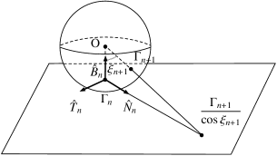
Figure 3: The Frenet frame for the curves on sphere.

For example, let $\xi_{n}=\xi$ and $a>0$ be constants, and we define the deformation of the Frenet frame by

$$\dot{F}_{n}=F_{n}M_{n},\quad M_{n}=\frac{1}{a}\left[\begin{array}[]{ccc}\vskip 3.0pt plus 1.0pt minus 1.0pt0&-\cos\xi\tan\frac{\hat{\kappa}_{n}}{2}-\tan\frac{\hat{\kappa}_{n+1}}{2}&-\sin\xi\tan\frac{\hat{\kappa}_{n}}{2}\\ \vskip 3.0pt plus 1.0pt minus 1.0pt\cos\xi\tan\frac{\hat{\kappa}_{n}}{2}+\tan\frac{\hat{\kappa}_{n+1}}{2}&0&-\sin\xi\\ \sin\xi\tan\frac{\hat{\kappa}_{n}}{2}&\sin\xi&0\end{array}\right],$$ (A.22)

then it follows from the compatibility condition of (A.21) and (A.22) the semi-discrete mKdV equation for $\hat{\kappa}_{n}$

$$\dot{\hat{\kappa}}_{n}=\dfrac{\,1\,}{a}\left(\tan\dfrac{\hat{\kappa}_{n+1}}{2}-\tan\dfrac{\hat{\kappa}_{n-1}}{2}\right).$$ (A.23)

To derive the deformation for the curve $\Gamma_{n}$, since we have $\hat{B}_{n}=-\lambda\Gamma_{n}$ from (A.20), the third column of the matrices in both sides of (A.22) immediately yields

$$\dot{\Gamma}_{n}=\frac{1}{a\lambda}\left(\sin\xi\tan\frac{\hat{\kappa}_{n}}{2}\,\hat{T}_{n}+\sin\xi\,\hat{N}_{n}\right).$$ (A.24)

This is the deformation of the discrete curves on sphere which is analogous to the deformation of the discrete space curves discussed in Section 5. In order to transform it to the deformation of the curve $\gamma_{n}$ in $\mathbb{R}^{3}$ by using the correspondence in (A.12), it is necessary to perform the summation, which is not a trivial procedure.

References

- [1] M.J. Ablowitz, D.J. Kaup, A.C. Newell and H. Segur, The inverse scattering transform-Fourier analysis for nonlinear problems, Studies in Appl. Math.53(1974) 249–315.
- [2] L.M. Bates and O.M. Melko, On curves of constant torsion I, J. Geom. 104(2013)213–227.
- [3] A. Bobenko and U. Pinkall, Discrete surfaces with constant negative Gaussian curvature and the Hirota equation, J. Diff. Geom. 43(1996) 527-611.
- [4] A.I. Bobenko and Y.B. Suris, Discrete Differential Geometry (American Mathematical Society, Providence, RI, 2008).
- [5] A. Calini and T. Ivey, Bäcklund transformations and knots of constant torsion, J. Knot Theory Ramifications 7 (1998) 719–746.
- [6] A. Doliwa and P.M. Santini, An elementary geometric characterization of the integrable motions of a curve, Phys. Lett. A185(1994) 373–384.
- [7] A. Doliwa and P.M. Santini, Integrable dynamics of a discrete curve and the Ablowitz-Ladik hierarchy, J. Math. Phys. 36(1995) 1259–1273.
- [8] A. Doliwa and P. M. Santini, The integrable dynamics of a discrete curve, Symmetries and Integrability of Difference Equations, D. Levi, L. Vinet and P. Winternitz (eds.), CRM Proceedings & Lecture Notes Vol.9 (American Mathematical Society, Providence, RI, 1996) 91–102.
- [9] H. Eyring, The resultant electric moment of complex molecules, Phys. Rev. 39(1932) 746–748.
- [10] R. E. Goldstein and D. M. Petrich, The Korteweg-de Vries hierarchy as dynamics of closed curves in the plane, Phys. Rev. Lett. 67 (1991) 3203–3206.
- [11] H. Hasimoto, A soliton on a vortex filament, J. Fluid. Mech. 51(1972) 477–485.
- [12] R. Hirota, Nonlinear partial difference equations III; discrete sine-Gordon equation, J. Phys. Soc. Jpn. 43 (1977) 2079-2086 .
- [13] M. Hisakado, K. Nakayama and M. Wadati, Motion of discrete curves in the plane, J. Phys. Soc. Jpn. 64 (1995) 2390–2393.
- [14] M. Hisakado and M. Wadati, Moving discrete curve and geometric phase, Phys. Lett. A214(1996) 252–258.
- [15] T.Hoffmann, Discrete Hashimoto surfaces and a doubly discrete smoke-ring flow, Discrete Differential Geometry, A.I. Bobenko, P. Schröder, J.M. Sullivan and G.M. Ziegler (eds.), Oberwolfach Seminars Vol.38 (Birkhäuser, Basel, 2008) 95–115.
- [16] T. Hoffmann, Discrete Differential Geometry of Curves and Surfaces, COE lecture Notes Vol. 18 (Kyushu University, Fukuoka, 2009).
- [17] T. Hoffmann and N. Kutz, Discrete curves in and the Toda lattice, Stud. Appl. Math. 113 (2004) 31–55.
- [18] J. Inoguchi, K. Kajiwara, N. Matsuura and Y. Ohta, Motion and Bäcklund transformations of discrete plane curves, Kyushu J. Math. 66(2012) 303–324.
- [19] J. Inoguchi, K. Kajiwara, N. Matsuura and Y. Ohta, Explicit solutions to the semi-discrete modified KdV equation and motion of discrete plane curves, J. Phys. A: Math. Theor. 45(2012) 045206.
- [20] G. Koenigs, Sur la forme des courbes à torsion constante, Ann. Fac. Sci. Toulouse Math. 1(1887) 1-8.
- [21] G.L. Lamb Jr., Solitons and the motion of helical curves, Phys. Rev. Lett. 37(1976) 235–237.
- [22] J. Langer and R. Perline, Curve motion inducing modified Korteweg-de Vries systems, Phys. Lett. A239(1998) 36–40.
- [23] N. Matsuura, Discrete KdV and discrete modified KdV equations arising from motions of planar discrete curves, Int. Math. Res. Not. 2012(2012) 1681–1698.
- [24] K. Nakayama, Elementary vortex filament model of the discrete nonlinear Schrödinger equation, J. Phys. Soc. Jpn. 76(2007) 074003.
- [25] K. Nakayama, H. Segur and M. Wadati, Integrability and the motions of curves, Phys. Rev. Lett. 69(1992) 2603–2606.
- [26] K. Nishinari, A discrete model of an extensible string in three-dimensional space, J. Appl. Mech.66(1999) 695–701.
- [27] U. Pinkall, B. Springborn, and S. Weißmann, A new doubly discrete analogue of smoke ring flow and the real time simulation of fluid flow, J. Phys. A: Math. Theor. 40 (2007) 12563–12576.
- [28] C. Rogers and W.K. Schief, Bäcklund and Darboux Transformations: Geometry and Modern Applications in Soliton Theory (Cambridge University Press, Cambridge, 2002).
- [29] R. Sauer, Differenzengeometrie (Spring-Verlag, Berlin, 1970).
- [30] A. Sym, Soliton surfaces, Lett. Nuovo Cimento (2) 33(1982) 394–400.