Statistical properties of the energy exchanged between two heat baths coupled by thermal fluctuations

Abstract

We study both experimentally and theoretically the statistical properties of the energy exchanged between two electrical conductors, kept at different temperature by two different heat reservoirs, and coupled by the electric thermal noise. Such a system is ruled by the same equations as two Brownian particles kept at different temperatures and coupled by an elastic force. We measure the heat flowing between the two reservoirs, the thermodynamic work done by one part of the system on the other, and we show that these quantities exhibit a long time fluctuation theorem. Furthermore, we evaluate the fluctuating entropy, which satisfies a conservation law. These experimental results are fully justified by the theoretically analysis. Our results give more insight into the energy transfer in the famous Feymann ratchet widely studied theoretically but never in an experiment.

PACS:05.40.-a, 05.70.-a, 05.70.Ln

1 Introduction

In the study of the out-of-equilibrium dynamics of small systems (Brownian particles[1, 2, 3, 4], molecular motors [5], small devices [6], etc.) the role of thermal fluctuations is central. Indeed the thermodynamics variables, such as work, entropy and heat, fluctuate and the study of their statistical properties is important as it can provide several constrains on the system design and mechanisms[7, 8]. In recent years several experiments have analyzed systems in contact with a single heat bath and driven out of equilibrium by external forces [1, 2, 3, 4, 5, 6, 9, 10, 11]. On the other hand the important case in which the system is driven out of equilibrium by a temperature gradient and the energy exchanges are produced only by the thermal noise has been analyzed in many theoretical studies on model systems [12, 13, 14, 15, 16, 17, 18, 19] but only a few times in very recent experimental studies because of the intrinsic difficulties of dealing with large temperature differences in small systems [20, 21].

We report here an experimental and theoretical analysis of the energy exchanged between two conductors kept at different temperature and coupled by the electric thermal noise. This system is probably the simplest one to test recent ideas of stochastic thermodynamics, but in spite of its simplicity the interpretation of the observations proves far from elementary. We determine experimentally the heat flux, the out of equilibrium variance as functions of the temperature difference, and a conservation law for the fluctuating entropy, which we justify theoretically. We show that our system can be mapped into a mechanical one, where two Brownian particles are kept at different temperatures and coupled by an elastic force [14, 17, 19]. Thus our study gives more insight into the properties of the heat flux, produced by mechanical coupling, in the famous Feymann ratchet [22, 23] widely studied theoretically [14] but never in an experiment. Our results set strong constrains on the energy exchanged between coupled nano-systems kept at different temperature. Therefore our investigation has implications well beyond the simple system we consider here.
The system analyzed in this article is inspired by the proof developed by Nyquist [24], who gave, in 1928, a theoretical explanation of the measurements of Johnson [25] on the thermal noise voltage in conductors. Nyquist’s explanation is based on equilibrium thermodynamics and considers the power exchanged by two electrically coupled conductors, which are at same temperature $T$ in an adiabatic environment. Imposing the condition of thermal equilibrium he concluded correctly that the thermal noise voltage across a conductor of resistance $R$ has a power spectral density $|\tilde{\eta}_{\omega}|^{2}=4\ k_{B}\,T\,R$, i.e. the Nyquist noise formula where $k_{B}$ is the Boltzmann constant and $T$ the temperature of the conductor. Notice that, in 1928, many years before the proof of the fluctuation dissipation theorem (FDT), this was the second example, after the Einstein relation for Brownian motion, relating the dissipation of a system to the amplitude of the thermal noise. Specifically, in the Einstein relation it is the viscosity of the fluid which is related to the variance of the Brownian particles positions, whereas in the Nyquist equation it is the variance of the voltage across the conductor which is proportional to its resistance. Surprisingly, since 1928 nobody has analyzed the consequences of keeping the two resistances, used in the Nyquist’s proof, at two different temperatures, when the Nyquist’s equilibrium condition cannot be used. One is thus interested in measuring the statistical properties of the energy exchanged between the two conductors via the electric coupling of the two thermal noises. In this article we address this question both experimentally and theoretically and show the analogy with two Brownian particles kept at different temperatures and coupled by an elastic force. The key feature in the system we consider, is that the coupling between the two reservoirs is obtained only by either electrical or mechanical thermal fluctuations.

In a recent letter [20] we presented several experimental results and we briefly sketched the theoretical analysis concerning the system we consider in the present paper. In this extended article we want to give a full description of the theoretical analysis and present new experimental results and the details of the calibration procedure.

The paper is organized as follows: in section 2 we describe the experimental apparatus and the stochastic equations governing the relevant dynamic and thermodynamic quantities. We also discuss the analogy with two coupled Brownian particles. In section 3 we develop the theoretical analysis on the fluctuations of the different forms of energy flowing across the system, and discuss the corresponding fluctuation theorems. In section 4 we discuss the data analysis and the main experimental results on fluctuation theorems. Furthermore, we show experimental data confirming the validity of an entropy conservation law holding at any time. Finally we conclude in section 5.

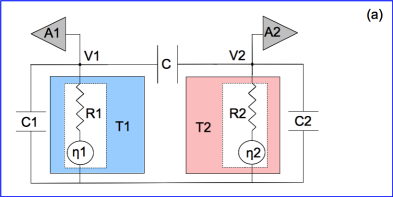
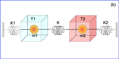
Figure 1: a) Diagram of the circuit. The resistances $R_{1}$ and $R_{2}$ are kept at temperature $T_{1}$ and $T_{2}=296K$ respectively. They are coupled via the capacitance $C$. The capacitances $C_{1}$ and $C_{2}$ schematize the capacitance of the cables and of the amplifier inputs. The voltages $V_{1}$ and $V_{2}$ are amplified by the two low noise amplifiers $A_{1}$ and $A_{2}$ [26]. b) The circuit in a) is equivalent to two Brownian particles ($m_{1}$ and $m_{2}$) moving inside two different heat baths at $T_{1}$ and $T_{2}$. The two particles are trapped by two elastic potentials of stiffness $K_{1}$ and $K_{2}$ and coupled by a spring of stiffness $K$ (see text and eqs.1,2).

2 Experimental set-up and stochastic variables

Our experimental set-up is sketched in fig.1a). It is constituted by two resistances $R_{1}$ and $R_{2}$, which are kept at different temperature $T_{1}$ and $T_{2}$ respectively. These temperatures are controlled by thermal baths and $T_{2}$ is kept fixed at $296K$ whereas $T_{1}$ can be set at a value between $296K$ and $88K$ using the stratified vapor above a liquid nitrogen bath. In the figure, the two resistances have been drawn with their associated thermal noise generators $\eta_{1}$ and $\eta_{2}$, whose power spectral densities are given by the Nyquist formula $|\tilde{\eta}_{m}|^{2}=4k_{B}R_{m}T_{m}$, with $m=1,2$ (see eqs. (1)-(2) ). The coupling capacitance $C$ controls the electrical power exchanged between the resistances and as a consequence the energy exchanged between the two baths. No other coupling exists between the two resistances which are inside two separated screened boxes. The quantities $C_{1}$ and $C_{2}$ are the capacitances of the circuits and the cables. Two extremely low noise amplifiers $A_{1}$ and $A_{2}$ [26] measure the voltage $V_{1}$ and $V_{2}$ across the resistances $R_{1}$ and $R_{2}$ respectively. All the relevant quantities considered in this paper can be derived by the measurements of $V_{1}$ and $V_{2}$, as discussed below.

2.1 Stochastic equations for the voltages

We now proceed to derive the equations for the dynamical variables $V_{1}$ and $V_{2}$. Furthermore, we will discuss how our system can be mapped onto a system with two interacting Brownian particles, in the overdamped regime, coupled to two different temperatures, see fig. 1-b). Let $q_{m}$ ($m=1,2$) be the charges that have flowed through the resistances $R_{m}$, so the instantaneous current flowing through them is $i_{m}=\dot{q}_{m}$. A circuit analysis shows that the equations for the charges are:

$$R_{1}\dot{q}_{1} = -q_{1}\,{C_{2}\over X}+(q_{2}-q_{1}){C\over X}+\eta_{1}$$ (1)

$$R_{2}\dot{q}_{2} = -q_{2}\,{C_{1}\over X}+(q_{1}-q_{2}){C\over X}+\eta_{2}$$ (2)

where $\eta_{m}$ is the usual white noise: $\left<{\eta_{i}(t)\eta_{j}(t^{\prime})}\right>=2\delta_{ij}{k_{B}T_{i}R_{j}}\delta(t-t^{\prime})$, and where we have introduced the quantity $X=C_{2}\,C_{1}+C\,(C_{1}\,+C_{2})$. Eqs. 1 and 2 are the same of those for the two coupled Brownian particles sketched in fig.1b) when one regards $q_{m}$ as the displacement of the particle $m$, $i_{m}$ as its velocity, $K_{m}=1/C_{m}$ as the stiffness of the spring $m$, $K=1/C$ as the coupling spring and $R_{m}$ the viscosity. The analogy with the Feymann ratchet can be made by assuming as done in ref.[14] that the particle $m_{1}$ has an asymmetric shape and on average moves faster in one direction than in the other one.

We now rearrange eqs. (1)-(2) to obtain the Langevin equations for the voltages, which will be useful in the following discussion. The relationships between the measured voltages and the charges are:

$$q_{1} = (V_{1}-V_{2})\,C+V_{1}\,C_{1}$$ (3)

$$q_{2} = (V_{1}-V_{2})\,C-V_{2}\,C_{2}.$$ (4)

By plugging eqs. (3)-(4) into eqs.(1)-(2), and rearranging terms, we obtain

$$(C_{1}+C)\dot{V}_{1} = C\dot{V}_{2}+\frac{1}{R_{1}}(\eta_{1}-V_{1}),$$ (5)

$$(C_{2}+C)\dot{V}_{2} = C\dot{V}_{1}+\frac{1}{R_{2}}(\eta_{2}-V_{2}).$$ (6)

We rearrange these equations in a standard form, and obtain

$$\dot{V}_{1} = f_{1}(V_{1},V_{2})+\sigma_{11}\eta_{1}+\sigma_{12}\eta_{2}=f_{1}(V_{1},V_{2})+\xi_{1}$$ (7)

$$\dot{V}_{2} = f_{2}(V_{1},V_{2})+\sigma_{21}\eta_{1}+\sigma_{22}\eta_{2}=f_{2}(V_{1},V_{2})+\xi_{2}$$ (8)

where the “forces” acting on the circuits read

$$f_{1}(V_{1},V_{2}) = -\left[{\frac{(C+C_{2})V_{1}}{R_{1}X}+\frac{CV_{2}}{R_{2}X}}\right],$$ (9)

$$f_{2}(V_{1},V_{2}) = -\left[{\frac{CV_{1}}{R_{1}X}+\frac{(C+C_{1})V_{2}}{R_{2}X}}\right],$$ (10)

the coefficients $\sigma_{ij}$ read

$$\sigma_{11} = \frac{C_{2}+C}{XR1}$$

$$R_{2}\sigma_{12} = R_{1}\sigma_{21}=\frac{C}{X}$$

$$\sigma_{22} = \frac{C_{1}+C}{XR_{2}},$$

and the noises $\xi_{i}$ introduced in eqs. (7)-(8) are now correlated $\left<{\xi_{i}\xi^{\prime}_{j}}\right>=2\theta_{ij}\delta(t-t^{\prime})$, where

$$\theta_{11} = \frac{k_{B}T_{1}(C_{2}+C)^{2}}{R_{1}X^{2}}+\frac{k_{B}T_{2}C^{2}}{R_{2}X^{2}},$$ (11)

$$\theta_{12} = \frac{k_{B}T_{1}C(C_{2}+C)}{R_{1}X^{2}}+\frac{k_{B}T_{2}C(C_{1}+C)}{R_{2}X^{2}},$$ (12)

$$\theta_{22} = \frac{k_{B}T_{1}C^{2}}{R_{1}X^{2}}+\frac{k_{B}T_{2}(C_{1}+C)^{2}}{R_{2}X^{2}},$$ (13)

and $\theta_{12}=\theta_{21}$.

2.2 Stochastic equations for work and heat exchanged between the two circuits

Two important quantities can be identified in the circuit depicted in fig. 1: the electric power dissipated in each resistor, and the work exerted by one circuit on the other one. We start by considering the first quantity $Q_{m}$, defined through the dissipation rate $\dot{Q}_{m}=V_{m}i_{m}$, where $i_{m}$ is the current flowing in the resistance $m$. As the voltages $V_{m}$ can be measured, one can obtain the currents as $i_{m}=i_{C}-i_{C_{m}}$, where

$$i_{C}=C\left({\dot{V}_{2}-\dot{V}_{1}}\right),\qquad i_{C_{m}}=C_{m}\dot{V}_{m},$$ (14)

are the current flowing in the capacitance $C$ and in $C_{m}$, respectively. Thus the total energy dissipated by the resistance $m$ in a time interval $\tau$ reads

$$Q_{m,\tau}=\int_{t_{0}}^{t_{0}+\tau}i_{m}(t)V_{m}(t)\mathrm{d}t=\int_{t_{0}}^{t_{0}+\tau}V_{m}\left[{C\dot{V}_{m^{\prime}}-(C_{m}+C)\dot{V}_{m}}\right]\mathrm{d}t,$$ (15)

We see that in equation (15) we can isolate the term $CV_{m}\dot{V}_{m^{\prime}}\mathrm{d}t$, denoting the work rate done by one circuit on the other one, from which we obtain the integrated quantities

$$W_{m,\tau}=\int_{t_{0}}^{t_{0}+\tau}CV_{m}(t)\dot{V}_{m^{\prime}}(t)\mathrm{d}t.$$ (16)

and

$$\Delta U_{m,\tau}={1\over 2}(C_{m}+C)(V_{m}^{2}(t+\tau)-V_{m}^{2}(t)$$ (17)

The quantities $W_{m,\tau}$ can be thus identified as the thermodynamic work performed by the circuit $m^{\prime}$ on $m$ [27, 28, 29]. As the two variables $V_{m}$ are fluctuating voltages, the derived quantities $Q_{m,\tau}$ and $W_{m,\tau}$ fluctuate too.

By plugging eqs. (7)-(8) into the definitions of dissipated energy and work, eqs. (15) and (16), respectively, we obtain the Langevin equations governing the time evolution of the two thermodynamic quantities:

$$\dot{W}_{m} = CV_{m}\dot{V}_{m^{\prime}}=CV_{m}(f_{m^{\prime}}+\xi_{m^{\prime}}),$$ (18)

$$\dot{Q}_{m} = V_{m}i_{m}=V_{m}\left[{C\dot{V}_{m^{\prime}}-(C_{m}+C)\dot{V}_{m}}\right]=\frac{V_{m}}{R_{m}}(V_{m}-\eta_{m}).$$ (19)

It is instructive to reconsider the quantity $Q_{m,\tau}$ in terms of the stochastic energetics [7]. If we introduce the circuit total potential energy, defined as

$$U=\frac{C_{1}}{2}V_{1}^{2}+\frac{C}{2}(V_{1}-V_{2})^{2}+\frac{C_{2}}{2}V_{2}^{2}=\frac{C_{2}q_{1}^{2}+C(q1-q2)^{2}+C_{1}q_{2}^{2}}{2X},$$ (20)

by noticing that eqs.(1)-(2) can be written as $R_{m}\dot{q}_{m}=-\partial_{q_{m}}U+\eta_{m}$, and following Sekimoto [7] we see that we can write the dissipated energy as

$$Q_{m,\tau}=-\int_{t_{0}}^{t_{0}+\tau}\frac{\partial U}{\partial q_{m}}\mathrm{d}q_{m}=\int_{t_{0}}^{t_{0}+\tau}\frac{V_{m}}{R_{m}}(V_{m}-\eta_{m})\mathrm{d}t,$$ (21)

where we have expressed the charges in terms of the voltages by inverting eqs. (3)-(4). With the analogy of the Brownian particles, depicted in fig. 1-b), we see that our definition of dissipated energy $Q_{m}$ corresponds exactly to the work performed by the viscous forces and by the bath on the particle $m$, and it is consistent with the stochastic thermodynamics definition [7, 8, 19, 27, 28, 29, 30]. Thus, the quantity $Q_{1,\tau}$ ($Q_{2,\tau}$) can be interpreted as the heat flowing from the reservoir 2 to the reservoir 1 (from 1 to 2), in the time interval $\tau$, as an effect of the temperature difference.

Hence we have derived the set of Langevin equations, describing the time evolution of the dynamical variables for $V_{m}$, and of the thermodynamic variables $Q_{m}$ and $W_{m}$. One expects that both these thermodynamic quantities satisfy a fluctuation theorem (FT) of the type [13, 15, 19, 30, 31, 32]

$$\ln{P(E_{m,\tau})\over P(-E_{m,\tau})}=\beta_{12}\ E_{m,\tau}\Sigma(\tau)$$ (22)

where $E_{m,\tau}$ stands either for $W_{m,\tau}$ or $Q_{m,\tau}$, $\beta_{12}=(1/T_{1}-1/T_{2})/k_{B}$ and $\Sigma(\tau)\rightarrow 1$ for $\tau\rightarrow\infty$. In order to prove this relation, we need to discuss the statistics of the fluctuations of the quantity of interests, namely $V_{m}$, $W_{m}$, and $Q_{m}$.

3 Fluctuations of $V_{m}$, $W_{m}$ and $Q_{m}$

3.1 Probability distribution function for the voltages

We now study the joint probability distribution function (PDF) $P(V_{1},V_{2},t)$, that the system at time $t$ has a voltage drop $V_{1}$ across the resistor $R_{1}$ and a voltage drop $V_{2}$ across the resistor $R_{2}$. As the time evolution of $V_{1}$ and $V_{2}$ is described by the Langevin equations (7)-(8), it can be proved that the time evolution of $P(V_{1},V_{2},t)$ is governed by the Fokker-Planck equation [33]

$$\partial_{t}P(V_{1},V_{2},t) = L_{0}P(V_{1},V_{2},t)=-\frac{\partial}{\partial V_{1}}\left({f_{1}P}\right)-\frac{\partial}{\partial V_{2}}\left({f_{2}P}\right)+2\theta_{12}\frac{\partial^{2}}{\partial V_{1}\partial V_{2}}P$$ (23)

$$\qquad\qquad\qquad+\theta_{11}\frac{\partial^{2}}{\partial V_{1}^{2}}P+\theta_{22}\frac{\partial^{2}}{\partial V_{2}^{2}}P$$

We are interested in the long time steady state solution of eq. (23), which is time independent $P(V_{1},V_{2},t\rightarrow\infty)=P_{ss}(V_{1},V_{2})$. As the deterministic forces in eqs. (7)-(8) are linear in the variables $V_{1}$ and $V_{2}$, such a steady state solution reads

$$P_{ss}(V_{1},V_{2})=\frac{\pi\mathrm{e}^{-m_{ij}V_{i}V_{j}}}{\sqrt{\det\mathbf{m}}},$$ (24)

where the sum over repeated indices is understood, and where the $\mathbf{m}$ matrix entries read

$$m_{11} = \frac{Y\left[T_{2}(C+C_{1})Y+C^{2}R_{2}(T_{1}-T_{2})\right]}{2k_{B}\left[{Y^{2}T_{1}T_{2}+C^{2}R_{1}R_{2}(T_{1}-T_{2})^{2}}\right]},$$

$$m_{12} = m_{21}=-\frac{YC[(C_{2}+C)R_{2}T_{1}+(C_{1}+C)R_{1}T_{2}]}{2k_{B}\left[{Y^{2}T_{1}T_{2}+C^{2}R_{1}R_{2}(T_{1}-T_{2})^{2}}\right]},$$

$$m_{22} = \frac{Y\left[T_{1}(C+C_{2})Y-C^{2}R_{1}(T_{1}-T_{2})\right]}{2k_{B}\left[{Y^{2}T_{1}T_{2}+C^{2}R_{1}R_{2}(T_{1}-T_{2})^{2}}\right]},$$

where we have introduced the quantity $Y=\left[{(C_{1}+C)R_{1}+(C_{2}+C)R_{2}}\right]$.

Such a solution can be obtained by replacing eq. (24) into eq. (23), and by imposing the steady state condition $\partial_{t}P=0$. We are furthermore interested in the unconstrained steady state probabilities $P_{1,ss}(V_{1})$, and $P_{2,ss}(V_{2})$, which are obtained as follows

$$P_{1,ss}(V_{1}) = \int\mathrm{d}V_{2}P_{ss}(V_{1},V_{2})=\frac{\mathrm{e}^{-\frac{V_{1}^{2}}{2\sigma_{1}^{2}}}}{\sqrt{2\pi\sigma_{1}^{2}}}$$ (25)

$$P_{2,ss}(V_{2}) = \int\mathrm{d}V_{1}P_{ss}(V_{1},V_{2})=\frac{\mathrm{e}^{-\frac{V_{2}^{2}}{2\sigma_{2}^{2}}}}{\sqrt{2\pi\sigma_{2}^{2}}}$$ (26)

where the variances read

$$\sigma_{1}^{2} = k_{B}\frac{T_{1}(C+C_{2})Y+(T_{2}-T_{1})C^{2}R_{1}}{XY}$$ (27)

$$\sigma_{2}^{2} = k_{B}\frac{T_{2}(C+C_{1})Y-(T_{2}-T_{1})C^{2}R_{2}}{XY}$$ (28)

3.2 Average value and long time FT for $W_{1}$

In eqs. (15)-(16) $t_{0}$ denote the instant when one begins to measure the thermodynamic quantities. In the following we will assume that the system is already in a steady state at that time and take $t_{0}=0$ for simplicity. We will discuss the case of $W_{1}$ without loss of generality, the mathematical treatment for $W_{2}$ being identical. We first notice that the dynamics of $W_{1}$ is described by the Langevin equation (18): the noise affecting $W_{1}$ is $CV_{1}\xi_{2}$, which is thus correlated to the noises $\xi_{1},\,\xi_{2}$ affecting $V_{1}$ and $V_{2}$ through the diffusion matrix defined in eqs. (11)-(13). We introduce the joint probability distribution $\phi(V_{1},V_{2},W_{1},t)$: the time evolution of such a PDF is described by the Fokker-Planck equation

$$\partial_{t}\phi(V_{1},V_{2},W_{1},t) = -\frac{\partial}{\partial V_{1}}\left({f_{1}\phi}\right)-\frac{\partial}{\partial V_{2}}\left({f_{2}\phi}\right)+\theta_{11}\frac{\partial^{2}}{\partial V_{1}^{2}}\phi+\theta_{22}\frac{\partial^{2}}{\partial V_{2}^{2}}\phi$$ (29)

$$+2\theta_{12}\frac{\partial^{2}}{\partial V_{1}\partial V_{2}}\phi-C\frac{\partial}{\partial W_{1}}\left({V_{1}f_{2}\phi}\right)$$

$$+\theta_{12}C\left[{\frac{\partial}{\partial V_{1}}\left({V_{1}\frac{\partial}{\partial W_{1}}\phi}\right)+\frac{\partial}{\partial W_{1}}\left({V_{1}\frac{\partial}{\partial V_{1}}\phi}\right)}\right]$$

$$+2\theta_{22}C\frac{\partial}{\partial V_{2}}\left({V_{1}\frac{\partial}{\partial W_{1}}\phi}\right)+\theta_{22}(CV_{1})^{2}\frac{\partial^{2}}{\partial W_{1}^{2}}\phi.$$

We now introduce the generating function defined as $\psi(V_{1},V_{2},\lambda,t)=\int\mathrm{d}W_{1}\exp(\lambda W_{1})\phi(V_{1},V_{2},W_{1},t)$, whose dynamic is described by the Fokker-Planck equation

$$\partial_{t}\psi(V_{1},V_{2},\lambda,t)=\mathcal{L}_{\lambda}\psi,$$ (30)

where the operator $\mathcal{L}_{\lambda}$ reads

$$\mathcal{L}_{\lambda}\psi = -\frac{\partial}{\partial V_{1}}\left({f_{1}\psi}\right)-\frac{\partial}{\partial V_{2}}\left({f_{2}\psi}\right)+\theta_{11}\frac{\partial^{2}}{\partial V_{1}^{2}}\psi+\theta_{22}\frac{\partial^{2}}{\partial V_{2}^{2}}\psi+2\theta_{12}\frac{\partial^{2}}{\partial V_{1}\partial V_{2}}\psi$$ (31)

$$-\lambda\theta_{12}C\left[{\frac{\partial}{\partial V_{1}}\left({V_{1}\psi}\right)+\left({V_{1}\frac{\partial}{\partial V_{1}}\psi}\right)}\right]$$

$$-2\theta_{22}\lambda C\frac{\partial}{\partial V_{2}}\left({V_{1}\psi}\right)+\lambda CV_{1}(\theta_{22}\lambda CV_{1}+f_{2})\psi.$$

For the average value of the work, after a straightforward calculation, one finds

$$\partial_{t}\left<{W_{1}}\right> = \left[{\partial_{\lambda}\partial_{t}\int\mathrm{d}V_{1}\mathrm{d}V_{2}\psi(V_{1},V_{2},\lambda,t)}\right]_{\lambda=0}=\frac{C^{2}k_{B}(T_{2}-T_{1})}{XY},$$ (32)

As we are interested in the large time limit of the unconstrained generating function, we notice that $\int\mathrm{d}V_{1}\mathrm{d}V_{2}\psi(V_{1},V_{2},\lambda,t)\propto\exp\left[{t\mu_{0}(\lambda)}\right]$, where $\mu_{0}(\lambda)$ is the largest eigenvalue of the operator $\mathcal{L}_{\lambda}$. Thus, proving that the unconstrained PDF $P(W_{1},\tau)=\int\mathrm{d}V_{1}\mathrm{d}V_{2}\phi(V_{1},V_{2},W_{1},t)$ satisfies the FT (22) is equivalent to prove that $\mu_{0}(\lambda)$ exhibits the following symmetry:

$$\mu_{0}(\lambda)=\mu_{0}(-\lambda-\beta_{12}).$$ (33)

In order to prove such an equality, following [19] we introduce the operator

$$\tilde{\mathcal{L}}_{\lambda}=\mathrm{e}^{H}\mathcal{L}_{\lambda}\mathrm{e}^{-H},$$ (34)

where $H(V_{1},V_{2})$ is some dimensionless Hamiltonian to be determined: thus this transformation corresponds to a “rotation” of the operator $\mathcal{L}_{\lambda}$, or more precisely $\tilde{\mathcal{L}}_{\lambda}$ and $\mathcal{L}_{\lambda}$ are related by a unitary transformation.

Let’s consider an eigenvector $\psi_{n}(V_{1},V_{2},\lambda)$ of the original operator $\mathcal{L}_{\lambda}$, with eigenvalue $\mu_{n}(\lambda)$, then one easily finds that the following equality holds

$$\tilde{\mathcal{L}}_{\lambda}\mathrm{e}^{H}\psi_{n}(V_{1},V_{2},\lambda)=\mathrm{e}^{H}\mathcal{L}_{\lambda}\mathrm{e}^{-H}\mathrm{e}^{H}\psi(V_{1},V_{2},\lambda)=\mu_{n}(\lambda)\mathrm{e}^{H}\psi(V_{1},V_{2},\lambda),$$ (35)

thus, $\mathcal{L}_{\lambda}$ and $\tilde{\mathcal{L}}_{\lambda}$ have the same eigenvalues, only the eigenvectors are “rotated” by the operator $\exp(H)$. Note that eq. (35) holds for any choice of $H$.

Our goal is still to prove eq. (33). By choosing

$$H=\frac{C_{1}+C}{2k_{B}T_{1}}V_{1}^{2}-\frac{C}{k_{B}T_{2}}V_{1}V_{2}+\frac{C_{2}+C}{2k_{B}T_{2}}V_{2}^{2}.$$ (36)

one finds that the following equality holds

$$\tilde{\mathcal{L}}_{\lambda}=\mathcal{L}^{*}_{-\lambda-\beta_{12}},$$ (37)

where $\mathcal{L}^{*}_{\lambda}$ is the adjoint operator of $\mathcal{L}_{\lambda}$. From the above discussion we know that $\mathcal{L}_{\lambda}$ and $\tilde{\mathcal{L}}_{\lambda}$ have the same eigenvalues, while eq. (37) shows that $\tilde{\mathcal{L}}_{\lambda}$ and $\mathcal{L}^{*}_{-\lambda-\beta_{12}}$ are the same operator, and so that $\mathcal{L}_{\lambda}$ and $\mathcal{L}^{*}_{-\lambda-\beta_{12}}$ have the same spectra of eigenvalues, and in particular identical maximal eigenvalues. Thus we conclude that $\mu_{0}(\lambda)=\mu_{0}(-\lambda-\beta_{12})$, which is the FT (22) in the form of eq. (33).

3.3 Average value and long time FT for $Q_{m}$

We now consider the dissipated heat, defined through its time derivative, as given by eq. (19). Similarly to what we have done for $W_{1}$, we now introduce the joint PDF $\pi(V_{1},V_{2},Q_{1},t)$, and the corresponding generating function $\chi(V_{1},V_{2},\lambda,t)=\int\mathrm{d}Q_{1}\exp(\lambda Q_{1})\pi(V_{1},V_{2},Q_{1},t)$, obtaining the Fokker-Planck equation

$$\partial_{t}\chi(V_{1},V_{2},\lambda,t)=\mathcal{K}_{\lambda}\chi,$$ (38)

where the operator $\mathcal{K}_{\lambda}$ reads

$$\mathcal{K}_{\lambda}\chi = -\frac{\partial}{\partial V_{1}}\left({f_{1}\chi}\right)-\frac{\partial}{\partial V_{2}}\left({f_{2}\chi}\right)+\theta_{11}\frac{\partial^{2}}{\partial V_{1}^{2}}\chi+\theta_{22}\frac{\partial^{2}}{\partial V_{2}^{2}}\chi+2\theta_{12}\frac{\partial^{2}}{\partial V_{1}\partial V_{2}}\chi$$ (39)

$$+\lambda r_{11}\left[{\frac{\partial}{\partial V_{1}}\left({V_{1}\chi}\right)+\left({V_{1}\frac{\partial}{\partial V_{1}}\chi}\right)}\right]$$

$$+2\lambda r_{12}\frac{\partial}{\partial V_{2}}\left({V_{1}\chi}\right)+\lambda V_{1}^{2}\left({\lambda r_{22}+\frac{1}{R_{1}}}\right)\chi,$$

with

$$r_{11} = k_{1}\theta_{11}+k_{2}\theta_{12},$$

$$r_{12} = k_{1}\theta_{12}+k_{2}\theta_{22},$$

$$r_{22} = k_{1}^{2}\theta_{11}+k_{2}^{2}\theta_{22}+2k_{1}k_{2}\theta_{12},$$

and $k_{1}=(C_{1}+C)$, $k_{2}=-C$. Thus, after a straightforward calculation, we obtain the heat rate as given by

$$\partial_{t}\left<{Q_{1}}\right> = \left[{\partial_{\lambda}\partial_{t}\int\mathrm{d}V_{1}\mathrm{d}V_{2}\chi(V_{1},V_{2},\lambda,t)}\right]_{\lambda=0}=\frac{C^{2}k_{B}(T_{2}-T_{1})}{XY}.$$ (41)

The last result is identical to eq. (32), thus the averages of the two energies are equal $\left<{W_{1}(t)}\right>=\left<{Q_{1}(t)}\right>$. This can be easily understood by noticing that $Q_{m,\tau}$ and $W_{m,\tau}$ differ by a term proportional to $\int V_{m}\dot{V}_{m}\mathrm{d}t^{\prime}=\Delta V_{m}^{2}$, which vanishes on average in the steady state.

We can now relate the variance of $V_{1}$ and $V_{2}$ to the mean heat flux: using eq.(41) we can express eq. (27) and eq. (28) in the following way:

$$\sigma_{m}^{2} = \sigma_{m,\mathrm{eq}}^{2}+<\dot{Q}_{m}>R_{m}$$ (42)

where $\sigma_{m,\mathrm{eq}}^{2}=k_{B}T_{m}(C+C_{m^{\prime}})/X$ is the equilibrium value of $\sigma_{m}^{2}$, when $T_{m}=T_{m^{\prime}}$, and so $<\dot{Q}_{m}>=0$. Equation (42) represents an extension to the two temperatures case of the Harada-Sasa relation [35], which relates the difference of the equilibrium and out-of-equilibrium power spectra to the heat fluxes.

Following the same route described in section 3.2, we now want to prove the FT for the unconstrained heat distribution PDF $P(Q_{1},\tau)=\int\mathrm{d}V_{1}\mathrm{d}V_{2}\pi(V_{1},V_{2},Q_{1},t)$ satisfies the FT (22), which is equivalent to the requirement

$$\nu_{0}(\lambda)=\nu_{0}(\beta_{12}-\lambda),$$ (43)

where $\nu_{0}(\lambda)$ is the largest eigenvalue of the operator $\mathcal{K}_{\lambda}$, and so in the large time limit one expects $\int\mathrm{d}V_{1}\mathrm{d}V_{2}\chi(V_{1},V_{2},\lambda,t)\propto\exp\left[{\nu_{0}(\lambda)t}\right]$ . We introduce the transformation

$$\mathcal{\widetilde{K}}_{\lambda}=\mathrm{e}^{H}\mathcal{K}_{\lambda}\mathrm{e}^{-H},$$ (44)

where the “Hamiltonian” generator of the transformation reads $H=U/(k_{B}T_{2})$ and where $U$ is given by eq. (20). We then find, after a lengthy but straightforward calculation that $\mathcal{\widetilde{K}}_{\lambda}=\mathcal{K}_{\beta_{12}-\lambda}^{*}$ where $\mathcal{K}_{\lambda}^{*}$ is the adjoint operator of $\mathcal{K}_{\lambda}$. Thus we infer that $\mathcal{K}_{\lambda}$ and $\mathcal{K}_{\beta_{12}-\lambda}^{*}$ have the same spectra of eigenvalues, and in particular identical maximal eigenvalues, and so eq. (43) and the FT (22) follow.

4 Analysis of the experimental data

4.1 Experimental details

The electric systems and amplifiers are inside a Faraday cage and mounted on a floating optical table to reduce mechanical and acoustical noise. The resistance $R_{1}$, which is cooled by liquid Nitrogen vapors, changes of less than $0.1\%$ in the whole temperature range. Its temperature is measured by a PT1000 which is inside the same shield of $R_{1}$. The signal $V_{1}$ and $V_{2}$ are amplified by two custom designed JFET amplifiers [26] with an input current of $1pA$ and a noise of $0.7nV/\sqrt{Hz}$ at frequencies larger than $1Hz$ and increases at $8nV/\sqrt{Hz}$ at $0.1Hz$, see fig. 2. The resistances $R1$ and $R2$ have been used as input resistances of the amplifiers. The two signals $V_{1}$ and $V_{2}$ are amplified $10^{4}$ times and the amplifier outputs are filtered (at $4kHz$ to avoid aliasing) and acquired at $8kHz$ by 24 bits-ADC. We used different sets of $C_{1},C_{2}$ and $C$. The values of $C1$ and $C2$ are essentially set by the input capacitance of the amplifiers and by the cable length $680pF<C1<780pF$ and $400pF<C_{2}<500pF$. Instead $C$ has been changed from $100pF$ to $1000pF$. In the following we will take $C=100pF,C_{1}=680pF,C_{2}=420pF$ and $R_{1}=R_{2}=10M\Omega$, if not differently stated. The longest characteristic time of the system is $Y=\left[{(C_{1}+C)R_{1}+(C_{2}+C)R_{2}}\right]$ which for the mentioned values of the parameters is : $Y=13\,$ms.

4.1.1 Check of the calibration

When $T_{1}=T_{2}=296K$ the system is in equilibrium and exhibits no net energy flux between the two reservoirs. This is indeed the condition imposed by Nyquist to prove his formula, and we use it to check all the values of the circuit parameters. Applying the Fluctuation-Dissipation-Theorem (FDT) to the circuit in fig.1a), one finds the Nyquist’s expression for the variance of $V_{1}$ and $V_{2}$ at equilibrium, which reads $\sigma_{m,\mathrm{eq}}^{2}(T_{m})={k_{B}T_{m}(C+C_{m^{\prime}})/X}$ with $X=C_{2}\,C_{1}+C\,(C_{1}\,+C_{2})$, $m^{\prime}=2$ if $m=1$ and $m^{\prime}=1$ if $m=2$. For example one can check that at $T_{1}=T_{2}=296$ K, using the above mentioned values of the capacitances and resistances, the predicted equilibrium standard deviations of $V_{1}$ and $V_{2}$ are $2.33\mu V$ and $8.16\mu V$ respectively. These are indeed the measured values with an accuracy better than $1\%$. The equilibrium spectra of $V_{1}$ and $V_{2}$ at $T_{1}=T_{2}$ used for calibration of the capacitances are:

$$Sp_{1}(\omega) = {4k_{B}T_{1}\,R_{1}[1+\omega^{2}(C^{2}R_{1}R_{2}+R_{2}^{2}(C_{2}+C)^{2})]\over(1-\omega^{2}\,X\,R_{1}R_{2})^{2}+\omega^{2}Y^{2}},$$ (45)

$$Sp_{2}(\omega) = {4k_{B}T_{2}\,R_{2}[1+\omega^{2}(C^{2}R_{1}R_{2}+R_{1}^{2}(C_{1}+C)^{2})]\over(1-\omega^{2}\,X\,R_{1}R_{2})^{2}+\omega^{2}Y^{2}}.$$ (46)

This spectra can be easily obtained by applying FDT to the circuit of fig.1.

The two computed spectra are compared to the measured ones in fig. 2a). This comparison allows us to check the values of the capacitances $C_{1}$ and $C_{2}$ which depend on the cable length. We see that the agreement between the prediction and the measured power spectra is excellent and the global error on calibration is of the order of $1\%$. This corresponds exactly to the case discussed by Nyquist in which the two resistances at the same temperature are exchanging energy via an electric circuit ($C$ in our case).

4.1.2 Noise spectrum of the amplifiers

The noise spectrum of the amplifiers $A_{1}$ and $A_{2}$ (Fig.1a), measured with a short circuit at the inputs, is plotted in fig.2a) and compared with the spectrum $Sp_{1}$ of $V_{1}$ at $T_{1}=88K$. We see that the useful signal is several order of magnitude larger than the amplifiers noise.

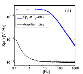
Figure 2: a) The power spectra $Sp_{1}$ of $V_{1}$ measured at $T_{1}=88K$ (blue line) ($C=100pF,C_{1}=680pF,C_{2}=430pF$) is compared to the spectrum of the amplifier noise. b) The equilibrium spectra $Sp_{1}$(red line) and $Sp_{2}$ (green line) measured at $T_{1}=T_{2}=296K$ are compared with prediction of eqs. (45) and (46) in order to check the values of the capacitances ($C_{1},C_{2}$).

4.2 The statistical properties of $V_{m}$

4.2.1 The power spectra and the variances of $V_{m}$ out-of-equilibrium

When $T_{1}\neq T_{2}$ the power spectra of $V_{1}$ and $V_{2}$ are:

$$Sp_{1}(\omega) = {4k_{B}T_{1}\,R_{1}[1+\omega^{2}(C^{2}R_{1}R_{2}+R_{2}^{2}(C_{2}+C)^{2})]\over(1-\omega^{2}\,X\,R_{1}R_{2})^{2}+\omega^{2}Y^{2}}+{4k_{B}(T_{2}-T_{1})\,\omega^{2}\,C^{2}R_{1}^{2}R_{2}\over(1-\omega^{2}\,X\,R_{1}R_{2})^{2}+\omega^{2}Y^{2}}$$ (47)

$$Sp_{2}(\omega) = {4k_{B}T_{2}\,R_{2}[1+\omega^{2}(C^{2}R_{1}R_{2}+R_{1}^{2}(C_{1}+C)^{2})]\over(1-\omega^{2}\,X\,R_{1}R_{2})^{2}+\omega^{2}Y^{2}}+{4k_{B}(T_{1}-T_{2})\,\omega^{2}\,C^{2}R_{2}^{2}R_{1}\over(1-\omega^{2}\,X\,R_{1}R_{2})^{2}+\omega^{2}Y^{2}}$$ (48)

These equations have been obtained by Fourier transforming the stochastic equations for the voltages eqs. (7)–(8), solving for $\tilde{V}_{1}(\omega)$ and $\tilde{V}_{2}(\omega)$ and computing the modula. The integral of eqs. (47) and (48) gives the variances of $V_{m}$ (as given by eq. (27)-(28)) directly computed from the distributions. Notice that the spectra eqs. (47) and (48) contains the equilibrium parts given by eqs. (45) and (46) and an out of equilibrium component proportional to the temperature difference. A comparison of eqs. (47)–(48) to the experimental power spectra is shown in fig. 3a). In fig. 3b) we compare the measured probability distribution function (PDF) of $V_{1}$ and $V_{2}$ with the equilibrium and the out-of-equilibrium distributions as computed by using the theoretical predictions eqs. (27)–(28) for the variance.

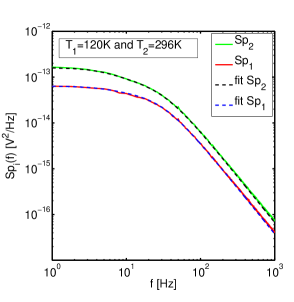
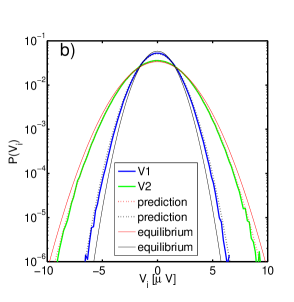
Figure 3: a) The power spectra $Sp_{1}$ of $V_{1}$ and $Sp_{2}$ of $V_{2}$ measured at $T_{1}=120K$ and $T_{2}=296K$ ($C=100pF,C_{1}=680pF,C_{2}=430pF$) are compared with the prediction of eq. (47) and (48) (dashed lines) The measured PDF of $V_{1}$ and $V_{2}$ are compared with the theoretical predictions in equilibrium and out of equilibrium obtained using the variance computed from eq. (42). b) The corresponding Probability Density Function $P(V_{1})$ of $V_{1}$ (green line) and $P(V_{2})$ of $V_{2}$ (blue line) measured at $T_{1}=120K$ and $T_{2}=296K$. Dotted lines are the out-of-equilibrium PDF, whose variance is estimated from the measure of the heat flux (see fig.5) and eq.42. The continuous red line is the equilibrium $P(V_{2})$ at $T_{1}=T_{2}=296K$ and the black continuous line corresponds to the equilibrium $P(V_{1})$ at $T_{1}=T_{2}=120K$.

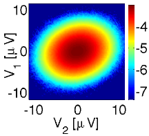
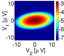
Figure 4: The joint probability $\log_{10}P(V_{1},V_{2})$ measured at $T_{1}=296K$ equilibrium (a) and out of equilibrium $T_{1}=88K$(b). The color scale is indicated on the colorbar on the right side.

4.2.2 The joint probability of $V_{1}$ and $V_{2}$

As discussed in sections 2 and 3, all the relevant thermodynamic quantities can be sampled once one has measured the voltage across the resistors $V_{1}$, $V_{2}$. The fluctuations of these quantities are thus to be fully characterized before one can proceed and study the fluctuations of all the derived thermodynamic quantities. Thus, we first study the joint probability distribution $P(V_{1},V_{2})$, which is plotted in fig. 4a) for $T_{1}=T_{2}$ and in fig. 4b) for $T_{1}=88K$. The fact that the axis of the ellipses defining the contours lines of $P(V_{1},V_{2})$ are inclined with respect to the $x$ and $y$ axis indicates that there is a certain correlation between $V_{1}$ and $V_{2}$. This correlation, produced by the electric coupling, plays a major role in determining the mean heat flux between the two reservoirs, as we discuss below. We are mainly interested in the out-of-equilibrium case, when $T_{1}\neq T_{2}$, and in the following, we will characterize the heat flux and the entropy production rate, and discuss how the variance of $V_{1}$ an $V_{2}$ are modified by the presence of a non-zero heat flux.

4.3 Heat flux fluctuations

In fig. 5a) we show the probability density function $P(Q_{1,\tau})$, at various temperatures: we see that $Q_{1,\tau}$ is a strongly fluctuating quantity, whose PDF $P(Q_{1,\tau})$ has long exponential tails. Notice that although for $T_{1}<T_{2}$ the mean value of $Q_{1,\tau}$ is positive, instantaneous negative fluctuations may occur, i.e., sometimes the heat flux is reversed. The mean values of the dissipated heat are expected to be linear functions of the temperature difference $\Delta T=T_{2}-T_{1}$, i.e. $\left<{Q_{1,\tau}}\right>=A\,\tau\,\Delta T$, where $A=k_{B}C^{2}/XY$ is a parameter dependent quantity, that can be obtained by eq. (41). This relation is confirmed by our experimental results, as shown in fig. 5b. Furthermore, the mean values of the dissipated heat satisfy the equality $\left<{Q_{2}}\right>=-\left<{Q_{1}}\right>$, corresponding to an energy conservation principle: the power extracted from the bath 2 is dissipated into the bath 1 because of the electric coupling.

As we discuss in section 3.3, the mean heat flow is related to a change in the variances $\sigma_{m}^{2}(T_{m})$ of $V_{m}$ with respect to the equilibrium value $\sigma_{m,\mathrm{eq}}^{2}(T_{m})$, see eq. (42). The experimental verification of eq. (42) is shown in the inset of fig. 5b) where the values of $\left<{\dot{Q}_{m}}\right>$ directly estimated from the experimental data (using the steady state $P(Q_{m})$) are compared with those obtained from the difference of the variances of $V_{1}$ measured in equilibrium and out-of-equilibrium. The values are comparable within the error bars and show that the out-of-equilibrium variances are modified only by the heat flux.

4.4 Fluctuation theorem for work and heat

As the system is in a stationary state, we have $\left<{W_{m,\tau}}\right>=\left<{Q_{\tau,m}}\right>$. Instead the comparison of the pdf of $W_{m,\tau}$ with those of $Q_{\tau,m}$, measured at various temperatures, presents several interesting features. In fig. 6(a) we plot $P(W_{1,\tau})$, $P(-W_{2,\tau})$, $P(Q_{1,\tau})$ and $P(-Q_{2,\tau})$ measured in equilibrium at $T_{1}=T_{2}=296K$ and $\tau\simeq 0.1s\simeq 10\,Y$. We immediately see that the fluctuations of the work are almost Gaussian whereas those of the heat presents large exponential tails. This well known difference [28] between $P(Q_{m,\tau})$ and $P(W{m,\tau})$ is induced by the fact that $Q_{m,\tau}$ depends also on $\Delta U_{m,\tau}$ (eq.17), which is the sum of the square of Gaussian distributed variables, thus inducing exponential tails in $P(Q_{m,\tau})$. In fig. 6(a) we also notice that $P(W_{1,\tau})=P(-W_{2,\tau})$ and $P(Q_{1,\tau})=P(-Q_{2,\tau})$, showing that in equilibrium all fluctuations are perfectly symmetric. The same pdfs measured in the out of equilibrium case at $T_{1}=88K$ are plotted in fig. 6(b). We notice here that in this case the behavior of the pdfs of the heat is different from those of the work. Indeed although $\left<{W_{m,\tau}}\right>>0$ we observe that $P(W_{1,\tau})=P(-W_{2,\tau})$, while $P(Q_{1,\tau})\neq P(-Q_{2,\tau})$. Indeed the shape of $P(Q_{1,\tau})$ is strongly modified by changing $T_{1}$ from $296K$ to $88K$, whereas the shape of $P(-Q_{2,\tau})$ is slightly modified by the large temperature change, only the tails of $P(-Q_{2,\tau})$ presents a small asymmetry testifying the presence of a small heat flux. The fact that $P(Q_{1,\tau})\neq P(-Q_{2,\tau})$ whereas $P(W_{1,\tau})=P(-W_{2,\tau})$ can be understood by noticing that $Q_{m,\tau}=W_{m,\tau}-\Delta U_{m,\tau}$. Indeed $\Delta U_{m,\tau}$ (eq.17) depends on the values of $C_{m}$ and $V_{m}^{2}$. As $C_{1}\neq C_{2}$ and $\sigma_{2}\geq\sigma_{1}$, this explains the different behavior of $Q_{1}$ and $Q_{2}$. Instead $W_{m}$ depends only on $C$ and the product $V_{1}\,V_{2}$.

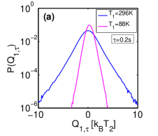
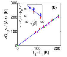
Figure 5: a) The probability $P(Q_{1,\tau})$ measured at $T_{1}=296K$ (blue line) equilibrium and $T_{1}=88K$ (magenta line) out of equilibrium. Notice that the peak of the $P(Q_{1,\tau})$ is centered at zero at equilibrium and shifted towards a positive value out of equilibrium. The amount of the shift is very small and is $\sim k_{B}(T_{2}-T_{1})$. b) The measured mean value of $\left<{Q_{1,\tau}}\right>$ is a linear function of $(T_{2}-T_{1})$. The red points correspond to measurements performed with the values of the capacitance $C_{1},C_{2},C$ given in the text and $\tau=0.2s$. The other symbols and colors pertain to different values of these capacitance and other $\tau$: (black $\circ$) $\tau=0.4s,C=1000pF$, (green $\triangleleft$) $\tau=0.1s,C=100pF$, (magenta $+$) $\tau=0.5s,C=100pF$. The values of $\left<{Q_{1,\tau}}\right>$ have been rescaled by the parameter dependent theoretical prefactor $A$, which allows the comparison of different experimental configurations. The continuous blue line with slope $1$ is the theoretical prediction of eq. 41. In the inset the values of $<\dot{Q}_{1}>$ (at $C=1000pF$) directly measured using $P(Q_{1})$ (blue square) are compared with those (red circles) obtained from the eq. (42).

We have studied whether our data satisfy the fluctuation theorem as given by eq. (22) in the limit of large $\tau$. It turns out that the symmetry imposed by eq. (22) is reached for rather small $\tau$ for $W$. Instead it converges very slowly for $Q$. We only have a qualitative argument to explain this difference in the asymptotic behavior: by looking at the data one understands that the slow convergence is induced by the presence of the exponential tails of $P(Q_{1,\tau})$ for small $\tau$.

To check eq. 22, we plot in fig. 6c) the symmetry function $Sym(E_{1,\tau})=\ln{P(E_{1,\tau})\over P(-E_{1,\tau})}$ as a function of $E_{1,\tau}/(k_{B}T_{2})$ measured at different $T_{1}$, but $\tau=0.1s$ for $Sym(W_{1,\tau})$ and $\tau=2s\simeq 200Y$ for $Sym(Q_{1,\tau})$. Indeed for $Sym(Q_{1,\tau})$ reaches the asymptotic regime only for $\tau<2s$. We see that $Sym(W_{1,\tau})$ is a linear function of $W_{1,\tau}/(k_{B}T_{2})$ at all $T_{1}$. These straight lines have a slope $\alpha(T_{1})$ which, according to eq.22 should be $(\beta_{12}k_{B}T_{2})$. In order to check this prediction we fit the slopes of the straight lines in fig.22c). From the fitted $\alpha(T_{1})$ we deduce a temperature $T_{fit}=T_{2}/(\alpha(T1)+1)$ which is compared to the measured temperature $T_{1}$ in fig.22d). In this figure the straight line of slope 1 indicates that $T_{fit}\simeq T_{1}$ within a few percent. These experimental results indicate that our data verify the fluctuation theorem, eq.22, for the work and the heat but that the asymptotic regime is reached for much larger time for the latter.

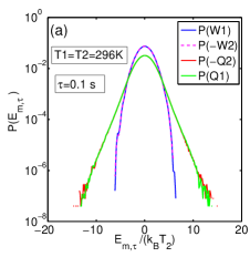
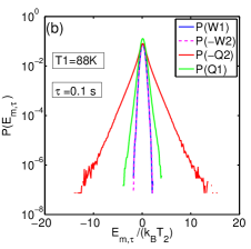
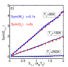
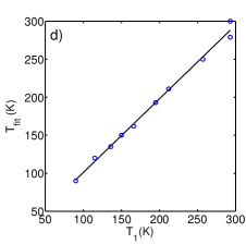
Figure 6: a) Equilibrium: $P(W_{m,\tau})$ and $P(Q_{m,\tau})$, measured in equilibrium at $T_{1}=T_{2}=296K$ and $\tau=0.1s$, are plotted as functions of $E$, where $E$ stands either for $W$ or $Q$. Notice that, being the system in equilibrium $P(W_{1,\tau})=P(-W_{2,\tau})$, $P(Q_{1,\tau})=P(-Q_{2,\tau})$. b) Out of equilibrium: same distributions as in a) but the PDFs are measured at $T_{1}=88K$, $T_{2}=296K$ and $\tau=0.1s$. Notice that in out of equilibrium $P(W_{1,\tau})=P(-W_{2,\tau})$ but $P(Q_{1,\tau})\neq P(-Q_{2,\tau})$. The reason of this difference is explained in the text. c) The symmetry function $Sym(E_{1,\tau})$, measured a various $T_{1}$ is plotted as a function of $E_{1}$ ($W_{1}$ or $Q_{1}$). The theoretical slope of these straight lines is $T_{2}/T_{1}-1$. d) The temperature $T_{fit}$ estimated from the slopes of the lines in c) is plotted as a function of the $T_{1}$ measured by the thermometer. The slope of the line is 1 showing that $T_{fit}\simeq T_{1}$ within a few percent.

4.5 Statistical properties of entropy

We now turn our attention to the study of the entropy produced by the total system, circuit plus heat reservoirs. We consider first the entropy $\Delta S_{r,\tau}$ due to the heat exchanged with the reservoirs, which reads $\Delta S_{r,\tau}=Q_{1,\tau}/T_{1}+Q_{2,\tau}/T_{2}$. This entropy is a fluctuating quantity as both $Q_{1}$ and $Q_{2}$ fluctuate, and its average in a time $\tau$ is $\left<{\Delta S_{r,\tau}}\right>=\left<{Q_{r,\tau}}\right>(1/T_{1}-1/T_{2})=A\tau(T_{2}-T_{1})^{2}/(T_{2}\,T_{1})$. However the reservoir entropy $\Delta S_{r,\tau}$ is not the only component of the total entropy production: one has to take into account the entropy variation of the system, due to its dynamical evolution. Indeed, the state variables $V_{m}$ also fluctuate as an effect of the thermal noise, and thus, if one measures their values at regular time interval, one obtains a “trajectory” in the phase space $(V_{1}(t),V_{2}(t))$. Thus, following Seifert [34], who developed this concept for a single heat bath, one can introduce a trajectory entropy for the evolving system $S_{s}(t)=-k_{B}\log P(V_{1}(t),V_{2}(t))$, which extends to non-equilibrium systems the standard Gibbs entropy concept. Therefore, when evaluating the total entropy production, one has to take into account the contribution over the time interval $\tau$ of

$$\Delta S_{s,\tau}=-k_{B}\log\left[{P(V_{1}(t+\tau),V_{2}(t+\tau))\over P(V_{1}(t),V_{2}(t))}\right].$$ (49)

It is worth noting that the system we consider is in a non-equilibrium steady state, with a constant external driving $\Delta T$. Therefore the probability distribution $P(V_{1},V_{2})$ (as shown in fig. 4b)) does not depend explicitly on the time, and $\Delta S_{s,\tau}$ is non vanishing whenever the final point of the trajectory is different from the initial one: $(V_{1}(t+\tau),V_{2}(t+\tau))\neq(V_{1}(t),V_{2}(t))$. Thus the total entropy change reads $\Delta S_{tot,\tau}=\Delta S_{r,\tau}+\Delta S_{s,\tau}$, where we omit the explicit dependence on $t$, as the system is in a steady-state as discussed above. This entropy has several interesting features. The first one is that $\left<{\Delta S_{s,\tau}}\right>=0$, and as a consequence $\left<{\Delta S_{tot}}\right>=\left<{\Delta S_{r}}\right>$ which grows with increasing $\Delta T$. The second and most interesting result is that independently of $\Delta T$ and of $\tau$, the following equality always holds:

$$\left<{\exp(-\Delta S_{tot}/k_{B})}\right>=1,$$ (50)

for which we find both experimental evidence, as discussed in the following, and provide a theoretical proof in appendix A. Equation (50) represents an extension to two temperature sources of the result obtained for a system in a single heat bath driven out-of-equilibrium by a time dependent mechanical force [34, 4] and our results provide the first experimental verification of the expression in a system driven by a temperature difference. Eq. (50) implies that $\left<{\Delta S_{tot}}\right>\,\geq 0$, as prescribed by the second law. From symmetry considerations, it follows immediately that, at equilibrium ($T_{1}=T_{2}$), the probability distribution of $\Delta S_{tot}$ is symmetric: $P_{eq}(\Delta S_{tot})=P_{eq}(-\Delta S_{tot})$. Thus Eq. (50) implies that the probability density function of $\Delta S_{tot}$ is a Dirac $\delta$ function when $T_{1}=T_{2}$, i.e. the quantity $\Delta S_{tot}$ is rigorously zero in equilibrium, both in average and fluctuations, and so its mean value and variance provide a measure of the entropy production. The measured probabilities $P(\Delta S_{r})$ and $P(\Delta S_{tot})$ are shown in fig. 7a). We see that $P(\Delta S_{r})$ and $P(\Delta S_{tot})$ are quite different and that the latter is close to a Gaussian and reduces to a Dirac $\delta$ function in equilibrium, i.e. $T_{1}=T_{2}=296K$ (notice that, in fig.7a, the small broadening of the equilibrium $P(\Delta S_{tot})$ is just due to unavoidable experimental noise and discretization of the experimental probability density functions). The experimental measurements satisfy eq. (50) as it is shown in fig. 7b). It is worth to note that eq. (50) implies that $P(\Delta S_{tot})$ should satisfy a fluctuation theorem of the form $\log[P(\Delta S_{tot})/P(-\Delta S_{tot})]=\Delta S_{tot}/k_{B},\,\,\,\forall\tau,\Delta T$, as discussed extensively in reference [8, 36]. We clearly see in fig.7c) that this relation holds for different values of the temperature gradient. Thus this experiment clearly establishes a relationship between the mean and the variance of the entropy production rate in a system driven out-of-equilibrium by the temperature difference between two thermal baths coupled by electrical noise. Because of the formal analogy with Brownian motion the results also apply to mechanical coupling as discussed in the following.

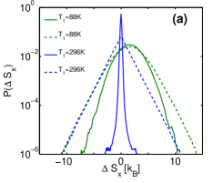
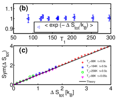
Figure 7: a) The probability $P(\Delta S_{r})$ (dashed lines) and $P(\Delta S_{tot})$ (continuous lines) measured at $T_{1}=296K$ (blue line) which corresponds to equilibrium and $T_{1}=88K$ (green lines) out of equilibrium. Notice that both distributions are centered at zero at equilibrium and shifted towards positive value in the out-of-equilibrium. b) $\left<{\exp(-\Delta S_{tot})}\right>$ as a function of $T_{1}$ at two different $\tau=0.5s$ and $\tau=0.1s$. c) Symmetry function $\rm{Sym}(\Delta S_{tot})=\log[P(\Delta S_{tot})/P(-\Delta S_{tot})]$ as a function of $\Delta S_{tot}$. The black straight line of slope 1 corresponds to the theoretical prediction.

5 Conclusions

We have studied experimentally and theoretically the statistical properties of the energy exchanged between two heat baths at different temperatures which are coupled by electric thermal noise. We have measured the heat flux, the thermodynamic work and the total entropy, and shown that each of these quantities exhibits a FT, in particular we have shown the existence of a conservation law for entropy which is not asymptotic in time. Our results hold in full generality since the electric system considered here is ruled by the same equations as for two Brownian particles, held at different temperatures and mechanically coupled by a conservative potential. Therefore these results set precise constraints on the energy exchanged between coupled nano and micro-systems held at different temperatures. Our system can be easily scaled to include more than two heat reservoirs, and more electric elements to mimic more complex dynamics in a system of Brownian particles. We thus believe that our study can represent the basis for further investigation in out-of-equilibrium physics.

Appendix A Entropy conservation law

We now turn our attention to eq. (2), in the main text, and provide a formal proof for it. In the present appendix we provide a formal proof of eq. (50). Let’s divide the time into small intervals $\Delta t$, and let $\mathbf{V}=(V_{1},V_{2})$ denote the system’s stat at time $t$, and $\mathbf{V}^{\prime}=(V_{1}+\Delta V_{1},V_{2}+\Delta V_{2})$ its state at time $t+\Delta t$. Let $\mathcal{P}_{F}(\mathbf{V}\rightarrow\mathbf{V}^{\prime}|\mathbf{V},t)$ be the probability that the system undergoes a transition from $\mathbf{V}$ to $\mathbf{V}^{\prime}$ provided that its state at time $t$ is $\mathbf{V}$, and let $\mathcal{P}_{R}(\mathbf{V}^{\prime}\rightarrow\mathbf{V}|\mathbf{V}^{\prime},t+\Delta t)$ be the probability of the time-reverse transition. By noticing that the time evolution of the dynamic variables $V_{m}$ is ruled by eqs. (7)-(8), we find that the probability of the forward trajectory can be written as

$$P_{F}(\mathbf{V}\rightarrow\mathbf{V}^{\prime}|\mathbf{V},t) = \int\mathrm{d}\eta_{1}\mathrm{d}\eta_{2}\,\delta(\Delta V_{1}-\Delta t\cdot(f1(V_{1},V_{2})+\sigma_{11}\eta_{1}+\sigma_{12}\eta_{2}))$$ (51)

$$\times\delta(\Delta V_{2}-\Delta t\cdot(f_{2}(V_{1},V_{2})+\sigma_{21}\eta_{1}+\sigma_{22}\eta_{2}))p_{1}(\eta_{1})p_{2}(\eta_{2}),$$

where $\delta(x)$ is the Dirac delta function, and $p_{m}(\eta_{m})$ is the probability distribution of the $m$-th Gaussian noise

$$p_{m}(\eta_{m})=\exp\left[{-\frac{\eta_{m}^{2}\Delta t}{4R_{m}k_{B}T}}\right]\sqrt{\frac{\Delta t}{4\pi R_{m}k_{B}T_{m}}}.$$ (52)

Expressing the Dirac delta in Fourier space $\delta(x)=1/(2\pi)\int\mathrm{d}q\exp(iqx)$, eq. (51) becomes

$$P_{F}(\mathbf{V}\rightarrow\mathbf{V}^{\prime}|\mathbf{V},t) = \int\frac{\mathrm{d}q_{1}\mathrm{d}q_{2}}{(2\pi)^{2}}\exp\left[{\imath(q_{1}\Delta V_{1}+q_{2}\Delta V_{2})}\right]\int\prod_{m}\mathrm{d}\eta_{m}\,\mathrm{e}^{\Delta t\left[{\imath q_{m}(f_{m}+\sigma_{m1}\eta_{1}+\sigma_{m2}\eta_{2})-\frac{\eta_{m}^{2}}{4R_{m}k_{B}T}}\right]}$$ (54)

$$= \exp\left\{-\frac{\Delta t}{4k_{B}T_{1}T_{2}}\left[C_{1}^{2}R_{1}T_{2}(\dot{V}_{1}-f_{1})^{2}+C_{2}^{2}R_{2}T_{1}(\dot{V}_{2}-f_{2})^{2}\right.\right.$$

$$\qquad+2C(\dot{V}_{1}-f_{1}-\dot{V}_{2}+f_{2})(C_{1}R_{1}T_{2}(\dot{V}_{1}-f_{1})-C_{2}R_{2}T_{1}(\dot{V}_{2}-f_{2}))$$

$$\qquad\left.\left.+C^{2}(R_{2}T_{1}+R_{1}T_{2})(\dot{V}_{1}-f_{1}-\dot{V}_{2}+f_{2})^{2}\right]\right\}\frac{X}{4\pi k_{B}\Delta t}\sqrt{\frac{R_{1}R_{2}}{T_{1}T_{2}}};$$

where we have taken $\Delta V_{m}/\Delta t\simeq\dot{V}_{m}$. A similar calculation for the reverse transition gives

$$P_{R}(\mathbf{V}^{\prime}\rightarrow\mathbf{V}|\mathbf{V}^{\prime},t+\Delta t) = \int\mathrm{d}\eta_{1}\mathrm{d}\eta_{2}\,\delta(\Delta V_{1}+\Delta t(f1(V_{1}^{\prime},V_{2}^{\prime})+\sigma_{11}\eta_{1}+\sigma_{12}\eta_{2}))$$ (56)

$$\times\delta(\Delta V_{2}+\Delta t(f_{2}(V_{1}^{\prime},V_{2}^{\prime})+\sigma_{21}\eta_{1}+\sigma_{22}\eta_{2}))p_{1}(\eta_{1})p_{2}(\eta_{2})$$

$$= \exp\left\{-\frac{\Delta t}{4k_{B}T_{1}T_{2}}\left[C_{1}^{2}R_{1}T_{2}(\dot{V}_{1}+f_{1})^{2}+C_{2}^{2}R_{2}T_{1}(\dot{V}_{2}+f_{2})^{2}\right.\right.$$

$$\qquad+2C(\dot{V}_{1}+f_{1}-\dot{V}_{2}-f_{2})(C_{1}R_{1}T_{2}(\dot{V}_{1}+f_{1})-C_{2}R_{2}T_{1}(\dot{V}_{2}+f_{2}))$$

$$\qquad\left.\left.+C^{2}(R_{2}T_{1}+R_{1}T_{2})(\dot{V}_{1}+f_{1}-\dot{V}_{2}-f_{2})^{2}\right]\right\}\frac{X}{4\pi k_{B}\Delta t}\sqrt{\frac{R_{1}R_{2}}{T_{1}T_{2}}}.$$

We now consider the ratio between the probability of the forward and backward trajectories, and by substituting the explicit definitions of $f_{1}(V_{1},V_{2})$ and $f_{2}(V_{1},V_{2})$, as given by eqs. (9)-(10), into eqs. (54) and (56), we finally obtain

$$\log\frac{P_{F}(\mathbf{V}\rightarrow\mathbf{V}^{\prime}|\mathbf{V},t)}{P_{R}(\mathbf{V}^{\prime}\rightarrow\mathbf{V}|\mathbf{V}^{\prime},t+\Delta t)}=-\Delta t\left({V_{1}\frac{(C_{1}+C)\dot{V}_{1}-C\dot{V}_{2}}{k_{B}T_{1}}+V_{2}\frac{(C_{2}+C)\dot{V}_{2}-C\dot{V}_{1}}{k_{B}T_{2}}}\right)=\Delta t\left({\frac{\dot{Q}_{1}}{k_{B}T_{1}}+\frac{\dot{Q}_{2}}{k_{B}T_{2}}}\right),$$ (57)

where we have exploited eq. (19) in order to obtain the rightmost equality. Thus, by taking a trajectory $\mathbf{V}\rightarrow\mathbf{V}^{\prime}$ over an arbitrary time interval $[t,t+\tau]$, and by integrating the right hand side of eq. (57) over such time interval, we finally obtain

$$k_{B}\log\frac{P_{F}(\mathbf{V}\rightarrow\mathbf{V}^{\prime}|\mathbf{V},t)}{P_{R}(\mathbf{V}^{\prime}\rightarrow\mathbf{V}|\mathbf{V}^{\prime},t+\tau)}=\left({\frac{Q_{1}}{T_{1}}+\frac{Q_{2}}{T_{2}}}\right)=\Delta S_{r,\tau}$$ (58)

We now note that the system is in an out-of-equilibrium steady state characterized by a PDF $P_{ss}(V_{1},V_{2})$, and so, along any trajectory connecting two points in the phase space $\mathbf{V}$ and $\mathbf{V}^{\prime}$ the following equality holds

$$\exp\left[{\Delta S_{tot}/k_{B}}\right] = \exp\left[{(\Delta S_{r,\tau}+\Delta S_{s,\tau)}/k_{B}}\right]$$ (59)

$$= \frac{\mathcal{P}_{F}(\mathbf{V}\rightarrow\mathbf{V}^{\prime}|\mathbf{V},t)P_{ss}(\mathbf{V})}{\mathcal{P}_{R}(\mathbf{V}^{\prime}\rightarrow\mathbf{V}|\mathbf{V}^{\prime},t+\tau)P_{ss}(\mathbf{V}^{\prime})},$$

where we have exploited eq. (58), and the definition of $\Delta S_{s,\tau}$ as given in eq. (49). Thus we finally obtain

$$\mathcal{P}_{F}(\mathbf{V}\rightarrow\mathbf{V}^{\prime}|\mathbf{V},t)P_{ss}(\mathbf{V})\exp\left[{-\Delta S_{tot}/k_{B}}\right]=\mathcal{P}_{R}(\mathbf{V}^{\prime}\rightarrow\mathbf{V}|\mathbf{V}^{\prime},t+\tau)P_{ss}(\mathbf{V}^{\prime})$$ (60)

and summing up both sides over all the possible trajectories connecting any two points $\mathbf{V}$, $\mathbf{V}^{\prime}$ in the phase space, and exploiting the normalization condition of the backward probability, namely

$$\sum_{\mathbf{V}^{\prime},\mathbf{V}}\mathcal{P}_{R}(\mathbf{V}^{\prime}\rightarrow\mathbf{V}|\mathbf{V}^{\prime},t+\tau)P_{ss}(\mathbf{V}^{\prime})=1,$$ (61)

one obtains eq. (50). It is worth noting that the explicit knowledge of $P_{ss}(\mathbf{V})$ is not required in this proof.

References

- [1] Blickle V., Speck T., Helden L., Seifert U., and Bechinger C. Phys. Rev. Lett. 96, 070603 (2006).
- [2] Jop, P., Petrosyan A. and Ciliberto S. EPL 81, 50005 (2008).
- [3] Gomez-Solano, J. R., Petrosyan, A., Ciliberto, S. Chetrite, R. and Gawedzki K. Phys. Rev. Lett 103, 040601 (2009).
- [4] G. M. Wang, E. M. Sevick, E. Mittag, D. J. Searles, and D. J. Evans, Phys. Rev. Lett., 89: 050601 (2002).
- [5] K. Hayashi, H. Ueno, R. Iino, H. Noji, Phys. Rev. Lett. 104, 218103 (2010)
- [6] S Ciliberto, S Joubaud and A Petrosyan J. Stat. Mech., P12003 (2010).
- [7] Sekimoto, K. Stochastic Energetics. (Springer, 2010).
- [8] U. Seifert Rep. Progr. Phys. 75, 126001, (2012).
- [9] A. Imparato, P. Jop, A. Petrosyan, S. Ciliberto, J. Stat. Mech. P10017 (2008).
- [10] A. Imparato, F. Sbrana, M. Vassalli, Europhys. Lett, 82: 58006 (2008).
- [11] J. Mehl, B. Lander, C. Bechinger, B. Blicke and U. Seifert, Phys. Rev. Lett. 108, 220601 (2012).
- [12] T. Bodinau, B. Deridda, Phy.Rev. Lett 92, 180601 (2004).
- [13] C. Jarzynski and D. K. Wójcik Phys. Rev. Lett. 92, 230602 (2004).
- [14] C. Van den Broeck, R. Kawai and P. Meurs, Phys. Rev. Lett 93, 090601 (2004).
- [15] P Visco, J. Stat. Mech., page P06006, (2006).
- [16] Evans D. , Searles D. J. Williams S. R., J. Chem. Phys. 132, 024501 2010.
- [17] A. Crisanti, A. Puglisi, and D. Villamaina, Phys. Rev. E 85, 061127 (2012)
- [18] H. C. Fogedby, A. Imparato, J. Stat. Mech. P05015 (2011).
- [19] H. C. Fogedby, A. Imparato, J. Stat. Mech. P04005 (2012).
- [20] S. Ciliberto, A. Imparato, A. Naert, and M. Tanase Phys. Rev. Lett. 110, 180601 (2013).
- [21] J. V. Koski et al., Nature Physics, 9, 644, (2013)
- [22] R. P. Feynman, R. B. Leighton, and M. Sands, The Feynman Lectures on Physics I (Addison-Wesley, Reading, MA, 1963), Chap. 46.
- [23] M. v. Smoluchowski, Phys. Z. 13, 1069 (1912).
- [24] H. Nyquist, Phys. Rev. 32, 110 (1928)
- [25] J. Johnson, Phys. Rev. 32, 97 (1928)
- [26] G. Cannatá, G. Scandurra, C. Ciofin,Rev. Scie. Instrum. 80,114702 (2009).
- [27] Sekimoto K, Prog. Theor. Phys. Suppl. 130, 17, (1998)
- [28] R. van Zon, S. Ciliberto, E. G. D. Cohen,Phys. Rev. Lett. 92: 130601 (2004).
- [29] N. Garnier, S. Ciliberto, Phys. Rev. E, 71, 060101(R) (2005).
- [30] A. Imparato, L. Peliti, G. Pesce, G. Rusciano, A. Sasso, Phys. Rev. E, 76: 050101R (2007).
- [31] D. J. Evans et al., Phys. Rev. Lett. 71, 2401 (1993).
- [32] G. Gallavotti, E. G. D. Cohen, J. Stat. Phys. 80, 931 (1995).
- [33] R. Zwanzig, Nonequilibrium Statistical Mechanics, Oxford University Press, Oxford, 2001.
- [34] U. Seifert, Phys. Rev. Lett., 95: 040602 (2005).
- [35] Harada T. Sasa S.-I.,Phys. Rev. Lett.,95,130602(2005).
- [36] M. Esposito, C. Van den Broeck, Phys. Rev. Lett., 104, 090601 (2010).