Ideal Polymers near Scale-Free Surfaces

Abstract

The number of allowed configurations of a polymer is reduced by the presence of a repulsive surface resulting in an entropic force between them. We develop a method to calculate the entropic force, and detailed pressure distribution, for long ideal polymers near a scale-free repulsive surface. For infinite polymers the monomer density is related to the electrostatic potential near a conducting surface of a charge placed at the point where the polymer end is held. Pressure of the polymer on the surface is then related to the charge density distribution in the electrostatic problem. We derive explicit expressions for pressure distributions and monomer densities for ideal polymers near a two- or three-dimensional wedge, and for a circular cone in three dimensions. Pressure of the polymer diverges near sharp corners in a manner resembling (but not identical to) the electric field divergence near conducting surfaces. We provide formalism for calculation of all components of the total force in situations without axial symmetry.

I Introduction

Statistical mechanics of long polymers near surfaces has been the subject of numerous studies since the beginning of polymer physics and has many important applications de Gennes (1979). Problems of polymers near surfaces possess interesting relations to critical phenomena Binder (1983); Eisenriegler (1993). Current experimental methods allow manipulation and detailed study of individual molecules revealing their conformations and properties Zlatanova and van Holde (2006); Leuba and Zlatanova (2001). The atomic force microscope Binnig et al. (1986); Morita et al. (2002); Sarid (1994) (AFM) is an important tool whose positional accuracy enables the study of the mechanical response of single molecules to applied forces in natural conditions and in various geometries. The spatial and force resolution of such experiments enables measurement of relatively small deformations of the molecules, and in that regime the interaction between the molecule and the probes may become significant. Influence of the shape of the probe on the elastic response of flexible polymers has been discussed in several works Bubis et al. (2009); Maghrebi et al. (2011, 2012), and it was shown that several important physical properties of such systems are independent of microscopic details of the molecule. Polymers grafted to flexible membranes influence their shapes and physical properties Evans and Rawicz (1997); Auth and Gompper (2003); Guo et al. (2009); Laradji (2002); Nikolov et al. (2007); Werner and Sommer (2010). Therefore, it is important to understand the detailed nature of the interaction between polymers and surfaces.

The size of a polymer can be characterized by its root-mean-squared end-to-end distance $R_{e}$. Frequently, this quantity has a simple power law dependence on the number of monomers $N$, as $R_{e}=aN^{\nu}$ where $a$ is a microscopic length, such as monomer size, while the Flory exponent $\nu=1/2$ for ideal polymers (IPs) that are allowed to self-intersect in any space dimension $d$, and has $d$-dependent values for real polymers in good solvent de Gennes (1979). For a long flexible polymer containing $N$ monomers ($N\gg 1)$, the number of possible configurations is ${\cal N}\sim b^{N}N^{\gamma-1}$, where $b$ is the effective model-dependent coordination number and $\gamma$ is a universal exponent. For IPs in free space $\gamma=\gamma_{f}=1$ and the power law factor in ${\cal N}$ disappears. (For polymers in good solvents $\gamma_{f}$ exceeds unity de Gennes (1979).)

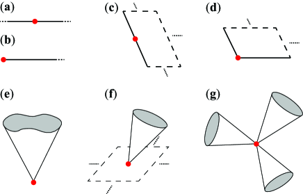
Figure 1: (Color online) Scale-free surfaces and their special points (full circles). All surfaces extend to infinity from their special points as indicated by the dashed lines. Grey areas indicate truncation surfaces for graphical representation, while dashed lines represent similarly truncated surfaces. Dots indicate directions in which the infinite objects are extended. (a) Infinite, and (b) semi-infinite lines in $d=2$ or 3. Semi-infinite (c) half-plane and (d) quarter-plane in $d=3$. (e) Cone with convoluted cross section. Complex shapes created by (f) attaching apex of a cone to a plane, or (g) by joining apices of several cones.

For large $N$ there is a range of distances between $a$ and $R_{e}$ where, in free space, the polymer exhibits self-similar scale-invariant behavior. The presence of boundaries can introduce new length scales. However, there is a group of surfaces, called scale-free (SF), or scale-invariant, such that geometry has no characteristic length scale, i.e., they remain invariant under coordinate transformation $\mathbf{r}\to\lambda\mathbf{r}$, when the origin of coordinates is placed at a special point. Such surfaces as (infinite) circular cones (their apices serve as the special points), or wedges in two and three dimensions, will be discussed in detail in this work. Fig. 1 depicts a variety of such shapes. Complex geometries can be made by joining special points of SF surfaces, as demonstrated in Figs. 1f and g. When an end-point of a polymer is attached to a special point of repulsive SF surface, its exponent $\nu$ is not affected but the prefactor in the relation between $R_{e}$ and $N$ may change. However, SF surface can modify exponent $\gamma$ (see Ref. Maghrebi et al. (2012)). E.g., $\gamma=1/2$ Chandrasekhar (1943) for IP attached to a repulsive plane. For the purposes of this work it is particularly convenient to use the universal exponent $\eta$ which is related to the decay of density correlations. Fisher’s identity Cardy (1996) $\gamma=(2-\eta)\nu$ relates this exponent to the ones mentioned earlier. For IPs in free space $\eta=\eta_{f}=0$, and in the presence of SF surfaces $\eta\geq 0$. The total number of configurations of IPs becomes ${\cal N}\sim b^{N}N^{-\eta/2}$.

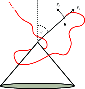
Figure 2: (Color online) Polymer with one end held at position $\mathbf{h}$ from a scale-free surface. The entropic force between the polymer and the surface, which is also the force that acts on the point that holds the end of the polymer has component $F_{\hat{\mathbf{h}}}$ parallel to the vector $\mathbf{h}$, and components $F_{\hat{\mathbf{s}}}$ perpendicular to that direction.

Consider a setup, where one end of a long IP is held at position $\mathbf{h}$ relative to the special point of SF geometry, such as the tip of the cone in Fig. 2). (The vector $\mathbf{h}$ does not have to be along some special symmetry axis.) A significant part of the force exerted by the polymer is coming from distances comparable with $h\equiv|\mathbf{h}|$, while as $N$ grows the tail of the polymer wanders-away from the surface. For $h\ll R_{e}$ the total force that the polymer exerts on the surface, or alternatively the force $\mathbf{F}$ exerted by the surface on the polymer, becomes independent of $R_{e}$. In that limit, the only dimensionally possible form for $\mathbf{F}$ is $k_{B}T/h$, and therefore the component of the total force in the direction of $\hat{\mathbf{h}}=\mathbf{h}/h$ is

$$F_{\hat{\mathbf{h}}}\equiv\mathbf{F}\cdot\hat{\mathbf{h}}=\mathcal{A}\frac{k_{B}T}{h},$$ (1)

where $k_{B}$ is the Boltzmann constant and $T$ is the temperature. It was demonstrated Maghrebi et al. (2011) that the dimensionless amplitude $\mathcal{A}$ in this relation for the radial component of the force is independent of the direction $\hat{\mathbf{h}}$ and only depends on universal exponents, i.e., exponents which do not depend on the microscopic details of the monomers, but depend only on a small number of parameters such as geometry, dimensionality and the presence of self avoiding interaction; for a IP,

$$\mathcal{A}=\eta.$$ (2)

When $\eta_{f}\neq 0$, as in polymers in good solvent, this expression becomes $\mathcal{A}=\eta-\eta_{f}$. In Ref. Maghrebi et al. (2011), $\eta$ was found for IPs in the cases of a cone and a wedge. In this work, we re-derive this law and obtain the value of $\mathcal{A}$ from different considerations, and relate it to the pressure distribution along the boundaries.

In a non-symmetric situation, as depicted in Fig. 2 the force may have additional components in non-radial direction $\hat{\mathbf{s}}\perp\hat{\mathbf{h}}$ which is given by

$$F_{\hat{\mathbf{s}}}\equiv\mathbf{F}\cdot\hat{\mathbf{s}}=\mathcal{A}(\hat{\mathbf{h}},\hat{\mathbf{s}})\frac{k_{B}T}{h},$$ (3)

where the value of this dimensionless amplitude depends both on the direction of the point where the polymer is held and on the direction of the particular force component. We provide a procedure for calculating $\mathcal{A}(\hat{\mathbf{h}},\hat{\mathbf{s}})$, and relate it to the pressure distribution.

In Sec. II we derive a general formalism for calculation of Green and partition functions for SF surfaces, and use it to calculate the force between the polymer and the surface. In Sec. IV we expand the formalism which has been previously used for flat surfaces (Sec. III) to derive general expressions for monomer density and pressure on a SF surface. We also demonstrate a relation between the polymer problem and an electrostatic problem of a point charge located near a conducting surface, and demonstrate various symmetries of the solutions. Specific surface shapes (circular cone in $d=3$, wedge in $d=2$ and $d=3$) are solved in Sec. V. Finally, in Sec. VI we extend our formalism to polymers held at both ends and to ring polymers.

II General formalism for confined ideal polymers

II.1 Ideal polymers confined by arbitrary shapes

IP statistics are closely related to the statistics of random walks (RWs) and diffusion problems Wiegel (1986). An IP with $N+1$ monomers can be modeled as an $N$-step RW. Consider a RW starting from the point $\mathbf{h}$ on a $d$-dimensional hypercubic lattice. The total number of such walks is $\mathcal{N}_{f}(N)=(2d)^{N}$. In the presence of confining boundaries, we denote the total number of walks starting from $\mathbf{h}$ which do not cross the boundaries as $\mathcal{N}_{\text{nc}}(\mathbf{h},N)$, and the number of walks which start at $\mathbf{h}$ and end at $\mathbf{r}$ without crossing the boundaries as $\mathcal{N}_{\text{nc}}(\mathbf{h},\mathbf{r},N)$. In order to investigate the properties of long polymers in confined spaces we focus on the following two functions: the (normalized) partition function (or random walker survival probability),

$$Z(\mathbf{h},N)=\frac{\mathcal{N}_{\text{nc}}(\mathbf{h},N)}{\mathcal{N}_{f}(N)},$$ (4)

and the Green function (or propagator),

$$G(\mathbf{h},\mathbf{r},N)=\frac{\mathcal{N}_{\text{nc}}(\mathbf{h},\mathbf{r},N)}{a^{d}\mathcal{N}_{f}(N)}.$$ (5)

The division by the volume of lattice cell $a^{d}$ converts the probability into probability density in the continuum description. When the relevant distances of the problem are much larger than the lattice constant $a$, both functions can be approximated as continuous functions which obey the diffusion equations Wiegel (1986),

$$\begin{split}&\frac{\partial Z(\mathbf{h},N)}{\partial N}=D\nabla_{\mathbf{h}}^{2}Z(\mathbf{h},N),\\ &Z(\mathbf{h},0)=1,\end{split}$$ (6)

$$\begin{split}&\frac{\partial G(\mathbf{h},\mathbf{r},N)}{\partial N}=D\nabla_{\mathbf{r}}^{2}G(\mathbf{h},\mathbf{r},N)\,\\ &G(\mathbf{h},\mathbf{r},0)=\delta^{d}(\mathbf{h}-\mathbf{r}),\end{split}$$ (7)

where the diffusion constant $D=a^{2}/2d$, while the subscripts $\mathbf{h},\mathbf{r}$ of the Laplacians indicate variables with respect to which the derivatives are taken. In order to exclude all the walks that cross the boundaries, we require that both $Z$ and $G$ vanish on the boundaries. In that respect, a long polymer near a repulsive wall corresponds to diffusion near an absorbing surface.

Since either end of a RW can be considered its beginning or end, the Green function satisfies the reciprocity relation Morse and Feshbach (1953)

$$G(\mathbf{r}_{1},\mathbf{r}_{2},N)=G(\mathbf{r}_{2},\mathbf{r}_{1},N).$$ (8)

The partition and Green functions are related by

$$Z(\mathbf{h},N)=\int G(\mathbf{h},\mathbf{r},N)d^{d}\mathbf{r}.$$ (9)

From $G$ and $Z$ we can calculate the monomer density at a point $\mathbf{r}$ in the allowed space,

$$\rho_{N}(\mathbf{h},\mathbf{r})=\int_{0}^{N}G(\mathbf{h},\mathbf{r},n)Z(\mathbf{r},N-n)dn/Z(\mathbf{h},N).$$ (10)

The expression in the numerator decays with increasing $N$ due to absorbing boundary condition. Since $\int G(\mathbf{h},\mathbf{r},n)Z(\mathbf{r},N-n)d^{d}\mathbf{r}=Z(\mathbf{h},N)$ independently of the value of $n$, the total number of monomers is $\int\rho_{N}(\mathbf{h},\mathbf{r})d^{d}\mathbf{r}=N$. In most of the examples we will consider monomer density for infinite polymers, and therefore the total number of monomers will be infinite. Both $G$ and $Z$ in the integrand of Eq. (10) satisfy diffusion equations with absorbing boundaries, i.e. they both vanish at the boundaries, and approach them with finite slopes. Therefore, the density itself vanishes quadratically close to the boundary.

II.2 Ideal polymers confined by scale-free shapes

In the presence of a scale-free surface, neither Eq. (6) nor the boundary surface introduce any length scale into the problem. Therefore, the partition function depends only on the dimensionless ratio $\mathbf{w}\equiv\mathbf{h}/\sqrt{DN}$, i.e. $Z(\mathbf{h},N)=H(\mathbf{w})$, where $H$ is a dimensionless function. In terms of the reduced variable Eq. (6) becomes Maghrebi et al. (2012)

$$\nabla_{\mathbf{w}}^{2}H+\frac{1}{2}{\bf w}\cdot\vec{\nabla}_{\mathbf{w}}H=0.$$ (11)

When the size of the polymer is significantly larger than $h$, i.e., $w\ll 1$ the second term in the equation becomes negligible, and the equation reduces to

$$\nabla_{\mathbf{w}}^{2}H=0.$$ (12)

In the presence of scale-free surfaces, it is useful to describe the polymer in a coordinate system that separates the radial part from all other coordinates, as is done in spherical or polar coordinates. In many of these systems Moon and Spencer (1971), the Laplace operator can be written in the form

$$\nabla_{\mathbf{w}}^{2}=w^{1-d}\frac{\partial}{\partial w}\left(w^{d-1}\frac{\partial}{\partial w}\right)+w^{-2}\nabla_{S_{d-1}}^{2},$$ (13)

where $\nabla_{S_{d-1}}^{2}$ is the Laplace-Beltrami operator acting on the $d-1$ non-radial coordinates Chavel (1984). Since the boundary conditions on $H$ are independent of $w$, we expect that for $w\ll 1$ the solution can be expressed as a product of a power of $w$ and an angular function $\Theta(\theta_{1},\dots,\theta_{d-1})\equiv\Theta(\hat{\mathbf{w}})$, where $\hat{\mathbf{w}}\equiv\mathbf{w}/w$. In the limit $w\ll 1$ the large-$N$ expression becomes applicable, and it follows that $Z\sim N^{-\eta/2}$. This means that for $w\ll 1$,

$$H(\mathbf{w})\approx w^{\eta}\Theta(\hat{\mathbf{w}})\ \ {\rm or}\ \ Z(\mathbf{h})\approx(h/\sqrt{DN})^{\eta}\Theta(\hat{\mathbf{h}})$$ (14)

By substituting this expression into Eq. (12) and using Eq. (13) we obtain an eigenvalue equation

$$\nabla_{S_{d-1}}^{2}\Theta=\eta(2-d-\eta)\Theta,$$ (15)

that determines $\eta$ and the corresponding eigenfunction $\Theta(\hat{\mathbf{w}})$. This equation has an infinite number of eigenvalues and eigenfunctions, but, since $Z$ (or $H$) is a positive function, we are interested only in the “ground state” solution that is always positive, and corresponds to the lowest value of $\eta$. For example Maghrebi et al. (2012), in the case of a polymer in a wedge of opening angle $2\alpha$ in $d=2$, there is only one angular variable $\theta$ measured, say, from the symmetry axis of the wedge; in this system $\eta=\pi/2\alpha$, while $\Theta(\theta)=\cos(\pi\theta/2\alpha)$. For a $d=3$ circular cone, of apex angle (between the symmetry axis and the surface of the cone) $\alpha$, the value of $\eta$ is determined Maghrebi et al. (2012) by finding the smallest degree $\eta$ of Legendre function satisfying $P_{\eta}(\cos\alpha)=0$. The corresponding $\Theta(\theta,\phi)=P_{\eta}(\cos\theta)$, where $\theta$ is measured from the symmetry axis, and the function is independent of $\phi$ due to symmetry of the problem. For a $d$-dimensional cone, Eq. (15) was solved by Ben-Naim and Krapivsky Ben-Naim and Krapivsky (2010). Their solution was used in Maghrebi et al. (2012, 2011) to find the force amplitude for IPs near cones. Another example for a geometry where Eq. (15) can be solved is a cone with elliptical cross section (see Ref. Boersma and Jansen (1990)).

From Eq. (14) the free energy of the polymer is $\mathcal{F}=-k_{B}T(\eta\ln h+\ln\Theta(\hat{\mathbf{h}}))+{\rm const.}$, from which the force is compiled as

$$F_{\hat{\mathbf{h}}}=-\frac{{\partial\mathcal{F}}}{\partial r}=\eta\frac{k_{B}T}{h},$$ (16)

i.e., the amplitude that was defined in Eq. (1), $\mathcal{A}=\eta$ is independent of the direction of $\hat{\mathbf{h}}$, as stated in Eq. (2). For the amplitude in one of the perpendicular directions $\hat{\mathbf{s}}$, we need to take a similar derivative with respect to coordinate $r_{\hat{\mathbf{s}}}$ perpendicular to $\hat{\mathbf{h}}$.

$$F_{\hat{\mathbf{s}}}=-\frac{{\partial\mathcal{F}}}{\partial r_{\hat{\mathbf{s}}}}=\frac{\Theta^{(\hat{\mathbf{s}})}(\hat{\mathbf{h}})}{\Theta(\hat{\mathbf{h}})}\frac{k_{B}T}{h},$$ (17)

where $\Theta^{(\hat{\mathbf{s}})}$ denotes a (angular) derivative of $\Theta$ on a unit sphere in direction of $\hat{\mathbf{s}}$, such as $\partial/\partial\theta$ in the spherical coordinate system. Thus the amplitude in Eq. (3) is $\mathcal{A}(\hat{\mathbf{h}},\hat{\mathbf{s}})=\Theta^{(\hat{\mathbf{s}})}(\hat{\mathbf{h}})/\Theta(\hat{\mathbf{h}})$.

If the end of a polymer is tethered to the origin by a string of length $h$, but is allowed to fluctuate in non-radial direction, the function $\Theta(\hat{\mathbf{h}})$, that must be normalized, is the probability density for the orientation $\hat{\mathbf{h}}$. Since $\Theta$ is positive in the allowed space (and vanishes only on the boundaries) it will frequently have a single maximum, such as the position of the symmetry axis in the case of a wedge or a cone, although multiple maxima can be created by, say, properly shaping the cross section of a cone. This probability is independent of temperature, and therefore the fluctuations of the end-point will also be temperature independent. In simple geometries the fluctuations will be “large”, i.e., occupy most of the available directions.

The Green function has dimensions [length]^-d and satisfies Eq. (7). It can be written using the same dimensionless variable, $\mathbf{w}$ as well as $\mathbf{v}\equiv\mathbf{r}/\sqrt{DN}$, as

$$G(\mathbf{h},\mathbf{r},N)=(DN)^{-d/2}Y(\mathbf{w},\mathbf{v}),$$ (18)

where $Y$ is a dimensionless function. For $DN\gg h^{2}$ ($w\ll 1$) the system loses its detailed dependence on the initial condition, resulting in a function of $\mathbf{r}$ with $\mathbf{h}$ dependent prefactor. Thus, we attempt a solution of the form

$$\tilde{G}(\mathbf{r},N)=Cg(r,N)\Theta(\hat{\mathbf{r}}),$$ (19)

where unit vector $\hat{\mathbf{r}}\equiv\mathbf{r}/r=\{\theta_{1},\dots\theta_{d-1}\}$ describes the non radial coordinates, and $C$ is a (dimensional) prefactor containing $h,D$. For $g(r,N)$ we use the expression

$$g(r,N)=r^{x}N^{y}\exp\left(-\frac{r^{2}}{4DN}\right).$$ (20)

Note that the exponent $\exp\left(-\frac{r^{2}}{4DN}\right)$ is exactly the same as in the description of an IP in free space. By using Eqs. (13)-(20) in Eq. (7) we get

$$\left[\frac{r^{2}}{DN}\left(\frac{d}{2}+x+y\right)+x(2-d-x)\right]\Theta=\nabla_{S_{d-1}}^{2}\Theta.$$ (21)

In order for Eq. (21) to hold for arbitrary values of $r$, the coefficient of $r$ must vanish, leading to

$$\frac{d}{2}+x+y=0.$$ (22)

The value of $x$ is determined by the eigenvalue equation

$$\nabla_{S_{d-1}}^{2}\Theta=x(2-d-x)\Theta.$$ (23)

This (angular) equation coincides with Eq. (15), but, unlike $H$ in Eq. (12), the function $\tilde{G}$ that we are seeking is not harmonic. Obviously, the value of $x$ in this equation will coincide with $\eta$ that was found in the calculation of $H$, as well as the function $\Theta(\hat{\mathbf{r}})$ will be the same as $\Theta(\hat{\mathbf{w}})$ describing $H$. (We seek the “ground state” value of $x$ since the function $\tilde{G}$ must be positive.) We shall henceforth substitute $\eta$ for $x$. It is shown below that such value of $x$ indeed produces a correct description of the partition function.

Thus we have a solution for the diffusion equation near a scale-free surface. This solution does not satisfy the initial condition in Eq. (7) and does not properly describe the statistics of short polymers, where the size of the polymer approaches $h$. However, $\tilde{G}$ approaches the exact solution for the Green function of long ($\sqrt{DN}\gg h$) IPs near SF surface. Since the form of the Green function must be described by Eq. (18), we must choose the constant in Eq. (19) as $C=ch^{\eta}/D^{\eta+d/2}$, where $c$ is a dimensionless constant (that depends on $\hat{\mathbf{h}}$), leading to

$$\tilde{G}=c\left(\frac{1}{\sqrt{DN}}\right)^{d}\left(\frac{h}{\sqrt{DN}}\right)^{\eta}\left(\frac{r}{\sqrt{DN}}\right)^{\eta}{\rm e}^{-r^{2}/4DN}\Theta(\hat{\mathbf{r}}).$$ (24)

Integration of this expression over the $d$-dimensional space confined by the surfaces, leads (up to a dimensionless prefactor) to the value of $Z(\mathbf{h},N)=H(\mathbf{w})\sim(h/\sqrt{DN})^{\eta}=w^{\eta}$, i.e., the correct behavior of $Z$.

Note that from the definition of $G$ (Eq. (5)) and the boundary conditions, $\Theta$ must be a positive function that vanishes on the boundaries.

When the geometry is complicated, and analytical solution of Eq. (23) cannot be obtained, the force amplitude can be evaluated numerically. This process can be simplified by considering the average position of the polymer end point,

$$R_{e,\tilde{G}}^{2}\equiv\frac{\int r^{2}\tilde{G}(\mathbf{r},N)d^{d}\mathbf{r}}{\int\tilde{G}(\mathbf{r},N)d^{d}\mathbf{r}}=2DN(\eta+d).$$ (25)

[Angular integrals in the numerator and denominator are identical and cancel, while the radial integrals are simple products of powers and Gaussians and lead to this result.] Since $\tilde{G}$ approaches the exact solution in the limit $N\rightarrow\infty$ we can write a formula for the force amplitude,

$$\eta=\lim_{N\rightarrow\infty}\frac{R_{e}^{2}}{2DN}-d.$$ (26)

Note that in free space $\eta=0$, and we recover the usual mean squared end-to-end distance for an IP/random walk $R_{e}^{2}=a^{2}N$. When we confine the polymer by holding it near the boundary the mean squared end-to-end distance grows but it is still linearly proportional to the number of monomers. Using Eq. (26), the force amplitude can be evaluated from numerical solution of the diffusion equation or from simulations of random walks in confined spaces.

III Ideal polymer near a plane

The problem of an IP near a repulsive plane was considered in Refs. Bickel et al. (2001); Breidenich et al. (2007); Jensen et al. (2013). In this section we expand the approach used in Bickel et al. (2001) to general $d$ and set the stage for the treatment of more complicated surfaces.

In $d$ dimensions positions in half-space space are described by $\mathbf{r}=(r_{1},...,r_{d})\equiv(\mathbf{R},r_{\perp})$) with $r_{\perp}>0$. For an IP with one end fixed at $\mathbf{h}=(0,\dots,0,h)$, the Green function can be found using the method of images Chandrasekhar (1943):

$$\begin{split}G(\mathbf{h},\mathbf{r},N)=\left(\frac{1}{4\pi DN}\right)^{d/2}\exp\left(-\frac{R^{2}}{4DN}\right)\times\\ \left\{\exp\left(-\frac{(r_{\perp}-h)^{2}}{4DN}\right)-\exp\left(-\frac{(r_{\perp}+h)^{2}}{4DN}\right)\right\}.\end{split}$$ (27)

The corresponding partition function can be found by integrating Eq. (27) over $\mathbf{r}$,

$$Z(\mathbf{h},N)=\text{erf}\left(h/\sqrt{4\pi DN}\right).$$ (28)

Using Eqs. (10), (27) and (28), and taking the $N\rightarrow\infty$ limit we get for $d>2$,

$$\rho(\mathbf{h},\mathbf{r})=\displaystyle\frac{1}{4D}\frac{\Gamma\left(\frac{d}{2}-1\right)}{\pi^{d/2}}\frac{r_{\perp}}{h}\left\{[R^{2}+(r_{\perp}-h)^{2}]^{1-d/2}\right.$$

$$\left.-[R^{2}+(r_{\perp}+h)^{2}]^{1-d/2}\right\}.$$ (29)

(Henceforth, quantities without index $N$ will denote infinite polymer limit.) For $d=2$,

$$\rho(\mathbf{h},\mathbf{r})=\frac{1}{4\pi D}\frac{r_{\perp}}{h}\ln\frac{R^{2}+(h+r_{\perp})^{2}}{R^{2}+(h-r_{\perp})^{2}}.$$ (30)

When a planar surface is distorted by infinitesimal amount $\Delta(\mathbf{R})$ by shifting it from $r_{\perp}=0$ to $r_{\perp}=\Delta(\mathbf{R})$), the resulting change in the number of available conformations modifies the free energy of the polymer by an amount

$$\Delta\mathcal{F}_{N}=\int\limits_{r_{\perp}=0}\left[P_{N}(\mathbf{R})\Delta(\mathbf{R})\right]d^{d-1}\mathbf{R}+O(\Delta(\mathbf{R})^{2}),$$ (31)

where $P_{N}(\mathbf{R})$ is the entropic pressure of the polymer on the surface at position $\mathbf{R}$. Thus, the pressure represents a variational derivative of the free energy, and for a polymer with one end held at $\mathbf{h}$ it can be written in terms of the Green function Bickel et al. (2001) as

$$P_{N}(\mathbf{h},\mathbf{R})=\frac{k_{B}TD}{Z(\mathbf{h},N)}\int_{0}^{N}\frac{\partial G(\mathbf{r},\mathbf{h},n)}{\partial r_{\perp}}\frac{\partial Z(\mathbf{r},N-n)}{\partial r_{\perp}}dn,$$ (32)

where $\mathbf{r}=(\mathbf{R},r_{\perp})$, and the derivatives are evaluated at $r_{\perp}=0$. Equation (10) can be used to rewrite this expression via the monomer density $\rho(\mathbf{r})$ ,

$$P_{N}(\mathbf{h},\mathbf{R})=\frac{Dk_{B}T}{2}\frac{\partial^{2}}{\partial r_{\perp}^{2}}\rho_{N}(\mathbf{h},\mathbf{r}).$$ (33)

From Eqs. (III), (33) we find the polymer pressure on the plane in the limit $N\rightarrow\infty$,

$$P(R)=\frac{\Gamma(d/2)}{\pi^{d/2}}\frac{k_{B}T}{(R^{2}+h^{2})^{d/2}}.$$ (34)

It should be noted that the infinite-$N$ expressions for the density and the pressure apply to finite-$N$ situations when $DN\gg r^{2},h^{2}$. For smaller $N$ these quantities cannot be expressed in such simple terms. If a polymer is confined to a finite volume and both its ends are free to move, a different approach needs to be used to calculate the pressure distribution (see, e.g., Ref. Grosberg (1972)).

IV Ideal Polymers near General Scale-Free Surfaces

Equation (10) provides a general expression for calculation of monomer density of IP for arbitrary confining surfaces. Usually, such $\rho_{N}$ will be a very complicated function. We will demonstrate that for scale-free surfaces for sufficiently large $N$ the expressions for density (and also for pressure) approach an $N$-independent form that is significantly simpler than the small-$N$ expressions.

IV.1 Monomer Density for Infinite Polymers

Calculation of monomer density $\rho_{N}(\mathbf{h},\mathbf{r})$ in Eq. (10) requires integration of the product $G(\mathbf{h},\mathbf{r},n)Z(\mathbf{r},N-n)$ over $n$ varying from 0 to $N$. In free space the Green function $G(\mathbf{h},\mathbf{r},n)$ is very small for $n$ such that $\sqrt{Dn}\ll|\mathbf{h}-\mathbf{r}|$), because random walk from $\mathbf{h}$ is “too short” to reach $\mathbf{r}$. Similarly, for $\sqrt{Dn}\gg|\mathbf{h}-\mathbf{r}|$ the walk is “too long” to be at $\mathbf{r}$ with a significant probability. Thus, $G$ in free space peaks when $\sqrt{Dn}$ is of order of $|\mathbf{h}-\mathbf{r}|$. In the presence of absorbing boundaries, the large $n$ decay is even stronger. In the presence of scale-free surfaces, for long polymers ($DN\gg h^{2},r^{2}$) it is possible to divide the integral $\int_{0}^{N}$ in Eq. (10) into $\int_{0}^{n_{1}}+\int_{n_{1}}^{N}$, where $r^{2},h^{2}\ll Dn_{1}\ll DN$, and show that for fixed $x_{1}=n_{1}/N$, in the limit $N\to\infty$ the second integral divided by $Z(\mathbf{h},N)$ vanishes. This feature is quantitatively demonstrated in Appendix B. Thus, only the first integral includes significant contributions to the density. In its range ($n<n_{1}\ll N$) we can assume $Z(\mathbf{r},N-n)\approx Z(\mathbf{r},N)$ and take it out of the integration so that in the infinite-$N$ limit the density is $\rho(\mathbf{h},\mathbf{r})=\lim_{N\rightarrow\infty}\left[Z(\mathbf{r},N)/Z(\mathbf{h},N)\right]\int_{0}^{\infty}G(\mathbf{h},\mathbf{r},n)dn$, or using Eq. (14),

$$\rho(\mathbf{h},\mathbf{r})=\frac{\Theta(\hat{\mathbf{r}})}{\Theta(\hat{\mathbf{h}})}\left(\frac{r}{h}\right)^{\eta}\int_{0}^{\infty}G(\mathbf{h},\mathbf{r},n)dn.$$ (35)

This simplification enables us to perform the integral and derive analytical expressions for the monomer density.

Since the density $\rho$ in Eq. (35) depends only on the integral of $G$ it is convenient to define

$$\Phi(\mathbf{h},\mathbf{r})\equiv\int_{0}^{\infty}G(\mathbf{h},\mathbf{r},n)dn.$$ (36)

From Eq. (7),

$$\nabla_{\mathbf{r}}^{2}\Phi(\mathbf{h},\mathbf{r}) = \int_{0}^{\infty}\nabla_{\mathbf{r}}^{2}G(\mathbf{h},\mathbf{r},n)dn$$ (37)

$$= (1/D)(G(\mathbf{h},\mathbf{r},\infty)-G(\mathbf{h},\mathbf{r},0))$$

$$= -(1/D)\delta^{d}(\mathbf{h}-\mathbf{r}),$$

i.e., the density at $\mathbf{r}$ is related to the potential of a point charge at $\mathbf{h}$

$$\rho(\mathbf{h},\mathbf{r})=\frac{\Theta(\hat{\mathbf{r}})}{\Theta(\hat{\mathbf{h}})}\left(\frac{r}{h}\right)^{\eta}\Phi(\mathbf{h},\mathbf{r}).$$ (38)

IV.2 Some properties of monomer density and pressure

The expression for calculation of monomer density of an infinite IP in Eq. (35), requires knowledge of the exact Green function or electrostatic potential. These are frequently expressed as an infinite sum of functions. Since the density $\rho(\mathbf{h},\mathbf{r})$ is singular for $\mathbf{h}=\mathbf{r}$ such expansions of density do not always converge. Even the simple expression for pressure on flat surfaces in Eq. (33) can be expanded in powers of $r/h$, but will converge only for $r<h$. Alternatively, it can be expanded in the powers of $h/r$, and will converge only for $h<r$. This situation will recur for more complicated surfaces discussed in the following section.

If the expression for monomer density in an infinite polymer (35) is combined with the reciprocity relation of the Green function in Eq. (8), or Eq. (38) is combined with the reciprocity property of electrostatic potential, we can relate the monomer densities in the situation when the polymer starting point $\mathbf{r}_{1}$ and the observation point $\mathbf{r}_{2}$ interchange their roles

$$\rho(\mathbf{r}_{1},\mathbf{r}_{2})=\left[\frac{\Theta(\hat{\mathbf{r}}_{2})}{\Theta(\hat{\mathbf{r}}_{1})}\right]^{2}\left(\frac{r_{2}}{r_{1}}\right)^{2\eta}\rho(\mathbf{r}_{2},\mathbf{r}_{1}).$$ (39)

From Eq. (18) it follows that in scale-free geometries $G(\lambda\mathbf{r}_{1},\lambda\mathbf{r}_{2},\lambda^{2}n)=\lambda^{-d}G(\mathbf{r}_{1},\mathbf{r}_{2},n)$, which can be used with Eq. (35) to obtain

$$\rho(\lambda\mathbf{r}_{1},\lambda\mathbf{r}_{2})=\lambda^{2-d}\rho(\mathbf{r}_{1},\mathbf{r}_{2}).$$ (40)

(This relation can also be obtained from the properties of $\Phi$ under rescaling.) This means that the structure of the density function can be slightly simplified: If instead of variables $\mathbf{r}_{1}$ and $\mathbf{r}_{2}$ we use the direction of the two vectors and their lengths $r_{1}$ and $r_{2}$, when the ratio of the lengths is $x=r_{2}/r_{1}$, then by choosing $\lambda=1/r_{1}$ in Eq. (40) we find that $\rho(\mathbf{r}_{1},\mathbf{r}_{2})=r_{1}^{2-d}f(x,\hat{\mathbf{r}}_{1},\hat{\mathbf{r}}_{2})$. We therefore expect that the calculation of density function will involve an expansion of the solution in the dimensionless ratio $x$.

Let us now consider a Kelvin transform of coordinates where the new position is obtained by inverting the old position with respect to a sphere of radius $h$: $\mathbf{r}_{2}=(h/r_{1})^{2}\mathbf{r}_{1}$ (Under this transformation $\mathbf{h}$ maps into itself.) If the potential $\Phi_{1}(\mathbf{h},\mathbf{r}_{1})$ of the original problem is known, then Doob (2001) $\Phi_{2}(\mathbf{h},\mathbf{r}_{2})\equiv(r_{1}/h)^{d-2}\Phi_{1}(\mathbf{h},\mathbf{r}_{1})$ also solves Eq. (37). Usually, performing Kelvin transform requires similar transformation of the boundary surfaces, but in this case the boundary conditions are independent of the length $r_{1}$ and therefore are automatically satisfied for $r_{2}$. This relation together with Eq. (38) leads to the conclusion that

$$\rho(\mathbf{h},\mathbf{r}_{2})=(r_{1}/h)^{d-2-2\eta}\rho(\mathbf{h},\mathbf{r}_{1}).$$ (41)

This feature conveniently connects the values of the density for, say, $r_{1}/h=y<1$ with the values of density at $r_{2}/h=1/y>1$, i.e., the density for $r>h$ can be reconstructed from the density at $r<h$. For $r_{1}\ll h$ the electrostatic potential $\Phi\sim\Theta(\hat{\mathbf{r}}_{1})r_{1}^{\eta}/Dh^{d-2}$, since in that region it satisfies the same equation as $Z$. Therefore, from Eq. (38) we find in that limit $\rho(\mathbf{h},\mathbf{r}_{1})\approx A[\Theta(\hat{\mathbf{r}}_{1})]^{2}r_{1}^{\eta}/Dh^{d-2+2\eta}$, where $A$ is a dimensionless constant. By using Eq. (41) we can now determine that for $r_{2}=h^{2}/r_{1}\gg h$ the density is $\rho(\mathbf{h},\mathbf{r}_{2})\approx A[\Theta(\hat{\mathbf{r}}_{2})]^{2}/Dr_{2}^{d-2}$ with the same coefficient $A$. The latter relation does not depend on $h$, as could be expected in that region. Since $G$ is a solution of diffusion equation, the expression must include the prefactor $1/D$ of dimension [length]^-2. (The same conclusion follows for Eqs. (37) and (38).) Therefore, aside from angular term, the result is the only dimensionally possible expression for the density.

The method presented in Sec. III to compute the entropic pressure of the polymer in half-space can be generalized to any regular surface (i.e., any surface that appears flat when observed from an infinitesimal distance). For a general surface, we define the distortion $\Delta(\tilde{\mathbf{r}})$ to be in the direction perpendicular to the surface, where $\tilde{\mathbf{r}}$ is a point on the surface. The derivative with respect to $r_{\perp}$ in Eqs. (34) now represents derivative in the direction locally perpendicular to the surface.

Pressure on the boundary corresponds to the second derivative with respect to coordinate perpendicular to the boundary. If $\mathbf{r}_{2}$ and $\mathbf{r}_{1}$ are related by Kelvin transform, as mentioned above, and are on the boundary of the surface, then from Eq. (41) it follows that pressures at corresponding points are related by

$$P(\mathbf{h},\mathbf{r}_{2})=(r_{1}/h)^{d+2-2\eta}P(\mathbf{h},\mathbf{r}_{1}).$$ (42)

From these relations, by repeating the argument analogous to the one in the previous paragraph, or directly from the expressions of $\rho$ at very large and very small distances, we can establish that for $r_{2}\gg h$ the expression for pressure has the $h$-independent dimensionally correct form $P(\mathbf{h},\mathbf{r}_{2})\approx B[\Theta^{(\hat{\mathbf{s}})}(\hat{\mathbf{r}}_{2})]^{2}k_{B}T/r_{2}^{d}$, where $\Theta^{(\hat{\mathbf{s}})}(\hat{\mathbf{r}}_{2})$ is the derivative of $\Theta$ on the unit sphere in direction $\hat{\mathbf{s}}$ perpendicular to the boundary, evaluated on the boundary, and $B$ is some dimensionless constant. Using the arguments outlined above we conclude that at short distances $r_{1}\ll h$, the pressure becomes

$$P(\mathbf{h},\mathbf{r}_{1})\approx B[\Theta^{(\hat{\mathbf{s}})}(\hat{\mathbf{r}}_{1})]^{2}k_{B}Tr_{1}^{2(\eta-1)}/h^{d+2(\eta-1)},$$ (43)

with the same $B$.

IV.3 Pressure and the total force

From Eqs. (33) and (38) the expression for the pressure at a point on a surface can be written as

$$P(\mathbf{h},\mathbf{r}) = \frac{Dk_{B}T}{2}\frac{\partial^{2}}{\partial r_{\perp}^{2}}\left[\frac{\Theta(\hat{\mathbf{r}})}{\Theta(\hat{\mathbf{h}})}\left(\frac{r}{h}\right)^{\eta}\Phi(\mathbf{h},\mathbf{r})\right]$$ (44)

$$= Dk_{B}T\nabla_{\mathbf{r}}\left[\frac{\Theta(\hat{\mathbf{r}})}{\Theta(\hat{\mathbf{h}})}\left(\frac{r}{h}\right)^{\eta}\right]\cdot\nabla_{\mathbf{r}}\Phi(\mathbf{h},\mathbf{r}),$$

where we used the fact that both functions vanish on the boundary and their gradients are parallel to each other and perpendicular to the boundaries. This expression can be used to calculate the total force acting in the direction of $\hat{\mathbf{h}}$ by integrating the projection of the force on the desired direction on the entire surface,

$$F_{\hat{\mathbf{h}}} =\int_{S}d\mathbf{S}\cdot\hat{\mathbf{h}}P(\mathbf{h},\mathbf{r})$$

$$= \!\!Dk_{B}T\!\!\int\nabla_{\mathbf{r}}\!\!\cdot\!\!\left\{\hat{\mathbf{h}}\nabla_{\mathbf{r}}\left[\frac{\Theta(\hat{\mathbf{r}})}{\Theta(\hat{\mathbf{h}})}\left(\frac{r}{h}\right)^{\eta}\right]\!\!\cdot\!\!\nabla_{\mathbf{r}}\Phi(\mathbf{h},\mathbf{r})\right\}d^{d}\mathbf{r}.$$

By applying the divergence operator and using the fact that the function in the first square brackets is harmonic while the electrostatic potential satisfies Eq. (37) we find that,

$$F_{\hat{\mathbf{h}}} = Dk_{B}T\int\hat{\mathbf{h}}\cdot\nabla_{\mathbf{r}}\left[\frac{\Theta(\hat{\mathbf{r}})}{\Theta(\hat{\mathbf{h}})}\left(\frac{r}{h}\right)^{\eta}\right](1/D)\delta^{d}(\mathbf{h}-\mathbf{r})d^{d}\mathbf{r}$$ (46)

$$= k_{B}T\int\frac{\partial}{\partial r}\left[\frac{\Theta(\hat{\mathbf{r}})}{\Theta(\hat{\mathbf{h}})}\left(\frac{r}{h}\right)^{\eta}\right]\delta^{d}(\mathbf{h}-\mathbf{r})d^{d}\mathbf{r}$$

$$= \eta k_{B}T/h\ ,$$

which coincides with the general expression for the force in Eq. (1) with $\mathcal{A}=\eta$, as was seen directly in Eq. (16).

Similar calculations can be performed for the force components in an arbitrary direction. If we choose some direction $\hat{\mathbf{s}}\perp\hat{\mathbf{h}}$, we can repeat the above calculation with the new projection direction $\hat{\mathbf{s}}$. Now on the first line of Eq. (46) we will have the product $\hat{\mathbf{h}}\cdot\nabla_{\mathbf{r}}$ replaced by $\hat{\mathbf{s}}\cdot\nabla_{\mathbf{r}}$, which will result in the derivative acting only on $\Theta(\hat{\mathbf{r}})$ in direction $\hat{\mathbf{s}}$ (such as $(1/r)(\partial/\partial\theta)$ in three-dimensional spherical coordinates) leading to exactly the same result as in Eq. (17).

V Specific Geometries

We will now discuss the monomer density and the entropic pressure of an IP on a wedge in $d=2$ and $3$ a cone in $d=3$. The Green functions for the cone and wedge geometries can be found in Appendix A. The calculation was performed according to the procedure described in section IV. For simplicity throughout this section we consider cases where the end of the polymer is held along the symmetry axis of the cone or wedge.

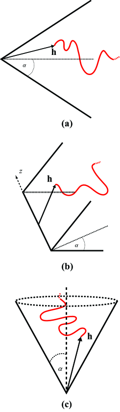
Figure 3: (Color online) An ideal polymer confined to scale-free spaces: (a) wedge in $d=2$, (b) wedge in $d=3$, and (c) circular cone in $d=3$.

V.1 Wedge in $d=2$

Consider a wedge defined in polar coordinates by $-\alpha<\theta<\alpha$ (Fig. 3a). One end of an IP is held at a distance $h$ from the corner, along the symmetry axis of the wedge. The Green function for this geometry is given in Appendix A (Eq. (60)). In the range where $h^{2}\ll DN$ and $r^{2}\lesssim DN$, the sum in Eq. (60) becomes a power series and the lowest power dominates. Thus the Green function converges to the general form presented in Eq. (24). The force amplitude is the lowest power in the series (61), i.e.,

$$\eta=\pi/2\alpha.$$ (47)

In order to derive the monomer density in the wedge, we follow the procedure outlined in section IV. For $N\rightarrow\infty$ we get

$$\begin{split}\rho(\mathbf{r})=\frac{1}{2\pi D}\cos\left(\frac{\pi\theta}{2\alpha}\right)\left(\frac{r}{h}\right)^{\pi/2\alpha}\times\\ \tanh^{-1}\frac{2\cos(\pi\theta/2\alpha)}{(h/r)^{\pi/2\alpha}+(r/h)^{\pi/2\alpha}}\;.\end{split}$$ (48)

The monomer density in a wedge with $\alpha=\pi/3$ is depicted in Fig. 4. The derivative perpendicular to the surface in this geometry is $\frac{\partial}{\partial r_{\perp}}=\frac{1}{r}\frac{\partial}{\partial\theta}$. Using Eqs. (33) and (48) we find the entropic pressure on the surface of the wedge (still for $N\rightarrow\infty$),

$$P(r)=\frac{\pi}{4\alpha^{2}}\frac{k_{B}T}{r^{2}}\frac{1}{1+(h/r)^{\pi/\alpha}}\;.$$ (49)

It is interesting to note the asymptotic behavior of the pressure for small $r$,

$$\lim_{r\rightarrow 0}P(r)\propto r^{\pi/\alpha-2}\rightarrow\begin{cases}0&0<\alpha<\pi/2\\ \mathrm{const.}&\alpha=\pi/2\\ \infty&\pi/2<\alpha<\pi\end{cases}.$$ (50)

When the polymer is held outside the wedge ($\alpha>\pi/2$) the pressure on the tip diverges. This behavior can be seen In Fig. 5, where we plot the pressure on the wedge for three different opening angles. The singularity at the tip of the wedge is similar (but not identical) to the one found in the electric field near the tip of a charged conductor. The analogy to electric fields is not surprising, since we have seen that the monomer density is related to the electrostatic potential of a point charge (Eq. (38)). The electric field near the tip of a conducting wedge scales as $r^{\pi/2\alpha-1}$ Jackson (1998), whereas the polymer pressure scales as $r^{\pi/\alpha-2}$ (see Eq. (50)). For a flat plane ($\alpha=\pi/2$), both powers vanish.

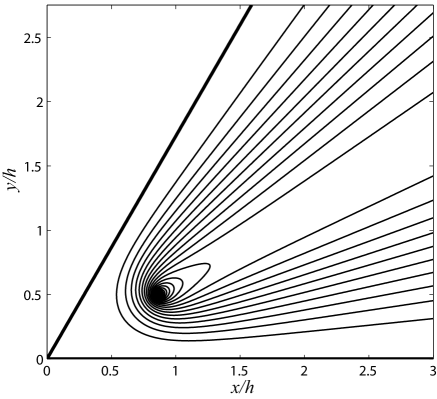
Figure 4: Contour plot of the monomer density for a long ideal polymer with one end held at a distance $h$ from the tip of a wedge ($d=2$) with opening angle $2\alpha=\pi/3$. The boundary is marked by the thick solid line. The density is highest at the origin of the polymer, and the constant density lines are equally separated on a linear scale.

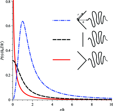
Figure 5: (Color online) Scaled entropic pressure of a long ideal polymer on a wedge ($d=2$) as a function of the scaled distance from the tip for three opening angles of the wedge, $\alpha=\pi/4$ (dot-dashed line), $\alpha=\pi$ (dashed line), $\alpha=3\pi/4$ (solid line).

V.2 Wedge in $d=3$

The boundary of a wedge in 3-dimensional space is defined in cylindrical coordinates by $-\alpha<\theta<\alpha$ (Fig. 3b). Consider a case where one end of the polymer is held at a distance $h$ from the corner, along the symmetry axis of the wedge, at $z=0$. The Green function for this geometry is given in Eq. (63). It is obtained by multiplying the Green function of the wedge in $d=2$ by the $d=1$ free space propagator. When $z^{2}\ll DN$, the Green function is independent of $z$ and when in addition $h^{2}\ll DN$, $r^{2}\lesssim DN$, it assumes the general form of Eq. (24). The force amplitude is the one found in $d=2$ (Eq. (47)). The monomer density in the wedge in the limit $N\rightarrow\infty$ is

$$\rho(r,\theta,z)=\frac{1}{\pi^{1/2}D\alpha}\frac{\left(r/h\right)^{\pi/2\alpha}}{(r^{2}+h^{2}+z^{2})^{1/2}}\cos\left(\frac{\pi\theta}{2\alpha}\right)\times\\ \sum_{i=1}^{\infty}\Gamma\left(\frac{1}{2}+\frac{\pi i}{2\alpha}\right)\sin\left(\frac{\pi i}{2}\right)\cos\left(\frac{i\pi\theta}{2\alpha}\right)\times\\ \left(\frac{rh}{r^{2}+h^{2}+z^{2}}\right)^{i\pi/2\alpha}\times\\ {}_{2}\tilde{F}_{1}\left[\frac{1}{4}+\frac{i\pi}{4\alpha},\frac{3}{4}+\frac{i\pi}{4\alpha},1+\frac{i\pi}{2\alpha},\left(\frac{2rh}{r^{2}+h^{2}+z^{2}}\right)^{2}\right],$$ (51)

where ${}_{2}\tilde{F}_{1}$ is the regularized hypergeometric function. The pressure on the surface of the wedge is

$$P(r,z)=\frac{k_{B}T\pi^{3/2}}{8\alpha^{3}}\frac{(r/h)^{\pi/2\alpha}}{r^{2}(r^{2}+h^{2}+z^{2})^{1/2}}\times\\ \sum_{i=1}^{\infty}i\sin\left(\frac{\pi i}{2}\right)\left(\frac{rh}{r^{2}+h^{2}+z^{2}}\right)^{\pi i/2\alpha}\Gamma\left(\frac{1}{2}+\frac{i\pi}{2\alpha}\right)\times\\ {}_{2}\tilde{F}_{1}\left[\frac{1}{4}+\frac{i\pi}{4\alpha},\frac{3}{4}+\frac{i\pi}{4\alpha},1+\frac{i\pi}{2\alpha},\left(\frac{2rh}{r^{2}+h^{2}+z^{2}}\right)^{2}\right].$$ (52)

Note that at the tip of the wedge we get the same irregular behavior that was encountered for $d=2$, i.e. for $r\ll h$,

$$\underset{r\rightarrow 0}{\lim}P\propto\frac{r^{\pi/\alpha-2}}{(h^{2}+z^{2})^{(\pi/\alpha+1)/2}}.$$

The unusual influence of the geometry of two- and three-dimensional wedges is known in the theory or critical phenomena and the remarkable effects of such geometries have been studied in detail Hanke et al. (1999a) in the context of critical adsorption of liquids.

V.3 Circular Cone in $d=3$

Now consider a cone defined in spherical coordinates by $\theta<\alpha$ (Fig. 3c). The polymer is confined to the cone with one end held at a distance $h$ from the tip along the symmetry axis of the cone. The Green function for this geometry is given in Appendix A. Once more, it contains a sum which becomes a power series when $h^{2}\ll DN$, $r^{2}\lesssim DN$. As in the case of the wedge, in the limit $N\rightarrow\infty$ the first term in the series is dominant, and the Green function converges to the general form of Eq. (24). The force amplitude, $\eta$, is the lowest root of the equation

$$P_{\eta}(\cos\alpha)=0,$$ (53)

where $P_{\eta}$ is the Legendre function. When we apply the procedure described above to calculate the monomer density in the limit $N\rightarrow\infty$, we find

$$\begin{split}&\rho(\mathbf{r})=-\frac{1}{2\pi D\sqrt{hr}}P_{\eta}(\mu)\left(\frac{r}{h}\right)^{\eta}\times\\ &\sum_{i=1}^{\infty}\left(\left[(1-\mu_{0}^{2})\frac{\partial}{\partial\mu}P_{\eta_{i}}(\mu_{0})\frac{\partial}{\partial\eta_{i}}P_{\eta_{i}}(\mu_{0})\right]^{-1}\times\right.\\ &\left.P_{\eta_{i}}(\mu)\begin{cases}(r/h)^{\eta_{i}+1/2}&r<h\\ (h/r)^{\eta_{i}+1/2}&r>h\end{cases}\right),\end{split}$$ (54)

where $\eta_{i}$ are the roots of Eq. (53), in ascending order, $\eta=\eta_{1}$, $\mu=\cos\theta$ and $\mu_{0}=\cos\alpha$. The derivative in the direction perpendicular to the surface is the same as in the case of the wedge (with $\theta$ being the polar angle in spherical coordinates). The pressure on the surface is

$$\begin{split}&P(r)=-\frac{k_{B}T}{2\pi r^{3}}\frac{\partial}{\partial\mu}P_{\eta}(\mu_{0})\times\\ &\begin{cases}(\frac{r}{h})^{\eta+1}\sum_{i=1}^{\infty}\frac{(r/h)^{\eta_{i}}}{\frac{\partial}{\partial\eta_{i}}P_{\eta_{i}}(\mu_{0})}&r<h\\ (\frac{r}{h})^{\eta}\sum_{i=1}^{\infty}\frac{(h/r)^{\eta_{i}}}{\frac{\partial}{\partial\eta_{i}}P_{\eta_{i}}(\mu_{0})}&r>h\end{cases}\end{split},$$ (55)

Note that for $r\rightarrow 0$ we get $P\propto r^{2(\eta-1)}$. The singular asymptotic behavior of the pressure on the tip of the cone is similar to the one found on the wedge (Eq. (50)). It is also similar to the behavior of electric fields near the tip of a conducting cone, where the field scales as $r^{\eta-1}$. For a flat plane ($\alpha=\pi/2$, $\eta=1$), the powers vanish. In fact, if we consider a point charge $q$ held at height $h$ above a grounded conducting plane, the electric field on the plane is identical with the polymer pressure on a flat plane if we replace $k_{B}T/2\pi$ by $2qh$.

VI Polymers Held at both Ends
and Ring Polymers

Consider an IP held at both ends at points $\mathbf{h}_{1}$ and $\mathbf{h}_{2}$ close to scale-free surface as depicted in Fig. 6. The monomer density at a point $\mathbf{r}$ in the allowed space is

$$\rho_{N}(\mathbf{h}_{1},\mathbf{h}_{2},\mathbf{r})=\frac{\int_{0}^{N}G(\mathbf{h}_{1},\mathbf{r},n)G(\mathbf{r},\mathbf{h}_{2},N-n)dn}{G(\mathbf{h}_{1},\mathbf{h}_{2},N)}.$$ (56)

For large $N$, such that $h_{1}^{2},h_{2}^{2}\ll DN$, we can follow the same reasoning as in the subsection IV.1, and divide the integral $\int_{0}^{N}$ into three parts $\int_{0}^{n_{1}}+\int_{n_{1}}^{N-n_{1}}+\int_{N-n_{1}}^{N}$, where $n_{1}$ was chosen such that $h_{1}^{2},h_{2}^{2}\ll Dn_{1}\ll DN$. (Note, that when the integration variable $n$ is replaced by $N-n$ in the third integral, it becomes similar to the first integral with the roles of $\mathbf{h}_{1}$ and $\mathbf{h}_{2}$ reversed.) The first Green function in the integrand of Eq. (56) provides a significant contribution to the integral $\int_{0}^{n_{1}}$, while the second Green function is similarly significant in $\int_{N-n_{1}}^{N}$. Both functions are negligible in $\int_{n_{1}}^{N-n_{1}}$. In fact it can be shown that for fixed $x_{1}=n_{1}/N$, in the $N\to\infty$ limit, the latter integral divided by $G(\mathbf{h}_{1},\mathbf{h}_{2},N)$ vanishes. In the range of the first integral ($n<n_{1}\ll N$) we can assume $G(\mathbf{r},\mathbf{h}_{2},N-n)\approx G(\mathbf{r},\mathbf{h}_{2},N)$ and take it out of the integration so that for large $N$ the contribution of this integral to the density becomes $\left[G(\mathbf{r},\mathbf{h}_{2},N)/G(\mathbf{h}_{1},\mathbf{h}_{2},N)\right]\int_{0}^{x_{1}N}G(\mathbf{h}_{1},\mathbf{r},n)dn$. For large $N$ the ratio of the Green functions preceding the integral can be replaced by the ratio of $\tilde{G}$ functions defined in Eq. (19), which, by using Eq. (24) and the reciprocity relation (8), becomes $(r/h_{1})^{\eta}[\Theta(\hat{\mathbf{r}})/\Theta(\hat{\mathbf{h}}_{1})]$. Similar treatment, with the roles of $\mathbf{h}_{1}$ and $\mathbf{h}_{2}$ reversed, can be performed for the integral $\int_{(1-x_{1})N}^{N}$. The results discussed above become exact in the $N\to\infty$ limit leading to

$$\rho(\mathbf{h}_{1},\mathbf{h}_{2},\mathbf{r}) = \left(\frac{r}{h_{1}}\right)^{\eta}\frac{\Theta(\hat{\mathbf{r}})}{\Theta(\hat{\mathbf{h}}_{1})}\int\limits_{0}^{\infty}G(\mathbf{h}_{1},\mathbf{r},n)dn$$ (57)

$$+ \left(\frac{r}{h_{2}}\right)^{\eta}\frac{\Theta(\hat{\mathbf{r}})}{\Theta(\hat{\mathbf{h}}_{2})}\int\limits_{0}^{\infty}G(\mathbf{h}_{2},\mathbf{r},n)dn.$$

By comparing this result with Eqs. (57) and (35), we see that the contribution from each end of the chain will be equal to the density calculated before for a polymer with one free end, i.e.,

$$\rho(\mathbf{h}_{1},\mathbf{h}_{2},\mathbf{r})=\rho(\mathbf{h}_{1},\mathbf{r})+\rho(\mathbf{h}_{2},\mathbf{r}),$$ (58)

where $\rho(\mathbf{h}_{i},\mathbf{r})$ is the density which was calculated in sections III-V with $\mathbf{h}=\mathbf{h}_{i}$. This result could be expected since the strands leaving the end-points $\mathbf{h}_{1}$ and $\mathbf{h}_{2}$ do not interact with each other, and the mid-section of the polymer is so far away, that the fact that this is a single polymer rather than two independent strands does not influence the density. From the relation between the monomer density and the pressure on the surface (Eq. (33)) we see that this additive correspondence between a pair of IP strands and a single polymer held by both ends will also apply to the pressure and the total force on the surface. This result can also be immediately applied to the density of infinite ring polymers:

$$\rho_{\text{ring}}(\mathbf{h},\mathbf{r})=\rho(\mathbf{h},\mathbf{h},\mathbf{r})=2\rho(\mathbf{h},\mathbf{r}),$$ (59)

as well as to the pressure exerted by such polymers.

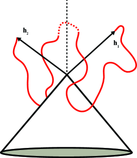
Figure 6: (Color online) Ideal polymer with both ends held near a scale-free surface.

VII Discussion and conclusions

In Ref. Maghrebi et al. (2011) it was shown that the force between a polymer and a scale-free surface can be written in terms of universal exponents, which depend on the geometry of the surface and the nature of the interactions between the monomers, but are independent of the microscopic details of the system. In this paper we have shown that the universal exponent $\eta$ also plays an important role in the monomer density and the pressure of IPs on scale-free surfaces. Additional calculations were needed to completely describe the pressure and the density, but $\eta$ controlled the behavior at very short distances. We found the general form of the Green function $\tilde{G}$ (Eq. (24)) for long IPs. By using the simple connection between the exponent $\eta$ and the mean end-to-end distance of the polymer $R_{e}$ (Eq. (26)), one can measure $\eta$ by solving the diffusion equation numerically or extracting $R_{e}$ from simulations.

In section IV we showed that the monomer density and the entropic pressure can be derived from the electrostatic potential of a point charge in a confined space. It was also shown that the density possesses some powerful scaling properties that enable one to map the density and the pressure from points near the origin to points far away, and vice versa. The relation to electrostatics also enabled the use of a formalism resembling Gauss’ law in electrostatics, to relate the total force to the pressure distribution.

Our calculations were limited to IPs. While they provide some guidance to understanding polymers in good solvents, several important differences exist. The presence of repulsion between monomers modifies both exponent $\nu$ and $\eta$. The basic expression (10) cannot be used in its simplest form to calculate the density because the probability of a polymer reaching point $\mathbf{r}$ in $n$ steps is influenced by the presence of the remaining $N-n$ steps, and proper adjustments need to be made. Even in free space the distribution of the the end-to-end distance of self-avoiding polymers is significantly more complicated (see, Caracciolo et al. (2000) and references therein) than the Green function of ideal polymers. Thus, we cannot expect such simple behaviors as exhibited by $\tilde{G}$ in (24). Nevertheless, we may expect some qualitative similarities between IP and self-avoiding polymers. Polymer adsorption to curved surfaces Eisenriegler et al. (1996) introduces yet another dimension into the problem deserving a detailed study.

In good solvents the density of the monomers no longer decays quadratically with the distance $x$ from the boundary. Scaling analysis shows Joanny et al. (1979) that close to the walls the density scales as $x^{1/\nu}$. (In good solvent $1/\nu<2$ de Gennes (1979).) Bickel et al. Bickel et al. (2001) used this scaling law to compare the behavior of IPs to self-avoiding polymers near flat surfaces, and found numerous qualitative (and even quantitative) parallels between the two cases. It remains to be seen if such parallels can be found in connection with the properties discussed in this paper. Hanke et al. Hanke et al. (1999b) found interesting depletion effects of polymers in good solvent near curved surfaces.

The properties of the monomer density discussed in Sec. VI indicate that the results in this paper can be applied to entropic systems where both ends of the polymer are attached to scale-free surfaces. This may provide a pathway to dealing with polymers attached by both ends to different surfaces, such as a polymer with one end grafted to an AFM tip and the other to a flat substrate. In good solvents expressions like (58) and (59) are obviously incorrect. However, like in IPs, we expect that for very long polymer the behavior of two ends of a polymer will be the same as that of two (interacting) polymers with their remote ends completely free.

Appendix A Green and Partition Functions

Below we list the exact solutions of Eq. (7) that were used to derive the results in this paper. These solutions were taken from Ref. Carslaw and Jaeger (1959).

Wedge in $d=2$: The wedge defined in Fig. 3 is described in polar coordinates by $-\alpha<\theta<\alpha$. The exact solution of Eq. (7) is Carslaw and Jaeger (1959)

$$G(r^{\prime},\theta^{\prime},r,\theta,N)=\frac{1}{2\alpha DN}\exp\left(-\frac{r^{2}+r^{\prime 2}}{4DN}\right)\sum_{i=1}^{\infty}I_{\eta_{i}}\left(\frac{rr^{\prime}}{2DN}\right)\cos(\eta_{i}\theta)\cos(\eta_{i}\theta^{\prime}),$$ (60)

where

$$\eta_{i}=\frac{i\pi}{2\alpha},\;\;i=1,2,3,\dots$$ (61)

and $I_{\eta_{i}}$ is the modified Bessel function of the first kind. The partition function can be found by integrating Eq. (60):

$$Z(r^{\prime},\theta^{\prime},N) = \int G(r^{\prime},\theta^{\prime},r,\theta,N)rdrd\theta$$ (62)

$$= \frac{r^{\prime}}{\sqrt{\pi DN}}\exp\left(-\frac{r^{2}}{8DN}\right)\sum_{i=1}^{\infty}\frac{1}{i}\left[I_{\frac{\eta_{i}-1}{2}}\left(\frac{r^{\prime 2}}{8DN}\right)+I_{\frac{\eta_{i}+1}{2}}\left(\frac{r^{\prime 2}}{8DN}\right)\right]\sin^{2}\left(\frac{\pi i}{2}\right)\cos\left(\eta_{i}\theta^{\prime}\right).$$

Wedge in $d=3$: The solution in $d=3$ is obtained by multiplying the Green function of a wedge in $d=2$ by the free space propagator in $d=1$ leading to

$$G(r^{\prime},\theta^{\prime},z^{\prime},r,\theta,z,N)=\frac{1}{4\alpha\pi^{1/2}(DN)^{3/2}}\exp\left(-\frac{(z-z^{\prime})^{2}}{4DN}\right)\sum_{i=1}^{\infty}\exp\left(-\frac{r^{2}+r^{\prime 2}}{4DN}\right)I_{\eta_{i}}\left(\frac{rr^{\prime}}{2DN}\right)\cos(\eta_{i}\theta^{\prime})\cos(\eta_{i}\theta).$$ (63)

Integrating Eq. (63) one can immediately see that the partition function for the wedge in $d=3$ does not depend on the $z$ coordinate. In fact it is identical with the partition function for the wedge in $d=2$ in Eq. (62).

Circular cone: Circular cone in $d=3$ is defined in spherical coordinates by $\theta<\alpha$ (Fig. 3c). The solution to Eq. (7) in the cone is Carslaw and Jaeger (1959)

$$G(r^{\prime},\theta^{\prime},\phi^{\prime},r,\theta,\phi,N)=-\frac{1}{4\pi DN\sqrt{rr^{\prime}}}\exp\left(-\frac{r^{2}+r^{\prime 2}}{4DN}\right)\sum_{i=1}^{\infty}\left\{I_{\eta_{i}+1/2}\left(\frac{rr^{\prime}}{2DN}\right)(2\eta_{i}+1)\right.\times\\ \sum_{m=0}^{\infty}(2-\delta_{m,0})P_{\eta_{i}}^{-m}(\mu)P_{\eta_{i}}^{-m}(\mu^{\prime})\cos(m(\phi-\phi^{\prime}))\left.\left[(1-\mu_{0})^{2}\frac{\partial}{\partial\mu}P_{\eta_{i}}^{-m}(\mu_{0})\frac{\partial}{\partial\eta}P_{\eta_{i}}^{-m}(\mu_{0})\right]^{-1}\right\},$$ (64)

where $P_{\eta}^{-m}$ are associated Legendre functions, $\mu=\cos\theta$, $\mu_{0}=\cos\alpha$ and ${\eta_{i}}$ are the roots of the equation $P_{\eta}(\mu_{0})=0$ in ascending order. The Green function is somewhat simpler when the starting point of the polymer is along the symmetry axis of the cone, i.e., $\theta^{\prime}=0$. In this case the solution does not depend on the azimuthal angle $\phi^{\prime}$. Denoting $r^{\prime}=h$, we get

$$G(h,r,\theta,N)=-\frac{1}{4\pi DN\sqrt{hr}}\exp\left(-\frac{r^{2}+h^{2}}{4DN}\right)\sum_{i=1}^{\infty}\frac{I_{\eta_{i}+1/2}\left(\frac{rh}{2DN}\right)(2\eta_{i}+1)P_{\eta_{i}}(\mu)}{(1-\mu_{0}^{2})\frac{\partial}{\partial\mu}P_{\eta_{i}}(\mu_{0})\frac{\partial}{\partial\eta}P_{\eta_{i}}(\mu_{0})}.$$ (65)

The partition function can be found for any $\mathbf{r}^{\prime}$ by integrating Eq. (64),

$$Z (r^{\prime},\theta^{\prime},N)=\int r^{2}\sin\theta G(r^{\prime},\theta^{\prime},\phi^{\prime},r,\theta,\phi,N)drd\theta d\phi$$ (66)

$$= e^{-\frac{r^{\prime 2}}{4DN}}\sum_{i=1}^{\infty}\Gamma\left(\frac{3+\eta_{i}}{2}\right){}_{1}\tilde{F}_{1}\left(\frac{3+\eta_{i}}{2},\frac{3}{2}+\eta_{i},\frac{r^{\prime 2}}{4DN}\right)P_{\eta_{i}}(\mu)\left(\frac{r^{\prime 2}}{4DN}\right)^{\eta_{i}/2}\frac{P_{\eta_{i}+1}(\mu_{0})-P_{\eta_{i}-1}(\mu_{0})}{(1-\mu_{0})^{2}\frac{\partial}{\partial\mu}P_{\eta_{i}}(\mu_{0})\frac{\partial}{\partial\eta}P_{\eta_{i}}(\mu_{0})},\$$

where ${}_{1}\tilde{F}_{1}$ is the regularized confluent hypergeometric function Gradshteyn and Ryzhik (2000). Note that due to the cylindrical symmetry $Z$ does not depend on the azimuthal angle $\phi^{\prime}$.

Appendix B Monomer Density in the $N\rightarrow\infty$ limit

In the calculation of the monomer density and the entropic pressure we examined separately the contribution of different parts of the polymer. The monomer density in the limit $N\rightarrow\infty$ is given by

$$\rho(\mathbf{h},\mathbf{r})=\lim_{N\rightarrow\infty}\int\limits_{n=0}^{N}G(\mathbf{h},\mathbf{r},n)Z(\mathbf{r},N-n)dn/Z(\mathbf{h},N).$$ (67)

In order to evaluate this integral we select the ratio $x_{1}=n_{1}/N$ such that $0<x_{1}\ll 1$ and split the integral in Eq. (67),

$$\rho(\mathbf{h},\mathbf{r}) = \lim_{N\rightarrow\infty}\left\{\left(\int\limits_{0}^{n_{1}}+\int\limits_{n_{1}}^{N-n_{1}}+\int\limits_{N-n_{1}}^{N}\right)G(\mathbf{h},\mathbf{r},n)Z(\mathbf{r},N-n)dn/Z(\mathbf{h},N)\right\}$$

$$= \lim_{N\rightarrow\infty}\left\{N\left(\int\limits_{0}^{x_{1}}+\int\limits_{x_{1}}^{1-x_{1}}+\int\limits_{1-x_{1}}^{1}\right)G(\mathbf{h},\mathbf{r},n)Z(\mathbf{r},N-n)dx/Z(\mathbf{h},N)\right\},$$

where we have changed the variable of integration to $x=n/N$. Using the scaling properties of the functions $G$ and $Z$ for large $N$ ($G$ scales as in Eq. (24) and $Z(\mathbf{h},N)=\left(h/\sqrt{DN}\right)^{\eta}\Theta(\hat{\mathbf{h})}$ as in Eq. (14)), we see that in the limit $N\rightarrow\infty$, for $n_{1}<n<N-n_{1}$,

$$G(\mathbf{h},\mathbf{r},n) \propto \left(\frac{1}{N}\right)^{d/2+\eta}G^{*}(\mathbf{h},\mathbf{r},x),$$

$$Z(\mathbf{r},N-n) \propto \left(\frac{1}{N}\right)^{\eta/2}Z^{*}(\mathbf{r},1-x),$$

where $Z^{*}$ and $G^{*}$ do not depend on $N$. Therefore,

$$N\int\limits_{x_{1}}^{1-x_{1}}G(\mathbf{h},\mathbf{r},n)Z(\mathbf{r},N-n)dx/Z(\mathbf{h},N)\propto\left(\frac{1}{N}\right)^{d/2+\eta-1}\rightarrow 0.$$

Since for $x\rightarrow 1$ the partition function $Z(\mathbf{r},N-n)\rightarrow 1$ and becomes independent of $N$, and it is always smaller than one (it is the survival probability of a random walker), in the same limit,

$$N\int\limits_{1-x_{1}}^{1}G(\mathbf{h},\mathbf{r},n)Z(\mathbf{r},N-n)dx/Z(\mathbf{h},N)\propto\left(\frac{1}{N}\right)^{d/2+\eta/2-1}\rightarrow 0.$$

Only the first part of the polymer will contribute to the monomer density in the limit of an infinitely long polymer, as described in the main text, and will lead to density in Eq. (35).

References

- de Gennes (1979) P. G. de Gennes, Scaling Concepts in Polymer Physics (Cornell University Press, 1979).
- Binder (1983) K. Binder, in Phase Transitions and Critical Phenomena, edited by C. Domb and J. L. Lebowitz (Academic Press, London, 1983), vol. 8, pp. 1–144.
- Eisenriegler (1993) E. Eisenriegler, Polymers Near Surfaces: Conformation Properties and Relation to Critical Phenomena (World Scientific, Singapore, 1993).
- Zlatanova and van Holde (2006) J. Zlatanova and K. van Holde, Mol. Cell 24, 317 (2006).
- Leuba and Zlatanova (2001) S. H. Leuba and J. Zlatanova, Biology at the Single Molecule Level (Pergamon, Amsterdam, 2001).
- Binnig et al. (1986) G. Binnig, C. F. Quate, and C. Gerber, Phys. Rev. Lett. 56, 930 (1986).
- Morita et al. (2002) S. Morita, R. Wiesendanger, and E. Meyer, Noncontact Atomic Force Microscopy, vol. 1 (Springer, New York, 2002).
- Sarid (1994) D. Sarid, Scanning Force Microscopy, vol. 5 (Oxford University Press, 1994).
- Bubis et al. (2009) R. Bubis, Y. Kantor, and M. Kardar, Europhys. Lett. 88, 48001 (2009).
- Maghrebi et al. (2011) M. F. Maghrebi, Y. Kantor, and M. Kardar, Europhys. Lett. 96, 66002 (2011).
- Maghrebi et al. (2012) M. F. Maghrebi, Y. Kantor, and M. Kardar, Phys. Rev. E 86, 061801 (2012).
- Evans and Rawicz (1997) E. Evans and W. Rawicz, Phys. Rev. Lett. 79, 2379 (1997).
- Auth and Gompper (2003) T. Auth and G. Gompper, Phys. Rev. E 68, 051801 (2003).
- Guo et al. (2009) K. Guo, J. Wang, F. Qiu, H. Zhang, and Y. Yang, Soft Matter 5, 1646 (2009).
- Laradji (2002) M. Laradji, Europhys. Lett. 60, 594 (2002).
- Nikolov et al. (2007) V. Nikolov, R. Lipowsky, and R. Dimova, Biophys. J. 92, 4356 (2007).
- Werner and Sommer (2010) M. Werner and J. U. Sommer, Eur. Phys. J. E 31, 383 (2010).
- Chandrasekhar (1943) S. Chandrasekhar, Rev. Mod. Phys. 15, 1 (1943).
- Cardy (1996) J. Cardy, Scaling and Renormalization in Statistical Physics, vol. 5 (Cambridge University Press, 1996).
- Wiegel (1986) F. W. Wiegel, Introduction to Path-Integral Methods in Physics and Polymer Science (World Scientific, Singapore, 1986).
- Morse and Feshbach (1953) P. M. Morse and H. Feshbach, Methods of Theoretical Physics, vol. 1 (McGraw-Hill, New York, 1953).
- Moon and Spencer (1971) P. H. Moon and D. E. Spencer, Field Theory Handbook (Springer, Berlin, 1971).
- Chavel (1984) I. Chavel, Eigenvalues in Riemannian Geometry, vol. 115 (Academic press, Waltham, Massachusetts, 1984).
- Ben-Naim and Krapivsky (2010) E. Ben-Naim and P. L. Krapivsky, J. Phys. A 43, 495007 (2010).
- Boersma and Jansen (1990) J. Boersma and J. K. M. Jansen, Electromagnetic Field Singularities at the Tip of an Elliptic Cone (Eindhoven University of Technology, 1990).
- Bickel et al. (2001) T. Bickel, C. Jeppesen, and C. M. Marques, Eur. Phys. J. E 4, 33 (2001).
- Breidenich et al. (2007) M. Breidenich, R. R. Netz, and R. Lipowsky, Europhys. Lett. 49, 431 (2007).
- Jensen et al. (2013) I. Jensen, W. G. Dantas, C. M. Marques, and J. F. Stilck, J. Phys. A 46, 115004 (2013).
- Grosberg (1972) A. Y. Grosberg, Proc. Moscow State Univ., Physics Series 1, 14 (1972).
- Doob (2001) J. L. Doob, Classical Potential Theory and its Probabilistic Counterpart, vol. 262 (Springer, Berlin, 2001).
- Jackson (1998) J. D. Jackson, Classical Electrodynamics (Wiley, Hoboken, New Jersey, 1998), 3rd ed.
- Hanke et al. (1999a) A. Hanke, M. Krech, F. Schlesener, and S. Dietrich, Phys. Rev. E 60, 5163 (1999a).
- Caracciolo et al. (2000) S. Caracciolo, M. S. Causo, and A. Pelissetto, J. Chem. Phys. 112, 7693 (2000).
- Eisenriegler et al. (1996) E. Eisenriegler, A. Hanke, and S. Dietrich, Phys. Rev. E 54, 1134 (1996).
- Joanny et al. (1979) J. F. Joanny, L. Leibler, and P. G. de Gennes, J. Polym. Sci. Polym. Phys. Ed. 17, 1073 (1979).
- Hanke et al. (1999b) A. Hanke, E. Eisenriegler, and S. Dietrich, Phys. Rev. E 59, 6853 (1999b).
- Carslaw and Jaeger (1959) H. S. Carslaw and J. C. Jaeger, Conduction of Heat in Solids, vol. 1 (Oxford University Press, 2nd ed., 1959).
- Gradshteyn and Ryzhik (2000) I. S. Gradshteyn and I. M. Ryzhik, Table of Integrals, Series and Products (Academic Press, London, 2000).