The Teichmüller and Riemann Moduli Stacks

Abstract.

The aim of this paper is to study the structure of the Teichmüller and Riemann moduli spaces, viewed as stacks over the category of complex analytic spaces, for higher-dimensional manifolds. We show that both stacks are analytic in the sense that they admit a smooth analytic groupoid as atlas. We then show how to construct explicitly such an atlas as a sort of generalized holonomy groupoid for such a structure. This is achieved under the sole condition that the dimension of the automorphism group of each structure is bounded by a fixed integer. All this can be seen as an answer to Question 1.8 of [40].

1. Introduction.

Let $X$ be a smooth oriented compact surface. The Teichmüller space $\mathcal{T}(X)$ is defined as the quotient space of the set of smooth integrable complex operators compatible with the orientation (o.c.)

$$\mathcal{I}=\{J\ :\ TX\longrightarrow TX\mid J^{2}\equiv-Id,\ J\text{ o.c.}\}$$

by $\text{Diff}^{0}(X)$, the connected component of the identity in the oriented diffeomorphism group $\text{Diff}^{+}(X)$ of $X$.

The theory of Teichmüller spaces is a cornerstone in complex variables and Riemann surfaces. Originated by Riemann himself and followed by the fundamental works of Teichmüller, Ahlfors and Bers, it has moreover implications in many branches of mathematics as algebraic geometry, hyperbolic geometry, complex dynamics, discrete groups, …

Perhaps the most basic property of $\mathcal{T}(X)$ is that it has a natural structure of a complex manifold, making it a global moduli space of complex structures on $X$.

Moreover, the mapping class group of $X$ acts on $\mathcal{T}(X)$ and the resulting quotient is a complex orbifold. This refined quotient coincides with the quotient of $\mathcal{I}(X)$ by the full group $\text{Diff}^{+}(X)$, the so-called Riemann moduli space $\mathcal{M}(X)$.
Let now $X$ be a smooth oriented compact manifold of even dimension $2n$ strictly greater than $2$. The Teichmüller and Riemann moduli spaces can still be defined, but one now has to add the integrability condition in the definition

(1.1) $$\mathcal{I}=\{J\ :\ TX\longrightarrow TX\mid J^{2}\equiv-Id,\ J\text{ o.c.},\ \ [T^{1,0},T^{1,0}]\subset T^{1,0}\}$$

for

$$T^{1,0}=\{v-iJv\mid v\in TX\}.$$

Although the literature about these higher dimensional Teichmüller and Riemann moduli spaces is much less developed than that about surfaces, it has grown significantly in the last years and these spaces play an increasing role in Complex Geometry. Catanese’s guide to deformations and moduli [7] as well as [8] gives some general local properties of $\mathcal{T}(X)$ and contains many results on the Teichmüller space of minimal surfaces of general type. And in the special case of hyperkähler manifolds, the Teichmüller space is used by Verbitsky in a prominent way in his proof of a global Torelli Theorem [38] and also to showing some important results on these manifolds [39].

However, the main difference with the case of surfaces is that $\mathcal{T}(X)$ and $\mathcal{M}(X)$ are just topological spaces and do not have any good geometric structure. Only for special classes such that the class of hyperkähler manifolds, an analytic structure is known on $\mathcal{T}(X)$, but even in this case, it is not Hausdorff at all points. Perhaps the most dramatic example is given by $X$ being $\mathbb{S}^{2}\times\mathbb{S}^{2}$. Then $\mathcal{M}(X)$, as a set, can be identified with $\mathbb{N}$, a point $a\in\mathbb{N}$ corresponding to the Hirzebruch surface $\mathbb{F}_{2a}$ (and each connected component of $\mathcal{T}(X)$ can be identified with $\mathbb{Z}$, $a$ and $-a$ encoding the same surface, see Examples 4.14 and 12.6). But, as a topological space, it is endowed with a non-Hausdorff topology. No two points are separated, as a consequence of the fact that $\mathbb{F}_{2a}$ can be deformed onto any $\mathbb{F}_{2b}$ with $b<a$ by an arbitrary small deformation. Equivalently, this comes from the fact that the dimension of the automorphism group of Hirzebruch surfaces jumps.

Indeed, in presence of this jumping phenomenon, $\mathcal{T}(X)$ and $\mathcal{M}(X)$ are not even locally Hausdorff hence not locally isomorphic to an analytic space (cf. Example 12.3). This explains why the classical approach developed in the fundamental works of Kodaira-Spencer and Kuranishi is based on the following principles.

1. in higher dimension the global point of view must be abandoned for the local point of view;

2. and the Teichmüller space replaced with the Kuranishi space which must be thought of as the best possible approximation in the analytic category for a local moduli space of complex structures.

Nevertheless, putting on $\mathcal{T}(X)$ and $\mathcal{M}(X)$ a global analytic structure in some sense is the only way to go beyond the classical local deformation theory. As we cannot expect a structure of analytic space, even a non-Hausdorff one, we have to view these quotient spaces as stacks. The aim of this paper is to develop this point of view. The question now becomes to showing that, as stacks, $\mathcal{T}(X)$ and $\mathcal{M}(X)$ are analytic. This can also be seen as an answer to Question 1.8 of [40]. Since we work with arbitrary complex structures and not only with projective ones, we have to work with analytic stacks and not algebraic ones.
For surfaces of fixed genus $g>1$, the classical setting coincide with the stack setting. Both stacks $\mathcal{T}(X)$ and $\mathcal{M}(X)$ are analytic and can be fully recovered from the Teichmüller and Riemann moduli spaces. In particular, the complex structure on $\mathcal{T}(X)$, respectively the complex orbifold structure on $\mathcal{M}(X)$ are equivalent to the analytic structures on the corresponding stack. The case of genus $1$ is somewhat more complicated, because of the translations. Here the stack structure contains strictly more information than the classical spaces $\mathbb{H}$ and $\mathbb{H}/\text{PSL}_{2}(\mathbb{Z})$ since it also encodes the translation group of each complex torus, but once again both stacks are analytic and their analytic structure comes from the complex structure on the corresponding spaces.
The main results of this paper show that, in any dimension, both the Teichmüller and the Riemann moduli stacks are analytic stacks. The only condition needed for this result to hold is that the dimension of the automorphism group of all structures of $\mathcal{T}(X)$ (or $\mathcal{M}(X)$) is bounded by a fixed integer. This is nevertheless a mild restriction since we may easily stratify $\mathcal{I}$ into strata where this dimension is bounded. We emphasize that $X$ can be any compact manifold and that we consider all complex structures and not only projective or kähler ones.
We postpone the precise statements of the main Theorems 2.9 and 2.10 as well as the strategy of proof to section 2 after defining precisely the involved notions. Let us just say that we will follow the same strategy that can be used for Riemann surfaces. Firstly, we define $\mathcal{T}(X)$ and $\mathcal{M}(X)$ as stacks of families of complex manifolds diffeomorphic to $X$. This is the easy part. Secondly, we build an atlas with good analytic properties to show they are analytic. This is the difficult part which takes the rest of the paper.
We hope that this paper will serve as a source of motivation for studying global moduli problems in Complex Analytic Geometry and their interplay with analytic stacks. From the one hand, every abstract result on these stacks might apply to moduli problems and increase our knowledge of Complex Manifolds. From the other hand, examples of Teichmüller stacks are an unending source of examples of analytic stacks, showing all the complexity and richness of their structure, far from finite dimensional group actions and leaf spaces.

2. Definitions and statements of the main results

2.1. The Teichmüller and Riemann spaces

Let $X$ be a smooth (i.e. $C^{\infty}$) oriented compact connected manifold of even dimension. Let $\mathcal{E}$, respectively $\mathcal{I}$, be the space of smooth almost complex, respectively complex operators on $X$ which are compatible with the orientation. The definition of $\mathcal{I}$ is given in (1.1). We assume that both sets are non-empty.
We topologize $\mathcal{E}$ as a Fréchet manifold locally modelled onto the smooth sections of a vector bundle over $X$ (cf. [26] for the encoding of structures, [18] and [38] for the Fréchet topology). We denote by $\mathcal{E}_{0}$, respectively $\mathcal{I}_{0}$, a connected component of $\mathcal{E}$, respectively $\mathcal{I}$. Points of $\mathcal{E}$ will be denoted generically by $J$.
For $T$ a topological space, we denote by $\pi_{0}(T)$ the set of connected components of $T$. The previous topology being countable, $\pi_{0}(\mathcal{E})$ is a countable set.
The diffeomorphism group $\text{Diff}^{+}(X)$ acts on the right on $\mathcal{E}$ by pullback of almost complex operators. It is a Fréchet Lie group [18] acting analytically onto $\mathcal{E}$. This action leaves $\mathcal{I}$ invariant. It is given by

(2.1) $$(J\cdot f)_{x}(v)=(d_{x}f)^{-1}\circ J_{f(x)}\circ(d_{x}f)(v)$$

We focus on $\text{Diff}^{0}(X)$, the connected component of the identity in $\text{Diff}^{+}(X)$. We define the mapping class group

(2.2) $$\mathcal{M}\mathcal{C}(X):=\text{Diff}^{+}(X)\big{/}\text{Diff}^{0}(X)$$

and we set

(2.3) $$\mathcal{T}(X):=\mathcal{I}\big{/}\text{Diff}^{0}(X)$$

and

(2.4) $$\mathcal{M}(X):=\mathcal{I}\big{/}\text{Diff}^{+}(X)=\mathcal{T}(X)\big{/}\mathcal{M}\mathcal{C}(X)$$

Both $\mathcal{T}(X)$ and $\mathcal{M}(X)$ are endowed with the quotient topology, making them topological spaces.

Remark 2.1.

In the first version of this paper, we take for $X$ an unoriented smooth compact manifold and consider $\mathcal{I}$ as the set of all integrable complex operators, regardless of orientation. Then $\mathcal{T}(X)$ is defined as in (2.3), and in (2.4), we have to replace the oriented diffeomorphism group by the full diffeomorphism group $\text{Diff}(X)$. This does not change substantially these two sets, and our results apply to this setting. In fact, the main drawback of forgetting the orientation is that the notion of Teichmüller space does not coincide to the classical one for surfaces. Especially, the unoriented Teichmüller space of a compact surface has two connected components, corresponding to the two possible orientations.
More generally, if $X$ admits a diffeomorphism reversing orientation, then the unoriented Teichmüller space has twice more connected components as the classical one. However, the two Riemann spaces coincide. Finally, if $X$ does not admit any orientation reversing diffeomorphism, then the unoriented Teichmüller and Riemann spaces are the disjoint union of the classical ones for both orientations. Notice that, in this last case, changing the orientation may completely change the Teichmüller and Riemann spaces. It is even possible that they become empty (think of $\mathbb{P}^{2}$ and $\overline{\mathbb{P}^{2}})$.

2.2. Stacks and groupoids.

Before getting into the definition of the Teichmüller and Riemann moduli stacks, let us define precisely the notions of stacks and groupoids we will use.
First, a warning. We insist on the fact that we work exclusively in the $\mathbb{C}$-analytic context, since we deal with arbitrary compact complex manifolds. This forces us to adapt and sometimes to transform the definitions of stacks coming from algebraic geometry. Also, since the literature on stacks over the category of analytic spaces is very scarce, we shall keep the required facts from stack theory to a minimum and give complete proofs even of some routine facts (for example in Proposition 2.5).
Moreover, our construction of atlas is inspired in the construction of the étale holonomy groupoid of a foliation. So for the groupoid point of view, we stick to the literature in foliation theory and Lie groupoids, especially [32]. The conventions are somewhat different from those of algebraic geometry and we have to adapt ourselves to these differences. Especially, we will not make use of the notion of representability (see however Remark 2.4).
Let $\mathfrak{S}$ denote the category of $\mathbb{C}$-analytic spaces. We include analytic spaces that are everywhere non-reduced in $\mathfrak{S}$. We consider it as a site for the euclidean topology: our families of coverings are just standard topological open coverings. We emphasize that we will not use other coverings as étale or analytic ones. At some points (for example in Section 12), we may restrict the base category to be that of complex manifolds, still with the euclidean coverings.
In this paper, a stack $\mathcal{S}$ is a stack in groupoids over the site $\mathfrak{S}$ in the sense of [37, Def. 8.5.1]. In brief, $\mathcal{S}$ is a stack if

1. $\mathcal{S}$ comes equipped with a morphism $\mathcal{S}\to\mathfrak{S}$ whose fibers are groupoids.

2. $\mathcal{S}\to\mathfrak{S}$ is a category fibred in groupoids, i.e. pull-backs exist and are unique up to unique isomorphisms.

3. Isomorphisms form a sheaf, i.e. one can glue a compatible collection of isomorphisms defined over an open covering of an analytic space $S$ into a single isomorphism over $S\to S$.

4. Every descent data is effective, i.e. one can glue objects defined on an open covering of an analytic space $S$ into a single object over $S$ by means of a cocycle of morphisms.

The groupoids we consider are analytic, that is

1. the set of objects and the set of morphisms are complex analytic spaces

2. and all the structure maps are analytic morphisms.

Remark 2.2.

In the setting of Lie groupoids and foliation theory, the space of morphisms is possibly non-Hausdorff, since such phenomena occur when constructing holonomy groupoids of finite-dimensional $C^{\infty}$ foliations. For example, the holonomy groupoid of the Reeb foliation of the sphere $\mathbb{S}^{3}$ is non-Hausdorff. In classical foliation theory, this is linked to the existence of so-called vanishing cycles. Recall also that the Hausdorffness/Non Hausdorffness of the set of morphisms is preserved by Morita equivalence. We refer to [32, §5.2] for more details.

Even if our construction is inspired in that of holonomy groupoids of foliations, all the groupoids we construct will be proved to be Hausdorff. We note that in previous versions of this work, we authorized non-Hausdorff groupoids since at that time we did not succeed in proving our groupoids are Hausdorff.

Analytic groupoids are in particular topological so that it makes sense to localize them on an open covering of the set of objects [17]. The geometric quotient associated to such a groupoid is the topological space obtained by taking the quotient of the set of objects by the equivalence relation defined by the set of morphisms. Connected components of the groupoid refer to connected components of the geometric quotient.
Such a groupoid is étale, respectively smooth, if both source and target maps are étale, respectively smooth, morphisms. Here smoothness refers to smoothness of morphisms in analytic/algebraic geometry, not to differentiability. We emphasize that a smooth analytic groupoid is not a complex Lie groupoid, since we allow singularities of both the set of objects and the set of morphisms, but it is the exact singular counterpart of a complex Lie groupoid, cf. [32, §5].
Given a stack, we are above all interested in knowing if it admits an analytic groupoid as atlas (or presentation) in the following sense: the stackification of this groupoid by torsors as explained in [2], Chapters 3 and 4, is isomorphic to the initial stack. In that case, the stack can be fully recovered from the atlas through this long process of stackification. We will detail this process in the proofs of Theorems 2.9 and 2.10. Among analytic presentations, the following ones are of special interest.

Definition 2.3.

We call a stack étale analytic (respectively Artin analytic or simply analytic) if it admits a presentation by an étale (respectively smooth) analytic groupoid; Deligne-Mumford analytic if it is étale with finite stabilizers.

We take as definition of Morita equivalence that given in [32, §5.4], with the obvious adaptations to the groupoids we use (e.g. replace $C^{\infty}$ map with $\mathbb{C}$-analytic map, submersion with smooth morphism, …). It follows from carefully adapting [2] to the analytic context that two smooth atlases of the same stack are Morita equivalent.

Remark 2.4.

Standard definitions of algebraic stacks (see for example [37, Def. 84.12.1]) does not involve directly the existence of an atlas but asks for representability of the diagonal and existence of a surjective, smooth morphism from a scheme or an algebraic space onto the stack. It is of course possible to adapt these definitions to the analytic context, but as mentioned in the warning we do not follow this way. However, both notions are not far each from the other. In the algebraic definitions, both conditions are used to ensure the existence of an algebraic atlas. From the surjective and smooth morphism, one constructs a symmetry groupoid which is an atlas for the stack. The set of objects of this groupoid is the scheme or algebraic space on which the smooth morphism is defined. Then, the condition on the diagonal ensures that the smooth morphism is itself representable and so that the set of morphisms of this symmetry groupoid has also a structure of scheme or algebraic space, depending on the precise definition that was taken. So in short, an algebraic stack admits a presentation by an algebraic groupoid. Besides, an analytic stack as defined above surely admits a surjective smooth morphism $f$ from an analytic space $S$ onto it: just take for $S$ the set of objects of the atlas and for $f$ the induced morphism. But we do not know if the diagonal is always representable.

2.3. The Teichmüller and Riemann moduli stacks as stacks of deformations.

Let $V$ be an open set of $\mathcal{I}$. Define the following category $\mathcal{M}(X,V)$ over $\mathfrak{S}$.
Objects are $(X,V)$-families

(2.5) $$\pi\ :\ \mathcal{X}\longrightarrow B$$

that is:

1. $B\in\mathfrak{S}$ and $\mathcal{X}\in\mathfrak{S}$.

2. $\pi$ is a smooth and proper morphism with reduced fibers all diffeomorphic to $X$.

3. Each fiber $X_{b}:=\pi^{-1}(b)$ can be encoded as $(X,J)$ with $J\in V$.

In other words, a $(X,V)$-family is nothing else than an analytic deformation of complex structures of $X$ such that the structure of each fiber is isomorphic to a point of $V\subset\mathcal{I}$. Of course, if $V^{sat}$ denotes the image of $V$ through the action of $\text{Diff}^{+}(X)$, then $\mathcal{M}(X,V)$ and $\mathcal{M}(X,V^{sat})$ are equal. However, it is interesting to have this flexibility, for example we will often take for $V$ a connected component of $\mathcal{I}$, even if it is not saturated.
Morphisms are cartesian diagrams

(2.6) $$\begin{CD}\mathcal{X}@ >F>>\mathcal{X}^{\prime}\cr@ V\pi VV@ VV\pi^{\prime}V\cr B@ >f>>B^{\prime}\end{CD}$$

between $(X,V)$-families. Observe that the pull-back of a $(X,V)$-family is a $(X,V)$-family.
We now pass to the construction of $\mathcal{T}(X,V)$, which is more delicate. Observe that any family $\pi:\mathcal{X}\to B$ can be seen locally over some sufficiently small open set $B_{\alpha}\subset B$ as

(2.7) $$\mathcal{X}_{|B_{\alpha}}\simeq(X\times B_{\alpha},\mathcal{J}_{\alpha})$$

for some smooth family $\mathcal{J}_{\alpha}$ of complex operators of $X$. Over an intersection $B_{\alpha}\cap B_{\beta}$, two trivializations (2.7) are glued using a family $(\phi_{t})_{t\in B_{\alpha}\cap B_{\beta}}$ of diffeomorphisms of $X$ whose differential commute with $\mathcal{J}_{\alpha}$ and $\mathcal{J}_{\beta}$. As a consequence, $\mathcal{X}$ is diffeomorphically a bundle over $B$ with fiber $X$ and structural group $\text{Diff}^{+}(X)$. In particular, once such an identification with a bundle is fixed, it makes sense to speak of the structural group of $\mathcal{X}$, and to make a reduction of the structural group to some subgroup $H$ of $\text{Diff}^{+}(X)$. And it makes also sense to speak of $H$-isomorphism of the family $\mathcal{X}$, that is isomorphism of $\mathcal{X}$ such that, in each fiber, the induced diffeomorphism of $X$ is in $H$.
We define $\mathcal{T}(X,V)$ as the category whose objects are $(X,V)$-families with a marking

(2.8) $$\begin{CD}\mathcal{X}@>{\simeq}>{}>E\\ @V{\pi}V{}V@V{}V{}V\\ B@=B\end{CD}$$

with $E\to B$ a bundle with fiber $X$ and structural group reduced to $\text{Diff}^{0}(X)$ and whose morphisms are cartesian diagrams (2.6) such that the canonical isomorphism between $\mathcal{X}$ and $f^{*}\mathcal{X}^{\prime}$ induces a $\text{Diff}^{0}(X)$-isomorphism of the markings.
Alternatively, one may use $\text{\rm Diff}^{0}(X)$-framings, that is $C^{\infty}$-isotopy classes of maps

(2.9) $$\begin{CD}X&@>{\simeq}>{i}>&\pi^{-1}(b)\ &\hookrightarrow&\mathcal{X}\\ &&&&@V{\pi}V{}V@V{}V{\pi}V\\ &&&&b&\hookrightarrow&B\end{CD}$$

Here $b$ is any point of $B$ and isotopies are $C^{\infty}$-maps $I$ from $X\times[0,1]$ to $\mathcal{X}$ such that $\pi\circ I(X\times\{t\})$ is a point for all $t\in[0,1]$. In particular, we may replace $b$ by any other point using an isotopy. Set $I_{t}:=I(-,t)$. Since $\mathcal{X}\to B$ is diffeomorphic to a $\text{\rm Diff}^{0}(X)$-bundle, then, given an isotopy $I$ with $\pi\circ I(X\times\{0\})=\pi\circ I(X\times\{1\})$, the diffeomorphism $I_{1}^{-1}\circ I_{0}$ of $X$ belongs to $\text{\rm Diff}^{0}(X)$. In other words, the framing induces in that case a coherent identification of the fibers with $X$ up to an element of $\text{\rm Diff}^{0}(X)$.
This forms a category over $\mathfrak{S}$ and a subcategory of $\mathcal{M}(X,V)$. In general, it contains stricly less objects, since some $(X,V)$-families do not admit $C^{\infty}$-markings.

Proposition 2.5.

Let $V$ be an open subset of $\mathcal{I}$. Then both $\mathcal{M}(X,V)$ and $\mathcal{T}(X,V)$ are stacks.

Proof.

It is straightforward but we sketch it for sake of completeness. First, the natural morphism $\mathcal{M}(X,V)\to\mathfrak{S}$ is obviously a category fibred in groupoids. The fiber over $S\in\mathfrak{S}$ is the groupoid formed by $(X,V)$-families over $S$ as objects and isomorphisms of families as morphisms. Then given two $(X,V)$-families $\pi:\mathcal{X}\to S$ and $\pi^{\prime}:\mathcal{X}^{\prime}\to S$ and an open covering $(S_{\alpha})$ of $S$, any collection of isomorphisms $f_{\alpha}$ from the restriction of $\mathcal{X}$ to $\pi^{-1}(S_{\alpha})$ onto the restriction of $\mathcal{X}^{\prime}$ to $(\pi^{\prime})^{-1}(S_{\alpha})$ such that $f_{\alpha}$ and $f_{\beta}$ are equal on the intersections $\pi^{-1}(S_{\alpha}\cap S_{\beta})$ obviously glue to give an isomorphism of families between $\mathcal{X}$ and $\mathcal{X}^{\prime}$. So isomorphisms form a sheaf. Finally, starting from a collection $\pi_{\alpha}:\mathcal{X}_{\alpha}\to S_{\alpha}$ of $(X,V)$-families and from a cocycle $f_{\alpha\beta}$ of isomorphisms of families between $\pi^{-1}_{\alpha}(S_{\alpha}\cap S_{\beta})$ and $\pi^{-1}_{\beta}(S_{\alpha}\cap S_{\beta})$, then

$$\mathcal{X}:=\mathop{\bigsqcup}\mathcal{X}_{\alpha}/\equiv$$

where $\equiv$ is the equivalence relation given by the cocycle $(f_{\alpha\beta})$, is a $(X,V)$-family over $S$. Every descent data is effective. The proof for $\mathcal{T}(X,V)$ is similar. ∎

We may thus define

Definition 2.6.

We call Riemann moduli stack the stack $\mathcal{M}(X,\mathcal{I})$. The stack $\mathcal{M}(X,V)$ is the Riemann moduli stack for complex structures belonging to $V$.

By abuse of notation, we denote simply by $\mathcal{M}(X)$ the Riemann moduli stack. No confusion should arise with (2.4). In the same way,

Definition 2.7.

We call Teichmüller stack the stack $\mathcal{T}(X,\mathcal{I})$. The stack $\mathcal{T}(X,V)$ is the Teichmüller stack for complex structures belonging to $V$.

By abuse of notation, we denote simply by $\mathcal{T}(X)$ the Teichmüller stack. No confusion should arise with (2.3).

2.4. Statement of the main results

Let $J\in\mathcal{I}$ and set

(2.10) $$X_{J}:=(X,J)$$

Remark 2.8.

To avoid cumbersome notations, we write $X_{0}$ for $X_{J_{0}}$, and $X_{\alpha}$ for $X_{J_{\alpha}}$, …

Let $\Theta_{J}$ be the sheaf of germs of holomorphic vector fields on $X_{J}$. For $i\geq 0$, we consider the function

(2.11) $$J\in\mathcal{I}\longmapsto h^{i}(J):=\dim H^{i}(X_{J},\Theta_{J}).$$

Set

(2.12) $$\mathcal{I}(k)=\{J\in\mathcal{I}\mid h^{0}(J)\leq k\}\quad\text{ and }\quad\mathcal{I}_{0}(k)=\mathcal{I}_{0}\cap\mathcal{I}(k)$$

The $\mathcal{I}(k)$ and $\mathcal{I}_{0}(k)$ are open sets of $\mathcal{I}$, see (4.5).

Theorem 2.9.

Let $V$ be an open set of $\mathcal{I}$ (for example, $V$ is a connected component of $\mathcal{I}$). For all $k$, define $\mathcal{I}(k)$ as in (2.12). Then,

1. For all $k$, the stack $\mathcal{T}(X,V\cap\mathcal{I}(k))$ is Artin analytic.

2. Assume that the function $h^{0}$ is bounded on $V$, resp. on $\mathcal{I}$. Then, the stack $\mathcal{T}(X,V)$, resp. $\mathcal{T}(X)$, is Artin analytic.

and

Theorem 2.10.

Let $V$ be an open set of $\mathcal{I}$ (for example, $V$ is a connected component of $\mathcal{I}$). For all $k$, define $\mathcal{I}(k)$ as in (2.12). Then,

1. For all $k$, the stack $\mathcal{M}(X,V\cap\mathcal{I}(k))$ is Artin analytic.

2. Assume that the function $h^{0}$ is bounded on $V$, resp. on $\mathcal{I}$. Then, the stack $\mathcal{M}(X,V)$, resp. $\mathcal{M}(X)$, is Artin analytic.

Both Theorems will be proved in Section 11 as easy consequences of the more precise Theorems 11.1 and 11.8.

2.5. Strategy of proof and organization of the paper.

We want to construct smooth analytic atlases of $\mathcal{T}(X,V)$ and $\mathcal{M}(X,V)$. Since we deal with arbitrary complex structures, one has to use as a starting point the classical deformation theory of Kodaira-Spencer and to build such an atlas from the local data encoded in the Kuranishi space. But, in the higher dimensional case, the jumping phenomenon causes many troubles. When it occurs, a positive-dimensional subspace of the Kuranishi space encode a single complex structure and we have to encode in our atlas that all these points are the same complex structure. And this is not the only problem. One should expect that knowing, at a complex structure $J$, the Kuranishi space of $(X,J)$ and the identifications induced by its automorphisms, respectively by its automorphisms which are $C^{\infty}$-isotopic to the identity is enough to get a local model of the Riemann moduli stack, respectively of the Teichmüller stack.
This is however not correct. A third element is missing. Some orbits of $\text{Diff}^{0}(X)$ may a priori have a complicated geometry and accumulate onto $J$. This induces additional identifications to be done in the Kuranishi space, and thus to encode in the atlas of the Riemann or Teichmüller stack, even in the absence of automorphisms.
The main problem behind this atlas construction is to understand how to glue the bunch of Kuranishi spaces, in other words how to keep track of all identifications to be done not only on a single Kuranishi space but also between different ones.
This is achieved here by describing the space of complex structures $\mathcal{I}$ as a foliated space in a generalized sense. Then, we describe the stacky structure of the leaf space. A natural source of stacks is given by (leaf spaces of) foliations. Such stacks admit atlases given by an étale groupoid, the étale holonomy groupoid [32, §5.2]. In general, the action of $\text{Diff}^{0}(X)$ onto $\mathcal{I}$ does not define a foliation, nor a lamination. But we show that it defines a more complicated foliated structure. We then turn to the construction of an associated holonomy groupoid. It is however much more involved than the classical construction and it constitutes the bulk of the paper. Indeed, the transverse structure of this generalized foliation being stacks, the holonomy morphisms are stacks morphisms and do not fit easily into a nice groupoid. A lot of work is needed for that.
The paper is organized as follows. Recall that we defined the Teichmüller and the Riemann moduli stacks and stated precisely the main results in section 2. We collect some facts about the Kuranishi space in Section 3 and we explain how to turn it into a Kuranishi stack that encodes also the identifications induced by the automorphisms. We then give some general properties of $\mathcal{I}$ in section 4, putting emphasis on connectedness properties, and introducing a graph, called the graph of $f$-homotopy. The foliated structure of $\mathcal{I}$ is introduced in section 5. The technical core of the paper is constituted by sections 8 and 9, where we perform the construction of the analogue for the holonomy groupoid. We call it the Teichmüller groupoid. To smoothe the difficulties of the construction, a sketch of it is given in section 6 and a very simple case is treated in section 7. All this culminates in the proof of Theorem 11.1, stating that the Teichmüller groupoid is an analytic smooth presentation of the Teichmüller stack. Analogous construction and statement for the Riemann moduli stack are done in sections 10 and 11. Complete examples are given in section 12.

3. The Kuranishi stack.

3.1. The Kuranishi space and Theorem.

Fix a riemannian metric on $X$ and let $\exp$ denote the exponential associated to this metric.

For any $J\in\mathcal{I}$, a complex chart for $\text{Diff}^{0}(X)$ at $Id$ is given by the map

(3.1) $$e\ :\ \xi\in W\subset A^{0}\longmapsto\exp(\xi+\bar{\xi})\in\text{Diff}^{0}(X)$$

where $A^{0}$ is the $\mathbb{C}$-vector space of $(1,0)$-vector fields of $X_{J}$ and $W$ a neighborhood of $0$.
We denote by $\text{Aut}(X_{J})$ the group of automorphisms of $X_{J}$. The connected component of the identity $\text{Aut}^{0}(X_{J})$ in $\text{Aut}(X_{J})$ is tangent to $H^{0}(X_{J},\Theta_{J})$. We define

(3.2) $$\text{Aut}^{1}(X_{J}):=\text{Aut}(X_{J})\cap\text{Diff}^{0}(X).$$

Remark 3.1.

Be careful that (3.2) is not equal to $\text{Aut}^{0}(X_{J})$, cf. section 7 and [31].

Let $J_{0}\in\mathcal{I}$. Kuranishi’s Theorem [23], [24], [26] gives a finite dimensional local model for $\mathcal{I}$ and the action of $\text{Diff}^{0}(X)$, namely

Theorem 3.2.

(Kuranishi, 1962). For any choice of a closed complex vector space $L_{0}$ such that

(3.3) $$A^{0}=L_{0}\oplus H^{0}(X_{0},\Theta_{0})$$

there exists a connected open neighborhood $U_{0}$ of $J_{0}$ in $\mathcal{I}$, a finite-dimensional analytic subspace $K_{0}$ of $U$ containing $J_{0}$ and an analytic isomorphism (onto its image)

(3.4) $$\Phi_{0}\ :\ U_{0}\longrightarrow K_{0}\times L_{0}$$

such that

1. The inverse map is given by

   (3.5) $$(J,v)\in\Phi_{0}(U_{0})\longmapsto J\cdot e(v).$$

2. The composition of the maps

   (3.6) $$\begin{CD}K_{0}\hookrightarrow U_{0}@>{\Phi_{0}}>{}>K_{0}\times L_{0}@>{\text{1st projection}}>{}>K_{0}\end{CD}$$

   is the identity.

Remark 3.3.

Indeed, Kuranishi always uses the $L^{2}$-orthogonal complement of the space $H^{0}(X_{0},\Theta_{0})$ as $L_{0}$. However, it is easy to see that everything works with any other closed complement, cf. [30].

Remark 3.4.

Theorem 3.2 is proved using the inverse function Theorem. To do that, one extends $\mathcal{E}$ to operators of Sobolev class $L^{2}_{l}$ (with $l$ big), so that $\mathcal{E}$ becomes a Hilbert manifold. Then one may use the classical inverse function Theorem for Banach spaces to obtain the isomorphism (3.4). Finally, because $K_{0}$ is tangent to the kernel of a strongly elliptic differential operator, then it only consists of $C^{\infty}$ operators and the isomorphism (3.4) is still valid when restricting to $C^{\infty}$ operators, see [11], [24] and [26] for more details.

Following [30], we call such a pair $(U_{0},L_{0})$ a Kuranishi domain based at $J_{0}$. We make the following assumption

Hypothesis 3.5.

The image of $\Phi_{0}$ is contained in a product $K_{0}\times W_{0}$ with $W_{0}\subset W\cap L_{0}$ an open and connected neighborhood of $0$ in $L_{0}$.

Moreover, we call $\Xi_{0}$ the natural retraction map

(3.7) $$\begin{CD}\Xi_{0}\ :\ U_{0}@>{\Phi_{0}}>{}>K_{0}\times W_{0}@>{\text{1st projection}}>{}>K_{0}\end{CD}$$

and $\Upsilon_{0}$ the other projection

(3.8) $$\begin{CD}\Upsilon_{0}\ :\ U_{0}@>{\Phi_{0}}>{}>K_{0}\times W_{0}@>{\text{2nd projection}}>{}>W_{0}\end{CD}$$

Given $J\in\mathcal{I}$, we denote by $K_{J}$ the Kuranishi space of $X_{J}$. We use the same convention for $K$ as that stated for $X$ in Remark 2.8.

Remark 3.6.

It is a classical fact that the germ of $K_{J}$ at $J$ is unique up to isomorphism. However, in this paper, we consider $K_{J}$ as an analytic subspace of $\mathcal{I}$, not as a germ. By abuse of terminology, we nevertheless speak of the Kuranishi space.

3.2. Automorphisms and the Kuranishi stack

The complex Lie group $\text{Aut}^{1}(X_{0})$ (respectively $\text{Aut}(X_{0})$) is the isotropy group for the action of $\text{Diff}^{0}(X)$ at $J_{0}$ (respectively $\text{Diff}^{+}(X)$). We focus on the connected component of the identity $\text{Aut}^{0}(X_{0})$ in this isotropy group. It acts on $\mathcal{I}$, and so locally on $U_{0}$. This action induces a local action of each $1$-parameter subgroup on $K_{0}$. In other words, let now $f$ be an element of $\text{\rm Aut}^{0}(X_{0})$. There exists some maximal open set $U_{f}\subset K_{0}$ such that

(3.9) $$\text{Hol}_{f}\ :\ J\in U_{f}\subset K_{0}\longmapsto Jf:=\Xi_{0}(J\cdot f)\in K_{0}$$

is a well defined analytic map. Observe that $\text{Hol}_{f}$ fixes $J_{0}$. We want to encode all these maps (3.9) in an analytic groupoid

(3.10) $$\mathcal{A}_{0}\rightrightarrows K_{0}.$$

Remark 3.7.

Although it is the case in many examples, the groupoid (3.10) will not in general describe a local $G$-action. This comes from the fact that there is no reason for $J(g\circ h)$ to equal $(Jg)h$. In particular, there is no reason for the isotropy groups of the groupoid to be subgroups of $\text{Aut}^{0}(X_{0})$. They are just submanifolds. Hence we will need some work to define it precisely.

We start with the following Lemma. We recall that $W_{0}$ is the neighborhood of $0$ in $L_{0}$ appearing in Hypothesis 3.5.

Lemma 3.8.

We have

1. If $W_{0}$ is small enough, then there exist an open and connected neighborhood $T_{0}$ of the identity in $\text{\rm Aut}^{0}(X_{0})$ and an open and connected neighborhood $D_{0}$ of the identity in $\text{\rm Diff}^{0}(X)$ such that

   (3.11) $$(\xi,g)\in W_{0}\times T_{0}\longmapsto g\circ e(\xi)\in D_{0}$$

   is an isomorphism.

2. Set $\mathcal{D}_{0}=\bigcup_{g\in\text{\rm Aut}^{0}(X_{0})}gD_{0}$. Then (3.11) extends as an isomorphism

   (3.12) $$(\xi,g)\in W_{0}\times\text{\rm Aut}^{0}(X_{0})\longmapsto g\circ e(\xi)\in\mathcal{D}_{0}$$

Proof.

Pass to vector fields and diffeomorphisms of Sobolev class $L^{2}_{l}$ for some big $l$ and extend the map. Since $T$ consists of holomorphic elements, this map is of class $C^{\infty}$ and a simple computation shows that its differential at $(0,Id)$ is an isomorphism. Hence we may apply the local inverse Theorem and get the result for this Sobolev class. To finish with point (i), it is enough to remark that, since $g$ is holomorphic, $g\circ e(\xi)$ is of class $C^{\infty}$ if and only $\xi$ is.

This also proves that (3.12) is a local isomorphism at each point. Indeed, for $g_{0}\in\text{\rm Aut}^{0}(X_{0})$, the map $(\xi,g)\in W_{0}\times g_{0}T_{0}\mapsto g_{0}g\circ e(\xi)\in g_{0}D_{0}$ is an isomorphism by point (i). Since it is clearly surjective, we just have to check injectivity. Assume that

$$g\circ e(\xi)=g^{\prime}\circ e(\xi^{\prime})\qquad\text{ with }\xi\in W_{0},\ \xi^{\prime}\in W_{0},g\in\text{\rm Aut}^{0}(X_{0}),g^{\prime}\in\text{\rm Aut}^{0}(X_{0}).$$

Making this diffeomorphism act on $J_{0}$, we obtain

(3.13) $$J_{0}\cdot e(\xi)=J_{0}\cdot(g\circ e(\xi))=J_{0}\cdot(g\circ e(\xi^{\prime}))=J_{0}\cdot e(\xi^{\prime})$$

hence applying $\Upsilon_{0}$ to (3.13) yields $\xi=\xi^{\prime}$ and thus $g=g^{\prime}$. ∎

Remark 3.9.

Note the order in (3.11). If we consider the map $(\xi,g)\mapsto e(\xi)\circ g$, the above proof does not apply. Indeed, this last map is not $C^{1}$ for vector fields and diffeomorphisms of Sobolev class $L^{2}_{l}$, cf. [18, Example I.4.4.5].

We say that $(J,F)$ is $(U_{0},\mathcal{D}_{0})$-admissible if $J$ belongs to $K_{0}$ and $F$ is a finite composition of diffeomorphisms $F_{1},\ldots,F_{k}$ of $\mathcal{D}_{0}$ such that $J_{i+1}:=J_{i}\cdot F_{i}$ belongs to $U_{0}$ for $i$ between $1$ and $k$ and with the convention $J_{1}:=J$.

In particular, we have $J\cdot F\in U_{0}$, so replacing $F$ with $F\circ e(\Upsilon_{0}(J\cdot F))$ if necessary, we obtain a new $(U_{0},\mathcal{D}_{0})$-admissible couple such that $J\cdot F$ belongs to $K_{0}$. In the same way, replacing $F_{1}$ with $F_{1}\circ e(\Upsilon_{0}(J\cdot F_{1}))$, then $F_{2}$ with $(e(\Upsilon_{0}(J\cdot F_{1})))^{-1}\circ F_{2}\circ e(\Upsilon_{0}(J\cdot F_{2}))$ and so on, we may assume that every $J_{i}$ belongs to $K_{0}$. In the sequel, we always assume that an $(U_{0},\mathcal{D}_{0})$-admissible couple has this property.

Now define

(3.14) $$\mathcal{A}_{0}=\{(J,F)\in\text{Diff}^{0}(X,\mathcal{K}_{0})\mid(J,F)\text{ is }(U_{0},\mathcal{D}_{0})\text{-admissible}\}$$

where $\text{Diff}^{0}(X,\mathcal{K}_{0})$ denotes the set of $C^{\infty}$ diffeomorphisms from $X$ to a fiber of the Kuranishi family $\mathcal{K}_{0}\to K_{0}$. Here by $(J,F)\in\text{Diff}^{0}(X,\mathcal{K}_{0})$, we mean that we consider $F$ as a diffeomorphism from $X$ to the complex manifold $X_{J}$. We also consider the two maps from $\mathcal{U}_{0}$ to $K_{0}$

(3.15) $$\alpha(J,F)=J\qquad\text{ and }\qquad\beta(J,F)=J\cdot F$$

Remark 3.10.

There is a subtle point here. In order to define (3.10) as a smooth analytic groupoid, we will realize $\mathcal{A}_{0}$ as an analytic subspace of $\text{Diff}^{0}(X,\mathcal{K}_{0})$. We emphasize that the complex structure on $\text{Diff}^{0}(X,\mathcal{K}_{0})\simeq\text{\rm Diff}^{0}(X)\times K_{0}$ is not a product structure. Indeed, the $L^{2}_{l}$-completion of $\text{\rm Diff}^{0}(X)$ can be endowed with a complex structure as an open set of the complex Banach manifold of $L^{2}_{l}$-maps from $X$ to $X_{0}$, but this complex structure depends on $X_{0}$, that is depends on the choice of a complex structure on $X$. If we cover it with (3.1) as complex chart at identity and with complex chart $F\circ e$ at $F$, then the changes of charts depend on $A^{0}$ and thus on $J_{0}$. We set $L^{2}_{l}(X,X_{0})$, resp. $\text{Diff}^{0}_{l}(X,X_{0})$ for this Banach manifold and more generally $L^{2}_{l}(X,X_{J})$, resp. $\text{Diff}^{0}_{l}(X,X_{J})$. Now the completion $L^{2}_{l}(X,\mathcal{K}_{0})$ (and thus the completion $\text{Diff}^{0}_{l}(X,\mathcal{K}_{0})$ of $\text{Diff}^{0}(X,\mathcal{K}_{0})$ as open subset of $L^{2}_{l}(X,\mathcal{K}_{0})$) can be endowed with a structure of a complex Banach analytic space such that the natural projection onto $K_{0}$ is smooth with fiber over $J$ equal to $L^{2}_{l}(X,X_{J})$, see [12]. As a consequence, we will show in the proof of Lemma 3.12 that $\mathcal{A}_{0}$ is locally modelled onto $K_{0}\times\text{\rm Aut}^{0}(X_{0})$ but is not realized in general as an open submanifold of it (cf. Remark 3.7). For example, if $X_{0}$ is an elliptic curve $\mathbb{E}_{\tau}$ and $K_{0}$ is a neighborhood of $\tau$ in the upper half-plane $\mathbb{H}$, then $\mathcal{A}_{0}$ is diffeomorphic to $\text{\rm Aut}^{0}(X_{0})\times K_{0}$ that is to $\mathbb{E}_{\tau}\times K_{0}$ but, as a complex manifold, $\mathcal{A}_{0}$ is in fact the universal family over $K_{0}$, that is the family whose fiber over $\tau^{\prime}\in\mathbb{H}$ is $\mathbb{E}_{\tau^{\prime}}$ (cf. [35]).

From remark 3.10 and the proof of Lemma 3.8, we have indeed

Lemma 3.11.

Let $W_{0}^{l}$ be a connected neighborhood of $0$ in the $L^{2}_{l}$-completion of $L_{0}$ such that $W_{0}=W_{0}^{l}\cap L_{0}$. Then, if $W_{0}^{l}$ is small enough, the map (3.11), resp. (3.12), extends as an analytic isomorphism from $W_{0}^{l}\times T_{0}$, resp. $W_{0}^{l}\times\text{\rm Aut}^{0}(X_{0})$, to $\text{\rm Diff}^{0}_{l}(X,X_{0})$.

Then we set

(3.16) $$m((J,F),(J\cdot F,F^{\prime}))=(J,F\circ F^{\prime}),\qquad i(J,F)=(J\cdot F,F^{-1})$$

and $n(J)=(J,Id)$. We have

Proposition 3.12.

The groupoid $\mathcal{A}_{0}\rightrightarrows K_{0}$ endowed with structure maps described in (3.15) and (3.16) is a smooth analytic groupoid.

Proof.

The space $\mathcal{A}_{0}$ is an analytic subspace of $\text{\rm Diff}^{0}_{l}(X,\mathcal{K}_{0})$ as an open subset of the set of $(J,F)$ in $\text{\rm Diff}^{0}_{l}(X,\mathcal{K}_{0})$ such that $J\cdot F$ satisfies the analytic equations defining $K_{0}$ as an analytic subspace of (the completion of) $\mathcal{I}$ and thus of (the completion of) $\mathcal{E}$. Also, $\alpha$ is just the restriction to this analytic subspace of the projection of $L^{2}_{l}(X,\mathcal{K}_{0})$ onto $K_{0}$, hence is analytic. And $\beta$ is given by the action $(J,F)\mapsto J\cdot F$ hence is also analytic.

Let now $(J,F)$ belong to $\mathcal{A}_{0}$. Let $A$ be a neighborhood of $(J,F)$ in $\mathcal{A}_{0}$ such that $F^{-1}\circ F^{\prime}$ belongs to $D_{0}$ for all points $(J^{\prime},F^{\prime})$ of $A$. Consider the following composition of analytic maps

(3.17) $$\begin{split}(J^{\prime},F^{\prime})\in A\longmapsto(J^{\prime},\chi)\in&K_{0}\times W^{l}\\ \longmapsto&(J^{\prime},f^{\prime},\xi^{\prime})\in K_{0}\times\text{\rm Aut}^{0}(X_{0})\times W_{0}^{l}\\ &\longmapsto(J^{\prime},f^{\prime})\in K_{0}\times\text{\rm Aut}^{0}(X_{0})\end{split}$$

The first one is the restriction of the inverse of the chart $F\circ e$ to $A$, hence satisfies $F^{\prime}=F\circ e(\chi)$; the second one is given by Lemmas 3.8 and 3.11, hence $e(\chi)=f^{\prime}\circ e(\xi^{\prime})$; and the third one is just the projection. The first two maps are obviously analytic isomorphisms onto their image. For the third one, its inverse is given by the formula

(3.18) $$(J^{\prime},f^{\prime})\longmapsto(J^{\prime},f^{\prime},\Upsilon_{0}(J^{\prime}\cdot(F\circ f^{\prime})))$$

We note that the composition in (3.17) is independent of $l$ and that $\mathcal{A}_{0}$ is locally modelled on the product of a neighborhood of a point in $K_{0}$ with some open neighborhood of the identity in $\text{\rm Aut}^{0}(X_{0})$.

Moreover, it shows that $\alpha$ is a smooth morphism, since it is given by the projection map

(3.19) $$(J^{\prime},f^{\prime})\in C\subset K_{0}\times\text{\rm Aut}^{0}(X_{0})\longmapsto J^{\prime}\in K_{0}$$

in the chart given by (3.17) ($C$ is the image of this chart). This also shows that the anchor map $n$ is analytic as it is locally given by the section $J\mapsto(J,Id)$ to (3.19) for $F=Id$.

Now, observe that $L^{2}_{l}(X,X_{J})$ and $L^{2}_{l}(X,X_{J\cdot F})$ are isomorphic Banach manifolds. Moreover, composition in $L^{2}_{l}(X,X_{J})$ is not analytic (cf. Remark 3.9) but it is when restricted to finite-dimensional complex submanifolds/subspaces containing only $C^{\infty}$ structures. These two observations show that the multiplication is analytic. In the same way the inverse map of the groupoid is analytic. Finally, since the source map is smooth and the inverse map is analytic, this implies that the target map is also smooth. ∎

Definition 3.13.

The Kuranishi stack associated to $K_{0}$ is the stackification of (3.10).

We have

Proposition 3.14.

The geometric quotient of the Kuranishi stack is homeomorphic to the topological space $U_{0}/\sim$, for $U_{0}$ defined as in (3.4) and $J\sim J^{\prime}$ is the equivalence relation generated by $J^{\prime}=J\cdot F$ for $F$ in the neighborhood $\mathcal{D}_{0}$ of $\text{\rm Aut}^{0}(X_{0})$ in $\text{\rm Diff}^{0}(X)$ of Lemma 3.8.

This is a direct consequence of definition (3.14) (compare with [25]).

Remark 3.15.

However, the geometric quotient of the Kuranishi stack has no reason to be homeomorphic to the topological space $U_{0}/\sim$ for $J\sim J^{\prime}$ the equivalence relation generated by $J^{\prime}=J\cdot f$ for $f\in\text{\rm Diff}^{0}(X)$, because there may exist $f$ with $J$ and $J\cdot f$ in $U_{0}$ but such that $(J,f)$ is not $(U_{0},\mathcal{D}_{0})$-admissible. Rephrasing this important remark, the Teichmüller stack is not locally isomorphic to the Kuranishi stack, cf. Remark 11.6.

Remark 3.16.

In many cases, the groupoid (3.10) is a translation groupoid, although its structure is much more complicated in general. For that reason, in previous versions of this paper, we denote it abusively by $\text{\rm Aut}^{0}(X_{0})\times K_{0}\rightrightarrows K_{0}$.

We now want to link the structure of (3.10) with the foliated structure of $K_{0}$ described in [28]. Recall that the leaf through a point $J_{1}$ is the maximal connected subset of $K_{0}$ all of whose points encode $J_{1}$ up to isotopy. We have

Proposition 3.17.

The space of connected components of the classes of $\sim$ in $U_{0}$ is homeomorphic to the leaf space of $K_{0}$ by its foliated structure.

Proof.

Let $J_{2}$ be in the leaf through $J_{1}$. Then there exists an isotopy $(f_{t})$ such that

$$\text{for all }0\leq t\leq 1\qquad J_{1}\cdot f_{t}\in K_{0},\qquad f_{0}\equiv Id,\qquad J_{1}\cdot f_{1}=J_{2}.$$

So $(J_{1},f_{t})$ is $(U_{0},\mathcal{D}_{0})$-admissible for all $t$ and $J_{2}$ belongs to the connected component containing $J_{1}$ of the equivalence class of $J_{1}$. The converse is obvious. ∎

4. Connectedness properties of $\mathcal{I}$ and the graph of $f$-homotopy.

Observe that Kuranishi’s Theorem 3.2 implies that $\mathcal{I}$ is locally $C^{\infty}$-pathwise connected in $\mathcal{E}$. Therefore,

Proposition 4.1.

We have:

1. There are at most a countable number of connected components of $\mathcal{I}$ in each $\mathcal{E}_{0}$.

2. Every connected component of $\mathcal{I}$ is $C^{\infty}$-pathwise connected.

and

Corollary 4.2.

The Teichmüller and Riemann moduli stacks have at most a countable number of connected components. Moreover,

1. The natural projection map from $\mathcal{I}$ onto $\mathcal{T}(X)$ induces a bijection

   (4.1) $$\begin{CD}\pi_{0}(\mathcal{I})@>{1:1}>{}>\pi_{0}(\mathcal{T}(X))\end{CD}$$

2. The mapping class group $\mathcal{M}\mathcal{C}(X)$ acts on both $\pi_{0}(\mathcal{I})$ and $\pi_{0}(\mathcal{T}(X))$.

3. Passing to the quotient by the mapping class group $\mathcal{M}\mathcal{C}(X)$, the bijection (4.1) descends as a bijection

   (4.2) $$\begin{CD}\pi_{0}(\mathcal{I})/\mathcal{M}\mathcal{C}(X)@>{1:1}>{}>\pi_{0}(\mathcal{T}(X))/\mathcal{M}\mathcal{C}(X)@>{1:1}>{}>\pi_{0}(\mathcal{M}(X)).\end{CD}$$

Proof.

Just use Proposition 4.1 and the fact that $\text{Diff}^{0}(X)$ leaves the components of $\mathcal{I}$ invariant. ∎

For further use, we let

(4.3) $$[\phi]\in\mathcal{M}\mathcal{C}(X)\longmapsto[\mathcal{I}_{0}\cdot\phi]\in\pi_{0}(\mathcal{I})$$

denote the map given by the action of the mapping class group onto a fixed component $\mathcal{I}_{0}$.

Remark 4.3.

For surfaces, the number of connected components of $\mathcal{M}(X)$, that is the number of connected components of $\mathcal{I}$ up to the action of the mapping class group, is finite as soon as it contains a projective manifold [15]. However, it may be more than one, see [6]. In dimension $3$, there are examples of manifolds with $\mathcal{M}(X)$, henceforth $\mathcal{I}$ having infinitely many connected components, as $\mathbb{S}^{1}\times\mathbb{S}^{4n-1}$ for $n>1$, see [33], or the product of a K3 surface with $\mathbb{S}^{2}$, see [27].
In the above examples, we note that $\mathcal{E}$ also has infinitely many connected components. Indeed each connected component of $\mathcal{E}$ contains exactly one connected component of $\mathcal{I}$. This leads to the following problem:

Problem 4.4.

Find a $C^{\infty}$ compact manifold $X$ with $\mathcal{E}$ connected and $\mathcal{I}$ having an infinite number of connected components.

Probably, $\mathbb{S}^{1}\times\mathbb{S}^{4n-3}$ for $n>1$ give such an example. In particular, it is proven in [33] that $\mathcal{E}$ has a single connected component. And the structures of [3] should give the countably many connected components of $\mathcal{I}$. Since they have pairwise not biholomorphic universal covers, this should give the countably many connected components of $\mathcal{I}$ and even of $\mathcal{M}(X)$. But proving this is the case seems to be out of reach for the moment. Observe that the first step in showing this result would be to establish that any deformation in the large of a Hopf manifold is a Hopf manifold, which is still an open problem as far as we know.
The case of surfaces is somewhat different, see Remark 4.19.

Recall that Kodaira and Spencer defined in [21] the notion of $c$-homotopy. Taking into account Kuranishi’s Theorem, it turns out that we may equivalently define it by saying that $J_{1}\in\mathcal{I}$ and $J_{2}\in\mathcal{I}$ are $c$-homotopic if there exists a smooth path in $\mathcal{I}$ joining them. That is if they belong to the same connected component $\mathcal{I}_{0}$. Similarly, we define

Definition 4.5.

Let $J_{1}$ and $J_{2}$ be two points of the same $\mathcal{I}_{0}$. Then we say that they are $f$-homotopic if there exists a smooth path in $\mathcal{I}_{0}$ joining them such that the function $h^{0}$ is constant along it.

Recall also that, if $K$ denotes the Kuranishi space of some $J_{0}$, then for any $c\in\mathbb{N}$, the sets

(4.4) $$K^{c}=\{J\in K\mid h^{0}(J)\geq c\}$$

are analytic subspaces of $K$, cf. [14]. Using Kuranishi’s Theorem, we immediately obtain that the sets

(4.5) $$\mathcal{I}^{c}=\{J\in\mathcal{I}\mid h^{0}(J)\geq c\}$$

are analytic subspaces of $\mathcal{I}$. Observe that $\mathcal{I}^{c}$ is the union of all $f$-homotopy classes whose $h^{0}$ is greater than or equal to $c$.
The analyticity of (4.4) comes indeed from the fact that the function $h^{0}$ is upper semi-continuous for the Zariski topology, see [14]. But this also implies

Proposition 4.6.

There are at most a countable number of $f$-homotopy classes in each $\mathcal{I}_{0}$.

Define a weighted and directed graph as follows. Each $f$-homotopy class $\mathcal{F}$ of $\mathcal{I}$ corresponds to a vertex with weight equal to $h^{0}(J)$ for $J\in\mathcal{F}$. Two vertices $\mathcal{F}_{1}$ and $\mathcal{F}_{2}$ are related by an oriented edge if there exists a smooth path $c$ in $\mathcal{I}$ such that

1. The structure $c(0)$ belongs to $\mathcal{F}_{1}$.

2. For $t>0$, the structure $c(t)$ belongs to the class $\mathcal{F}_{2}$.

Observe that the edge is directed from the highest weight to the lowest weight.

Definition 4.7.

The previous graph is called the graph of $f$-homotopy of $\mathcal{I}$.

Proposition 4.8.

The graph of $f$-homotopy has the following properties:

1. It has at most a countable number of connected components. Moreover, there is a $1:1$ correspondence between these connected components and the connected components of $\mathcal{I}$.

2. It has at most a countable number of vertices.

3. Each vertex is attached to at most a countable number of edges.

4. There is no directed loop.

5. Every directed path is finite.

Proof.

Items (i), (ii) and (iii) come from Proposition 4.1, Proposition 4.6 and the definitions; items (iv) and (v) come from the fact that the weights are strictly decreasing along an edge. ∎

The group $\mathcal{M}\mathcal{C}(X)$ acts on the graph of $f$-homotopy. We detail in the following Proposition some trivial properties of this action.

Proposition 4.9.

The action of $\mathcal{M}\mathcal{C}(X)$ onto the graph of $f$-homotopy

1. sends a connected component onto a connected component.

2. sends a vertex to a vertex of same weight.

3. respects the number and the orientation of the edges attached to a vertex.

Hence, the existence of diffeomorphisms acting non trivially on the graph implies strong symmetry properties of the graph. Indeed, if some $f$ sends a connected component of $\mathcal{I}$ onto a different one, then these two connected components of $\mathcal{I}$ must be completely isomorphic.

Example 4.10.

Hopf surfaces. Let $X=\mathbb{S}^{3}\times\mathbb{S}^{1}$. By classical results of Kodaira [19], [1], every complex surface diffeomorphic to $X$ is a (primary) Hopf surface. There is only one connected component of complex structures up to action of the mapping class group, since any Hopf surface is $c$-homotopic to any other one, see [41]. The mapping class group of $X$ is a non trivial group. Indeed, observe that it contains at least the elements

$$f(z,w)=(\bar{z},\bar{w})\quad\text{ and }\quad g(z,w)=(z,P(z)\cdot w)$$

for $(z,w)\in\mathbb{S}^{1}\times\mathbb{S}^{3}\subset\mathbb{C}\times\mathbb{C}^{2}$ and $P$ a homotopically non trivial loop in $\text{SO}_{4}$, since both have non trivial action in homology. Even without knowing the mapping class group, we can characterize its action on $\mathcal{I}$. Following [41, p.24], we separate Hopf surfaces into five classes namely classes IV, III, IIa, IIb and IIc.

Lemma 4.11.

Let $f$ be a diffeomorphism of $X$. Assume that $f$ leaves a connected component of $\mathcal{I}$ invariant. Then $f$ is $C^{\infty}$-isotopic to the identity.

Proof.

Let $J_{0}$ represent a Hopf surface of type IIc, that is associated to a contracting diagonal matrix

(4.6) $$\begin{pmatrix}\lambda_{1}&0\cr 0&\lambda_{2}\end{pmatrix}$$

with $0<|\lambda_{1}|<|\lambda_{2}|<1$.
Assume that $J_{0}\cdot f$ belongs to the same connected component as $J_{0}$. Then there exists a $c$-homotopy of Hopf surfaces $\mathcal{X}\to[0,1]$ with endpoints $X_{0}$ and $X_{J_{0}\cdot f}$: just take the tautological family above a smooth path in $\mathcal{I}$ joining $J_{0}$ to $J_{0}\cdot f$. By [30, Theorem 8.1], there exists an analytic space $K$ encoding the complex structures in a neighborhood of the path and obtained by gluing together a finite number of Kuranishi spaces of Hopf surfaces (up to taking the product with some vector space) such that the family $\pi$ maps onto a smooth path into $K$. Using the description of the Kuranishi spaces of Hopf surfaces in [41, Theorem 2], it is easy to check that

1. $K$ is a manifold.

2. The points of $K$ encoding the type IIa Hopf surfaces belongs to a submanifold of complex codimension at least $1$.

Hence, by transversality, we may replace the initial path defining the $c$-homotopy with a new path and a thus a new $c$-homotopy with same endpoints and such that all surfaces along this path are linear, that is not of type IIa. Such a family is locally and thus globally since the base is an interval isomorphic to the quotient of $\mathbb{C}^{2}\setminus\{(0,0)\}\times[0,1]$ by the action generated by

$$(Z,t)\longmapsto(A(t)\cdot Z,t)$$

for $A$ a smooth map from $[0,1]$ into $\text{GL}_{2}(\mathbb{C})$ which is equal to (4.6) at $0$. In particular, this means that $A(1)$ is conjugated to (4.6) by, say, $M$. Hence the map

(4.7) $$Z\in\mathbb{C}^{2}\setminus\{(0,0)\}\longmapsto M\cdot Z\in\mathbb{C}^{2}\setminus\{(0,0)\}$$

induces a biholomorphism between $X_{0}$ and $X_{J_{0}\cdot f}$, which is smoothly isotopic to the identity. Composing $f$ with the inverse of this biholomorphism, this gives an automorphism of $X_{0}$ which corresponds to the same element of the mapping class group as $f$.
Since every automorphism of every Hopf surface is isotopic to the identity (cf. [41, p.24] where all the automorphism groups are described), we are done. ∎

From Lemma 4.11, we deduce that $\mathcal{I}$ decomposes into several identical connected components that are exchanged by action of the mapping class group. In particular,

Corollary 4.12.

The map (4.3) is a $1:1$ correspondence between the mapping class group of $X$ and the set of connected components of $\mathcal{I}$.

Proof.

Since all Hopf surfaces are $c$-homotopic, (4.3) is surjective. And it is injective by Lemma 4.11. ∎

Let us focus on one of the connected components. It corresponds to a graph with an infinite number of vertices: one of weight $4$ (class IV), one of weight $3$ for each value of $p>1$ (class III of weight $p$) and one of weight $2$ (classes IIa, IIb and IIc together). There is an edge joining $4$ to $2$ and one joining $3$ to $2$ for each value of $p$. There is no edge from $4$ to any vertex $3$ because it is not possible to deform a Hopf surface of class IV onto one of class III without crossing the $f$-homotopy class of weight $2$. In the same way, there is no edge between two different vertices of weight $3$, because every $c$-homotopy from a Hopf surface of type III with weight $p$ to a Hopf surface of type III with weight $q\not=p$ must pass through type II Hopf surfaces.

In Figure 1, we draw the graph in a synthetic way. The vertex $3p$ encodes indeed the uncountable set of vertices of weight $3$ labelled by $p>1$. The single edge from $3$ to $2$ remembers all the edges from vertices $3$ of label $p$ onto the vertex $2$.

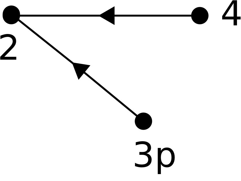
Figure 1. A component of the graph of $f$-homotopy for Hopf surfaces.

Remark 4.13.

Using the five classes of Hopf surfaces, one obtains a graph of small deformations which is more precise and complicated than the graph of $f$-homotopy, see [41], p.31. The graph of $f$-homotopy must be considered as a very rough decomposition of $\mathcal{I}$.

Example 4.14.

Hirzebruch surfaces. Consider $X=\mathbb{S}^{2}\times\mathbb{S}^{2}$. It admits complex structures of even Hirzebruch surfaces $\mathbb{F}_{2a}$. By [16], this exhausts the set of complex surfaces diffeomorphic to $X$. Then there is only one connected component of complex structures up to action of the mapping class group. The mapping class group is not known (cf. footnote 6) but contains at least four elements generated by

$$f(x,y)=(a(x),a(y))\quad\text{ and }\quad g(x,y)=(y,x).$$

where $a$ is the antipodal map of $\mathbb{S}^{2}$. Analogously to Lemma 4.11 and Corollary 4.12, we have

Lemma 4.15.

Let $\phi$ be a diffeomorphism of $X$. Assume that $\phi$ leaves a connected component of $\mathcal{I}$ invariant. Then $\phi$ is $C^{\infty}$-isotopic either to $g$ or to the identity.

Proof.

Let $J_{0}$ represent $\mathbb{P}^{1}\times\mathbb{P}^{1}$. Assume that $J_{0}\cdot\phi$ belongs to the same connected component as $J_{0}$. Then there exists a $c$-homotopy of Hirzebruch surfaces $\pi:\mathcal{X}\to[0,1]$ with endpoints $X_{0}$ and $X_{J_{0}\cdot\phi}$: just take the tautological family above a smooth path in $\mathcal{I}$ joining $J_{0}$ to $J_{0}\cdot f$. By [30, Theorem 8.1], there exists an analytic space $K$ encoding the complex structures on a neighborhood of the path and obtained by gluing together a finite number of Kuranishi spaces of Hirzebruch surfaces (up to taking the product with some vector space) such that the family $\pi$ maps onto a smooth path into $K$. Using the description of the Kuranishi spaces of Hirzebruch surfaces in [5, p.21] (see also Example 12.6), it is easy to check that

1. $K$ is a manifold.

2. The points of $K$ encoding $\mathbb{F}_{2a}$ for $a>0$ belongs to a submanifold of complex codimension at least $1$.

Hence, we may replace the initial path defining the $c$-homotopy with a new path and a thus a new $c$-homotopy with same endpoints and such that all surfaces along this path are biholomorphic to $\mathbb{P}^{1}\times\mathbb{P}^{1}$. By Fischer-Grauert’s Theorem (see [29] for the version we use), such a deformation is locally trivial, hence trivial since the base is an interval, i.e. there exists a smooth isotopy of biholomorphisms

(4.8) $$\psi_{t}\ :\ \mathbb{P}^{1}\times\mathbb{P}^{1}\to\pi^{-1}(t)\qquad(t\in[0,1])$$

In particular, $\psi_{1}\circ\psi_{0}^{-1}$ induces a biholomorphism between $X_{0}$ and $X_{J_{0}\cdot\phi}$, which is smoothly isotopic to the identity. Composing its inverse with $\phi$, this gives an automorphism of $X_{0}$, that is of $\mathbb{P}^{1}\times\mathbb{P}^{1}$, which corresponds to the same element of the mapping class group as $\phi$. Comparing with the automorphism group of $\mathbb{P}^{1}\times\mathbb{P}^{1}$ yields the result. ∎

and

Corollary 4.16.

The map (4.3) is surjective with kernel $\{[Id],[g]\}$.

Proof.

Since all Hirzebruch surfaces are $c$-homotopic, (4.3) is surjective. Lemma 4.15 gives the kernel. ∎

Now, fix a connected component $\mathcal{I}_{0}$. We want to describe it more precisely. Observe that $g$ corresponds to an automorphism of $\mathbb{P}^{1}\times\mathbb{P}^{1}$, but not of the other Hirzebruch surfaces since every automorphism of $\mathbb{F}_{2a}$ is isotopic to the identity for $a>0$. Recall that the dimension of the group of automorphism of $\mathbb{F}_{2a}$ is $2a+5$ for $a>0$, [34, p.44]. This implies

Lemma 4.17.

We have:

1. The subset $\mathcal{I}_{0}(\mathbb{F}_{0})$ of $\mathcal{I}_{0}$ consisting of structures biholomorphic to $\mathbb{P}^{1}\times\mathbb{P}^{1}$ is open and connected.

2. The closed set $\mathcal{I}_{0}\setminus\mathcal{I}_{0}(\mathbb{F}_{0})$ has exactly two connected components.

3. The diffeomorphism $g$ acts on $\mathcal{I}_{0}$ by fixing globally $\mathcal{I}_{0}(\mathbb{F}_{0})$; and by exchanging the two components of $\mathcal{I}_{0}\setminus\mathcal{I}_{0}(\mathbb{F}_{0})$.

4. Fix a connected component $\mathcal{I}_{1}$ of $\mathcal{I}_{0}\setminus\mathcal{I}_{0}(\mathbb{F}_{0})$. Then the set of points $\mathcal{I}_{2}$ encoding $\mathbb{F}_{2}$ in $\mathcal{I}_{1}$ is open and connected and its complement is connected.

5. By induction, for $a>1$, the set of points $\mathcal{I}_{a}$ encoding $\mathbb{F}_{2a}$ in $\mathcal{I}_{a-1}$ is open and connected and its complement is connected.

Proof.

Observe that $\mathcal{I}_{0}(\mathbb{F}_{0})$ is equal to $\mathcal{I}_{0}(7)$, recall (2.12). Hence it is open. Also we have already observed in the proof of Lemma 4.15 that two $c$-homotopic structures both encoding $\mathbb{P}^{1}\times\mathbb{P}^{1}$ are $c$-homotopic through a path all of whose points encode $\mathbb{P}^{1}\times\mathbb{P}^{1}$. This proves (i).
To prove (ii) and (iii), we need a variation of Lemma 4.15. Let $J_{0}$ represent $\mathbb{F}_{2}$. Call $\mathcal{I}_{1}$ the connected component of $J_{0}$ in $\mathcal{I}_{0}\setminus\mathcal{I}_{0}(\mathbb{F}_{0})$. Assume that $J_{0}\cdot\phi$ belongs to $\mathcal{I}_{1}$. Then there exists a smooth family of Hirzebruch surfaces $\pi:\mathcal{X}\to[0,1]$ with endpoints $X_{0}$ and $X_{J_{0}\cdot\phi}$ and all of whose point are distinct from $\mathbb{P}^{1}\times\mathbb{P}^{1}$. Using Theorem 8.1 of [30] and the description of the Kuranishi spaces of Hirzebruch surfaces in [5], p.21 (see also Example 12.6), it is easy to check that we may assume that all surfaces along this path are biholomorphic to $\mathbb{F}_{2}$. Arguing as in the proof of Lemma 4.15, we deduce that $\phi$ must be smoothly isotopic to the identity, since every automorphism of $\mathbb{F}_{2}$ has this property. Since we already know that $g$ fixes globally $\mathcal{I}_{0}$, this means that $J_{0}$ and $J_{0}\cdot g$ belongs to two distinct connected components of $\mathcal{I}_{0}\setminus\mathcal{I}_{0}(\mathbb{F}_{0})$ in $\mathcal{I}_{0}$.
Assume now that $J_{1}$ is another point of $\mathcal{I}_{0}$ encoding $\mathbb{F}_{2}$. Then there exists $\phi\in\text{Diff}^{+}(X)$ such that $J_{1}$ equals $J_{0}\cdot\phi$. By Corollary 4.16, $\phi$ is either isotopic to the identity or to $g$. In the first case, $J_{1}$ belongs to also to $\mathcal{I}_{1}$. In the second case, it belongs to $\mathcal{I}_{1}\cdot g$. Hence, there are exactly two connected components exchanged by $g$, and items (ii) and (iii) are proved.
Finally, similar arguments prove (iv) and (v). ∎

In other words, the associated graph of $f$-homotopy has several connected components and each connected component has two branches joined on the vertex corresponding to $\mathbb{P}^{1}\times\mathbb{P}^{1}$. Finally, each branch has a countable number of vertices, namely one vertex for each value of $a\in\mathbb{N}$. It has weight $2a+5$, except for $\mathbb{F}_{0}$ which has weight $6$. Given any $a>b$, there exists an edge from $a$ to $b$, because it is possible to deform $\mathbb{F}_{2a}$ onto $\mathbb{F}_{2b}$, cf. [5] or [34]. In particular, every vertex is attached to a countable number of edges. Similar picture is valid for the odd Hirzebruch surfaces.

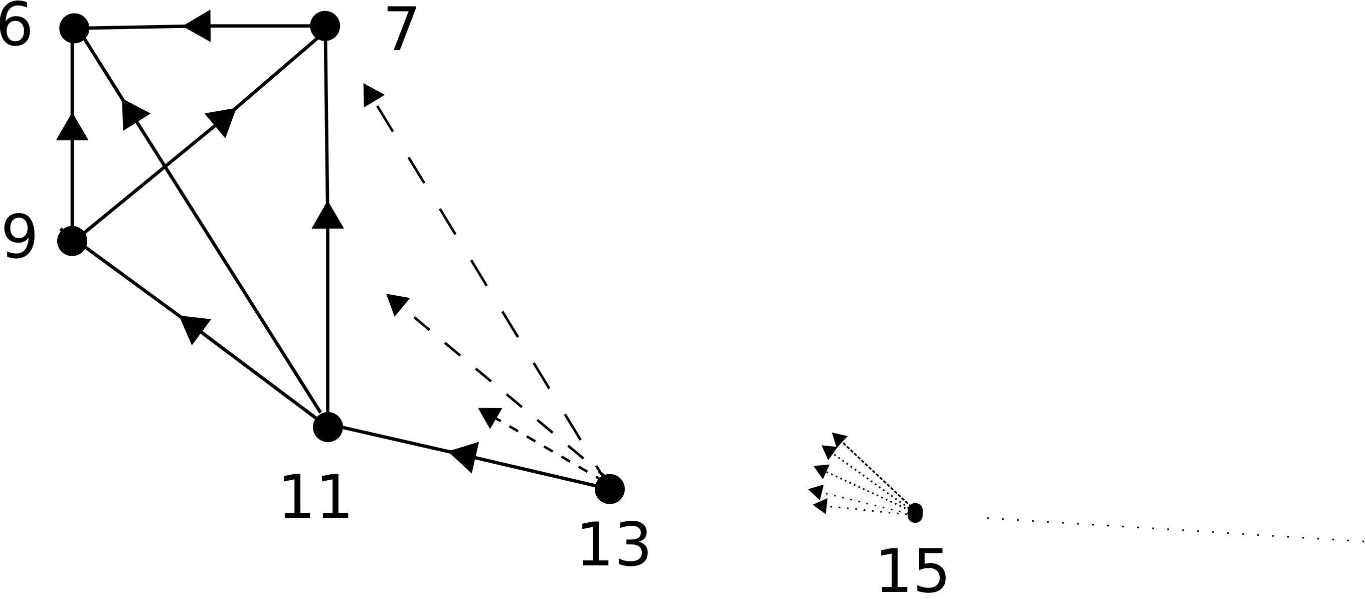
Figure 2. One of the two branches of a component of the graph of $f$-homotopy for Hirzebruch surfaces.

Remark 4.18.

Observe that the action of the mapping class group on $\mathcal{I}$ may take strongly different forms, depending on the $C^{\infty}$-manifold $X$. For $\mathbb{S}^{3}\times\mathbb{S}^{1}$, Lemma 4.11 shows that it only permutes the connected components of $\mathcal{I}$. For $\mathbb{S}^{2}\times\mathbb{S}^{2}$, some of the elements of the mapping class group permute the connected components of $\mathcal{I}$ but we also have by Lemma 4.17 an involution which fixes each component of $\mathcal{I}$. Note that this involution is isotopic to an automorphism of $\mathbb{P}^{1}\times\mathbb{P}^{1}$. The case of elliptic curves shows a different phenomenon. There is a single connected component of complex structures which is fixed by every element of the mapping class group $\text{SL}_{2}(\mathbb{Z})$. Some of them are isotopic to an automorphism of an elliptic curve, for example the multiplication by $i$; but most of them are not, cf. Example 12.1.

Remark 4.19.

Observe that in Examples 4.10 and 4.14, the Riemann moduli stack $\mathcal{M}(X)$ is connected because of Lemmas 4.11 and 4.15 (cf. Remark 4.3). However, we do not know if $\mathcal{T}(X)$ has a finite number of connected components, because it is not known if the mapping class group of $\mathbb{S}^{1}\times\mathbb{S}^{3}$, respectively $\mathbb{S}^{2}\times\mathbb{S}^{2}$, is finite or not. For example, notice that some blow ups of connected sums of $\mathbb{P}^{2}$s have infinite mapping class group, see [36].

5. The TG foliated structure of $\mathcal{I}$.

Let $\mathcal{I}_{0}$ be a connected component of $\mathcal{I}$. Assume that for all $J$ in $\mathcal{I}_{0}$, we have $h^{0}(J)$ equal to zero. Then, the action of $\text{Diff}^{0}(X)$ onto $\mathcal{I}_{0}$ is locally free and one would like to conclude that it defines a foliation of $\mathcal{I}_{0}$.

This can be made precise as follows.

Proposition 5.1.

Assume that the function $h^{0}$ is identically zero on the connected component $\mathcal{I}_{0}$. Then, the action of $\text{\rm Diff}^{0}(X)$ onto $\mathcal{I}_{0}$ induces a holomorphic foliation of $\mathcal{I}_{0}$ whose leaves are Fréchet submanifolds and whose local transverse section at a point $J$ is given by the Kuranishi space of $X_{J}$.

Remark 5.2.

Be careful that we use the word ”foliation” in an extended sense. Firstly the leaves are infinite-dimensional and secondly the transverse sections are singular spaces and are not all isomorphic. We should rather talk of ”lamination” but we prefer to reserve this terminology for foliated spaces transversely modeled onto a continuous space, e.g. a Cantor set.

Proof.

The condition that the function $h^{0}$ is zero on the whole $\mathcal{I}_{0}$ implies that, in Theorem 3.2, we may take $L_{0}$ to be the full $A^{0}$. This complex vector space is, as a real vector space, the space of vector fields $\Sigma(TX)$. Its complex structure a priori depends on the base point $J$, but it is easy to check that all $A^{0}$ are isomorphic as complex vector spaces, [30, Lemma 7.1]. Hence the isomorphisms (3.4) form a foliated atlas of $\mathcal{I}_{0}$: the plaques representing the local orbits of $\text{Diff}^{0}(X)$ are preserved by the changes of charts, cf. [30, §6]. The leaves are Fréchet submanifolds modeled onto $A^{0}$ and at a point $J$, any germ of transverse section is isomorphic to the Kuranishi space of $X_{J}$. ∎

In the general case, we think of Kuranishi Theorem 3.2 as describing a foliated structure on $\mathcal{I}$ which is no more transversally modelled onto an analytic space as in Proposition 5.1 but on the Kuranishi stack of section 3.2. In previous versions of this paper, we formalize this structure as a TG foliation, but the definition we gave is not completely satisfactory. There are several technical issues with it and solving them is unrelated to our results, so we prefer replacing it with the notion of TG foliated structure which is a purely transverse notion. We set

Definition 5.3.

By TG foliated structure of $\mathcal{I}$, we mean a collection of Kuranishi stacks associated to a collection of Kuranishi domains which cover the whole space $\mathcal{I}$.

We think of it as a collection of local transversals to the $\text{\rm Diff}^{0}(X)$-action.

6. The holonomy groupoid of the TG foliated structure of $\mathcal{I}$.

Let $\mathcal{F}$ be a foliation of some analytic space. We may associate to it a holonomy groupoid as follows ([32, §5.2] and [17]). We choose a set of local transverse sections. Objects of the groupoid are points of the disjoint union of these local sections. Morphisms are generated by holonomy morphisms, obtained by following the leaves from a transverse section to another one, identifying holonomy morphisms having the same germ. It is an étale groupoid, which encodes the leaf space of the foliation.
Having proved in Proposition 5.1 that the action of $\text{Diff}^{0}(X)$ induces a foliation of each connected component of $\mathcal{I}$ when $h^{0}$ is equal to zero, and considering in the general case the TG foliated structure of $\mathcal{I}$, we would like to associate to this TG foliated structure a holonomy groupoid. As in the classical case, it should be a presentation of the quotient stack, that is here of the Teichmüller stack.
However, this is much more involved than in the classical case. The problem is that now the transverse sections are modelled onto groupoids (3.10), so that holonomy morphisms are stacks morphisms between Kuranishi stacks. Hence, if we just follow the same strategy, instead of building a groupoid, we end with a disjoint union of stacks and a set of local stack morphisms. It is certainly possible to turn this collection into a nice categorical structure. However, we will not follow this path since we are interested in obtaining a presentation of the Teichmüller stack. The crucial point is to lift holonomy morphisms between Kuranishi stacks to morphisms between Kuranishi spaces.
This lifting process will be done in four steps, in sections 8, 9 and 11.
Firstly in section 8, we construct partial foliations of $\mathcal{I}_{0}$. Partial here means that they are not defined on the whole $\mathcal{I}_{0}$ but on an open subset. We take a countable collection of such foliations whose domains of definition cover $\mathcal{I}_{0}$. Basically, the transverse structure of these foliations at some point $J$ is modeled onto the Kuranishi space of the corresponding complex manifold $X_{J}$. However, the jumps in the dimension of the automorphism group cause serious problems here, and we start doing the construction in the neighborhood of a $f$-homotopy class, where equidimensionality is fulfilled. Then we extend it to the whole $\mathcal{I}_{0}$, but to achieve that, we are forced to fat the smallest Kuranishi spaces to finish with all transversals of the same dimension. This fatting process was already used in [30].
Secondly, from this set of partial foliations, we define regular atlases for this multifoliation and simple holonomy germs as the classical holonomy germs of each partial foliation. The main point is that we allow, under certain circumstancies, composition of holonomy germs coming from two different foliations. The peculiarities of a regular atlas are useful in this process. We encode all the holonomy data related to a regular atlas in a groupoid. This is however not the good groupoid to consider, especially because changing of regular atlas does not produce a Morita equivalent groupoid. All this is done in subsections 9.1, 9.2 and 9.3. This preliminary work is essentially notational and technical, but is important to achieve the construction.
Thirdly, building on the previous sections, we construct in subsection 9.4 the holonomy groupoid of the TG foliated structure of $\mathcal{I}_{0}$. We call it the Teichmüller groupoid. Its objects are points of a disjoint union of transverse sections of partial foliations covering $\mathcal{I}_{0}$. Its morphisms are composition of the simple holonomy germs and of morphisms of type (3.9) on its Kuranishi space, up to an equivalence relation.
Fourthly, and last, we prove that the Teichmüller groupoid is an analytic smooth groupoid and a presentation of the Teichmüller stack in Theorem 11.1, which implies Theorem 2.9. Basically there are two points to check. From the one hand, it must be shown that composition of simple holonomy germs and local automorphisms describes the full action of $\text{Diff}^{0}(X)$ onto $\mathcal{I}_{0}$. This is done in Lemma 11.3. From the other hand, it must be shown that the source and target maps are smooth morphisms. This is essentially an adaptation of the arguments involved in the proof of Lemma 3.12. Analogously, we prove Theorem 11.8, which implies Theorem 2.10.
Before developing all this construction, we consider in the next section the rigidified case, in which the TG foliated structure comes from a foliation, and the Teichmüller groupoid an ordinary holonomy groupoid. This can be seen as a toy model for the general construction and will serve to fixing some notations and conventions.

7. The rigidified case.

Recall the

Definition 7.1.

(see [7], Definition 12). A compact complex manifold $X_{J}$ is rigidified if $\text{Aut}^{1}(X_{J})$ is equal to the identity.

In that case, the map

(7.1) $$f\in\text{Diff}^{0}(X)\longmapsto J\cdot f\in\mathcal{I}$$

is injective. Moreover,

Proposition 7.2.

Assume that all structures of some connected component $\mathcal{I}_{0}$ are rigidified. Then, the action of $\text{\rm Diff}^{0}(X)$ onto $\mathcal{I}$ is free and defines a foliation of $\mathcal{I}_{0}$ whose leaves are Fréchet manifolds modelled onto the vector space of smooth sections of $TX$ and with local transversal $K_{0}$ at $J_{0}$.

Proof.

Freeness is immediate from (7.1). The foliation is that of Proposition 5.1. ∎

In the case of Proposition 7.2, the Teichmüller groupoid is just the standard holonomy groupoid of the foliation. We give now a complete treatment of this case, which serves as a toy model for section 9. We cover $\mathcal{I}_{0}$ by a collection $(U_{\alpha})_{\alpha\in A}$ of open subsets. We assume that each chart $U_{\alpha}$ is a Kuranishi domain satisfying hypothesis 3.5 associated to the following retraction map (the composition is the identity, cf. (3.6))

(7.2) $$\begin{CD}K_{\alpha}\hookrightarrow U_{\alpha}@>{\Xi_{\alpha}}>{}>K_{\alpha}\end{CD}$$

We denote by $J_{\alpha}$ the base point of the Kuranishi space $K_{\alpha}$. Observe that the index set may be assumed to be countable, due to Proposition 4.2 and the countability of the involved topologies.
Take two points $x\in K_{\alpha}$ and $y\in K_{\beta}$ belonging to the same leaf and choose a path of foliated charts joining $x$ to $y$. A holonomy germ from $x$ to $y$ is a germ of analytic isomorphism between the pointed spaces $(K_{\alpha},x)$ and $(K_{\beta},y)$, which is obtained by identifying along the path of foliated charts points belonging to the same leaf, see [32, §2.1] or [9].
They can be encoded in a holonomy groupoid [32, §5.2] or [17] as follows. Objects are points of the disjoint union of transversals

(7.3) $$\mathop{\bigsqcup}_{\alpha\in A}K_{\alpha}.$$

We denote by $(x,\alpha)$ a point of $K_{\alpha}$. To encode the morphisms, we first notice that on each non-empty intersection $U_{\alpha}\cap U_{\beta}$, there exists a unique isomorphism $\phi_{\alpha,\beta}$ between some open subset $K_{\alpha,\beta}$ of $K_{\alpha}$ and some open subset $K_{\beta,\alpha}$ of $K_{\beta}$. It is obtained by following the leaves of the foliation from $K_{\alpha}$ till meeting $K_{\beta}$ (when this occurs). It satisfies the commutative diagram

(7.4) $$\begin{CD}U_{\alpha}\cap U_{\beta}@>{Id}>{}>U_{\alpha}\cap U_{\beta}\cr @V{\Xi_{\alpha}}V{}V@ VV\Xi_{\beta}V\cr K_{\alpha,\beta}@>{\simeq}>{\phi_{\alpha,\beta}}>K_{\beta,\alpha}\end{CD}$$

Remark 7.3.

It happens that Kuranishi spaces are everywhere non-reduced. Hence a morphism between Kuranishi spaces is not completely determined by its values, the values of its differential must also be prescribed. The previous definition of $\phi_{\alpha,\beta}$ by following the leaves just determines its values. However, since $\Xi_{\alpha}$ and $\Xi_{\beta}$ are smooth morphisms by Kuranishi’s Theorem 3.2, the equality $d\phi_{\alpha,\beta}\circ d\Xi_{\alpha}=d\Xi_{\beta}$ coming from (7.4) determines the values of its differential. Thus, even in this non-reduced situation, we have completely and uniquely defined the isomorphism $\phi_{\alpha,\beta}$ making (7.4) commutative.

We now look at the groupoid of germs generated by the $\phi_{\alpha,\beta}$. In other words, we now let $(\alpha_{1},\ldots,\alpha_{n})$ be a collection of indices such that each $U_{\alpha_{i}}\cap U_{\alpha_{i+1}}$ is non-empty and define

(7.5) $$\phi_{\alpha_{1},\ldots,\alpha_{n}}:=\phi_{\alpha_{n-1},\alpha_{n}}\circ\ldots\circ\phi_{\alpha_{1},\alpha_{2}}.$$

This composition is defined on some open subset of $K_{\alpha_{1}}$ that we denote by $K_{\alpha_{1},\ldots,\alpha_{n}}$; and it ranges in some open subset of $K_{\alpha_{n}}$, that we denote by $K_{\alpha_{n},\ldots,\alpha_{1}}$. Then we represent all holonomy maps as points of

(7.6) $$\mathop{\bigsqcup}_{n\geq 1}\left(\mathop{\bigsqcup}_{(\alpha_{1},\ldots,\alpha_{n})\in B_{n}}K_{\alpha_{1},\ldots,\alpha_{n}}\right).$$

Here $(\alpha_{1},\ldots,\alpha_{n})\in B_{n}$ if each $U_{\alpha_{i}}\cap U_{\alpha_{i+1}}$ is non-empty. A point $x$ in some $K_{\alpha_{1},\ldots,\alpha_{n}}$ represents the germ at $x$ of the map $\phi_{\alpha_{1},\ldots,\alpha_{n}}$, the case $n=1$ encoding the identity germs. We denote such a point by the $(n+1)$-uple $(x,\alpha_{1},\ldots,\alpha_{n})$.
Consider the groupoid whose objects are given in (7.3), and morphisms are given in (7.6). Observe that both sets are $\mathbb{C}$-analytic spaces. The source map sends $(x,\alpha_{1},\ldots\alpha_{n})$ onto $(x,\alpha_{1})$ and the target map sends it to $(\phi_{\alpha_{1},\ldots,\alpha_{n}}(x),\alpha_{n})$. Both are obviously étale analytic maps, since the source map is just the inclusion $K_{\alpha_{1},\ldots,\alpha_{n}}\subset K_{\alpha_{1}}$ on the component $K_{\alpha_{1},\ldots,\alpha_{n}}$; and the target map on the same component is the composition of the isomorphism $\phi_{\alpha_{1},\ldots,\alpha_{n}}$ from $K_{\alpha_{1},\ldots,\alpha_{n}}$ onto $K_{\alpha_{n},\ldots,\alpha_{1}}$ with the inclusion $K_{\alpha_{n},\ldots,\alpha_{1}}\subset K_{\alpha_{n}}$. Multiplication is given by composition of holonomy germs.
However, we are not finished yet. The previous groupoid is not the holonomy groupoid of the foliation. We must still identify identical germs. It may happen for example that such a composition $\phi_{\alpha_{1},\ldots,\alpha_{n}}$ is the identity. So we take the quotient of (7.6) by the following equivalence relation

(7.7) $$(x,\alpha)\sim(x^{\prime},\alpha^{\prime})\iff\left\{\begin{aligned} &x=x^{\prime},\ \alpha_{1}=\alpha^{\prime}_{1},\ \alpha_{n}=\alpha^{\prime}_{n^{\prime}}\cr\text{and }&\big{(}\phi_{\alpha_{1},\ldots,\alpha_{n}}\big{)}_{x^{\prime}}\equiv\big{(}\phi_{\alpha^{\prime}_{1},\ldots,\alpha^{\prime}_{n^{\prime}}}\big{)}_{x}\end{aligned}\right.$$

that is if they have same source, same target, and are equal as germs. Hence, the set of morphisms is

(7.8) $$\mathop{\bigsqcup}_{n\geq 1}\left(\mathop{\bigsqcup}_{(\alpha_{1},\ldots,\alpha_{n})\in B_{n}}K_{\alpha_{1},\ldots,\alpha_{n}}\right)\Biggm{/}\sim$$

We set

Definition 7.4.

We call Teichmüller groupoid of $\mathcal{I}_{0}$ the groupoid whose objects are given by (7.3), whose morphisms are given in (7.8), and whose source, target maps and multiplication are defined as above.

We define in the same way the Teichmüller groupoid of $V$, an open subset of $\mathcal{I}$.

Proposition 7.5.

The Teichmüller groupoid is an analytic étale groupoid.

Proof.

From the above discussion, we just have to prove that (7.8) is still an analytic space and that the projection map from (7.6) onto (7.8) is étale.

Observe that two distinct points of the same component $K_{\alpha_{1},\ldots,\alpha_{n}}$ of (7.6) cannot be equivalent. Therefore, the natural projection map from (7.6) onto (7.8) is étale and we just have to show that (7.8) is Hausdorff to finish with the proof.

This comes from a standard argument, cf. [4, prop. 3.2]. Consider two equivalent convergent sequences $(x_{p},\alpha_{p})$ and $(x_{p},\alpha^{\prime}_{p})$. We may assume that all $\alpha_{p}$, resp. $\alpha^{\prime}_{p}$, are the same, say $\alpha$, resp. $\alpha^{\prime}$. Assume that $(x_{p})$ converges to $x$. Then this means that $\big{(}\phi^{-1}_{\alpha_{1},\ldots,\alpha_{n}}\circ\phi_{\alpha^{\prime}_{1},\ldots,\alpha^{\prime}_{n}}\big{)}_{x_{p}}\equiv Id_{x_{p}}$, i.e. the germ of this morphism is the identity at every point $x_{p}$. By analyticity, this implies that it is also the identity at the limit point $x$. ∎

Remark 7.6.

The construction above depends on a choice of a foliated atlas. However, it is easy to show that it is independent of this choice up to Morita equivalence. This can of course be deduced from general arguments, since it represents the stack $\mathcal{T}(X,\mathcal{I}_{0})$, which does not depend on a foliated atlas. It can also be proved directly as follows. Start with a foliated atlas and construct the associated Teichmüller groupoid. Take a finer foliated atlas. Then the associated Teichmüller groupoid is just the localization of the first one over the new atlas, hence both are weakly equivalent [17]. Start now with two different foliated atlases and their associated Teichmüller groupoid. Since the union of the atlases is a common refinement of both of them, the two groupoids are Morita equivalent.

Remark 7.7.

Assume that for all structures $J$ in $\mathcal{I}_{0}$, we have $\text{Aut}^{0}(X_{J})$ equal to the identity. Then Proposition 5.1 still applies and the action of $\text{Diff}^{0}(X)$ still defines a foliation of $\mathcal{I}_{0}$. So we can still define a holonomy groupoid as above. Morover the geometric quotient of the Teichmüller stack equals the leaf space, that is the geometric quotient of this holonomy groupoid. Nevertheless, they may be different as stacks, because there may exist a non trivial element in $\text{Aut}^{1}(X_{J})$ that fixes $\mathcal{I}_{0}$. Such an element is encoded in the Teichmüller groupoid we construct in section 9 but not in the holonomy groupoid of Definition 7.4, cf. Remark 9.15.
For many compact complex manifolds $X_{0}$, there is no difference between $\text{Aut}^{0}(X_{0})$ and $\text{Aut}^{1}(X_{0})$, cf. [7]. We gave an example of $X_{0}$ with $\text{\rm Aut}^{0}(X_{0})$ and $\text{\rm Aut}^{1}(X_{0})$ distinct in [31]. The dimension of $\text{\rm Aut}^{0}(X_{0})$ is positive so this leads to the following problem.

Problem 7.8.

Find a compact complex manifold $X_{0}$ with $\text{Aut}^{0}(X_{0})$ being reduced to the identity but which is not rigidified.

If $X_{0}$ is Kähler, then a result of Liebermann implies that $\text{Aut}^{0}(X_{0})$ has finite index in $\text{Aut}^{1}(X_{0})$. In the non-Kähler case, however, there should even exist examples with infinite ”complex mapping class group” $\text{Aut}^{1}(X_{0})/\text{Aut}^{0}(X_{0})$.

8. The set of partial foliated structures of $\mathcal{I}$.

In this section, we associate to the TG foliated structure of a connected component $\mathcal{I}_{0}$ of $\mathcal{I}$ a collection of standard foliations of open sets of $\mathcal{I}_{0}$ covering it. In subsection 9.2, we will associate to these partial foliations their holonomy germs. This is a crucial step in defining the morphisms of the Teichmüller groupoid. The main problem here is that the dimension of the Kuranishi spaces may vary inside $\mathcal{I}_{0}$. To overcome this difficulty, we proceed in two steps. It turns out that the dimension we have really to care about in this problem is the dimension of the automorphism group. Hence we first work in the neighborhood of a $f$-homotopy class, so that we may assume equidimension of the automorphism groups involved in the choice of foliated atlases. Then, we treat the general case. We have to fat the Kuranishi spaces with small automorphism group, following a process already used in [30]. This supposes the function $h^{0}$ to be bounded on $\mathcal{I}_{0}$.

8.1. The set of partial foliated structures of a neighborhood of a $f$-homotopy class.

Let $\mathcal{F}$ be a $f$-homotopy class in $\mathcal{I}$. Let $V$ be a connected neighborhood of $\mathcal{F}$ in $\mathcal{I}_{0}$. Let $G(\Sigma(TX))$ be the grassmannian of closed vector subspaces of $\Sigma(TX)$ of codimension $h^{0}(\mathcal{F})$. For each $L\in G(\Sigma(TX))$, define

(8.1) $$\mathcal{F}_{L}=\{J\in\mathcal{F}\mid L\oplus\text{Re }H^{0}(X_{J},\Theta_{J})=\Sigma(TX)\}.$$

Definition 8.1.

We say that $L$ is $\mathcal{F}$-admissible if $\mathcal{F}_{L}$ is not empty.

Assume that $L$ is $\mathcal{F}$-admissible and let $J_{0}\in\mathcal{F}_{L}$. Then, using the isomorphism

(8.2) $$\xi\in A^{0}\longmapsto\xi+\bar{\xi}\in\Sigma(TX)$$

(where $A^{0}$ is the space of $(1,0)$-vectors for the structure $J_{0}$), we see that the choice of a $\mathcal{F}$-admissible $L$ is equivalent to the choice of a closed subspace $L_{0}$ of $A^{0}$ satisfying (3.3) and

(8.3) $$\text{Re }L_{0}=L.$$

In the sequel, we will denote by the same symbol $L$ a closed subspace of $A^{0}$ and its real part in $\Sigma(TX)$. No confusion should arise from this abuse of notation. Observe that all such $L$ are complex isomorphic, cf. [30, Lemma 7.1].
So, once chosen such an $L$, we may apply Theorem 3.2 at $J_{0}$ with $L$. We define $V_{L}$ as the maximal open subset of $V$ covered by Kuranishi domains modelled on $L$ and based at points of $\mathcal{F}_{L}$. We can interpretate it as follows. Theorem 3.2 endows each Kuranishi domain with a trivial local foliation by copies of $L$ and leaf space $K_{0}$.
Now, let us put this interpretation in a global setting. It tells us that we may cover $V_{L}$ by Kuranishi domains modelled on the same $L$. Hence $L$ defines a foliation of $V_{L}$ by leaves locally isomorphic to a neighborhood of $0$ in $L$, see [30, Theorem 7.2].

Definition 8.2.

We call this foliation the $L$-foliation of $V$ (even if it is only defined on $V_{L}$).

In the case where $V_{L}$ is equal to $V$, which is equivalent to saying that $L$ is a common complement to all $H^{0}(X_{J},\Theta_{J})$ for $J\in\mathcal{F}$, then we obtain a global foliation of $V$.
Nevertheless, it is not possible in general to assume this hypothesis. Hence we shall replace this foliated structure by a collection of partial foliations encoded in a groupoid.

Definition 8.3.

A set $\mathcal{L}$ of $\mathcal{F}$-admissible elements of $G(\Sigma(TX))$ such that

(8.4) $$\mathop{\bigcup}_{L\in\mathcal{L}}V_{L}=V.$$

is called a covering family of $V$.

Choose $\mathcal{L}$ a covering family of $\mathcal{F}$. Observe that we may assume $\mathcal{L}$ to be countable by Proposition 4.1. To $\mathcal{L}$ is associated a covering set of partial foliations of $V$, defined as the set of all $L$-foliations of $V$ for $L\in\mathcal{L}$. It is useful to encode it in a groupoid as follows.
For each $L\in\mathcal{L}$, choose an atlas

(8.5) $$\mathcal{U}_{L}=(U_{\alpha})_{\alpha\in A_{L}}$$

of $V_{L}$ by $L$-foliated charts satisfying hypothesis 3.5. Define

(8.6) $$A=\mathop{\bigsqcup}_{L\in\mathcal{L}}A_{L}\qquad\text{ and }\qquad\mathcal{U}=(\mathcal{U}_{L})_{L\in\mathcal{L}}$$

Once again, we may assume that $A$ is countable, due to the countability of the involved topologies. Then define the groupoid $G_{\mathcal{U}}$ as follows. Objects are points of the disjoint union

(8.7) $$\mathop{\bigsqcup}_{\alpha\in A}U_{\alpha}$$

hence are encoded by couples $(x,\alpha)$.
We insist on seeing each $U_{\alpha}$ as a $L$-foliated Fréchet space. We use the notation

(8.8) $$L\in\alpha$$

to denote the vector space $L$ associated to $\alpha$. In section 9, we will enlarge our index set $A$ and the interest of this strange notation should be clarified. Set now

(8.9) $$B=\mathop{\bigsqcup}_{L\in\mathcal{L}}B_{L}=\mathop{\bigsqcup}_{L\in\mathcal{L}}\{(\alpha,\beta)\in A^{2}\mid\alpha\not=\beta,\ L\in\alpha\text{ and }L\in\beta\}.$$

Morphisms are points

(8.10) $$\mathop{\bigsqcup}_{\alpha\in A}U_{\alpha}\mathop{\bigsqcup}_{(\alpha,\beta)\in B}U_{\alpha}\cap U_{\beta}$$

encoded by triples $(x,\alpha,\beta)$.
Once again, we insist on seeing each $U_{\alpha}\cap U_{\beta}$ as a $L$-foliated Fréchet space. Note that there is no morphism between a point in a $L$-foliated chart and the same point in a $L^{\prime}$-foliated chart.

8.2. The general case.

We now deal with the definition of a covering set of partial foliations and its encoding in a groupoid for all points of $\mathcal{I}_{0}$ with bounded function $h^{0}$.
Let $a\in\mathbb{N}$. Recall (2.12). Recall that $\mathcal{I}(a)$ is open. We assume that it is connected, replacing it with a connected component otherwise. Given a closed subspace $L$ of $\Sigma(TX)$ of codimension $a$, define

(8.11) $$\mathcal{F}_{L}=\{J\in\mathcal{I}_{0}(a)\mid L\cap\text{Re }H^{0}(X_{J},\Theta_{J})=\{0\}\}.$$

This is an extension of (8.1). We may go on with this generalization.

Definition 8.4.

We say that $L$ is $a$-admissible if $\mathcal{F}_{L}$ is not empty.

Analogously to what happens in subsection 8.1, the choice of an $a$-admissible $L$ is equivalent to the choice of a closed subspace $L_{0}$ of $A^{0}$ satisfying

(8.12) $$L_{0}\cap H^{0}(X_{J},\Theta_{J})=\{0\}\quad\text{ and }\quad\text{Re }L_{0}=L.$$

As in subsection 8.1, we denote both $L$ and $L_{0}$ by the same symbol $L$. Although this $L$ is not a complement of $H^{0}(X_{J},\Theta_{J})$, we may run the proof of Kuranishi’s Theorem after adding some finite-dimensional subspace $H_{L}$ such that

(8.13) $$L\oplus H_{L}\oplus H^{0}(X_{J},\Theta_{J})=A^{0}.$$

Remark 8.5.

We assume that $H_{L}$ contains only $C^{\infty}$ elements, so that we may use the same $H_{L}$ for all Sobolev classes. This is always possible by perturbing a little a basis of $H_{L}$ since $C^{\infty}$ diffeomorphisms are dense in $L^{2}_{l}$ diffeomorphisms for $l$ big enough.

We thus obtain an isomorphism between a neighborhood $U$ of $J$ in $\mathcal{I}$ and a product (cf. [30, Theorem 7.2])

(8.14) $$\begin{CD}U@ >\Phi:=(\Xi,\Upsilon)>>(K_{J}\times H_{L})\times L.\end{CD}$$

whose inverse is given by

(8.15) $$(J,\xi,\xi^{\prime})\in\Phi(U)\cap(K_{J}\times H_{L}\times L)\longmapsto(J\cdot e(\xi))\cdot e(\xi^{\prime})$$

Setting

(8.16) $$K:=\Phi(U)\subset K_{J}\times H_{L}$$

we obtain a sequence analogous to (7.2)

(8.17) $$\begin{CD}K\hookrightarrow U@>{\Xi}>{}>K.\end{CD}$$

This is our new definition of Kuranishi domains and charts. We replace hypothesis (3.5) with

Hypothesis 8.6.

The image of $\Phi$ is contained in a product $K\times(W^{\prime}\cap L)=K_{J}\times(W^{\prime}\cap H_{L})\times(W^{\prime}\cap L)$ with $W^{\prime}\subset W$ an open and connected neighborhood of $0$ in $A^{0}$.

Let $\mathcal{U}$ be a covering of $\mathcal{I}_{0}(a)$ by Kuranishi domains satisfying hypothesis 8.6. Set $V=\mathcal{I}_{0}(a)$. We define $V_{L}$ as the maximal open subset of $V$ covered by Kuranishi domains satisfying hypothesis 8.6, modelled on $L$ and based at points of $\mathcal{I}_{0}(a)$. We may then define the sets of objects and morphisms of the groupoid $G_{\mathcal{U}}$ of partial foliations of $V$ exactly as in subsection 8.1. The structure maps are the obvious ones (cf. the proof of Proposition 8.9).

Remark 8.7.

Recall that the local transversal section at some point $J_{0}$ is not always its Kuranishi space $K_{0}$. It is if and only if $h^{0}(J_{0})$ is equal to $a$. More generally, it is the product of $K_{0}$ with an open neighborhood of $0$ in $\mathbb{C}^{a-h^{0}(J_{0})}$.

Remark 8.8.

Observe that, if the function $h^{0}$ is bounded on a connected component $\mathcal{I}_{0}$ by some integer $a$, then $\mathcal{I}_{0}(a)$ is equal to $\mathcal{I}_{0}$.

8.3. Properties of the groupoid of partial foliated structures.

The following Proposition shows that the groupoid of partial foliated structures really describes an intrinsic geometric structure.

Proposition 8.9.

We have:
I. The groupoid $G_{\mathcal{U}}$ is a foliated Fréchet étale groupoid, that is

1. Both the set of objects and that of morphisms are foliated Fréchet manifolds.

2. The source, target, composition, inverse and anchor maps are analytic and respects the foliations.

3. The source and target maps are local foliated isomorphisms.

II. The foliated Fréchet groupoid $G_{\mathcal{U}}$ is independent of $\mathcal{U}$ up to foliated analytic Morita equivalence.

Proof.

This is completely standard, since this groupoid is very close to the Lie groupoid obtained by localization of a smooth manifold over an atlas, see [13], §7.1.3. Starting with I, then (i) is obvious from (8.7) and (8.10); the source map $\sigma$ and the target map $\tau$ are given by the following foliation preserving inclusions

(8.18) $$\begin{CD}U_{\alpha}@<{\sigma}<{}<U_{\alpha}\cap U_{\beta}@>{\tau}>{}>U_{\beta}\end{CD}$$

proving (iii) and part of (ii). Composition is given by

(8.19) $$(x,\alpha,\beta)\times(x,\beta,\gamma)\longmapsto(x,\alpha,\gamma)$$

provided that

$$L\in\alpha\cap\beta\cap\gamma$$

(the notation should be clear from (8.8)). Assume for simplicity that $\alpha$, $\beta$ and $\gamma$ are pairwise distinct. This is indeed a foliation preserving analytic map from

$$\{(\phi,\psi)\text{ morphisms of }G_{\mathcal{U}}\mid\tau(\phi)=\sigma(\psi)\}$$

that is

(8.20) $$\mathop{\bigsqcup}_{(\alpha,\beta,\beta,\gamma)\in\sqcup{B_{L}}^{2}}U_{\alpha}\cap U_{\beta}\cap U_{\gamma}$$

onto (8.10). Other cases are treated similarly. This finishes the proof of (ii), hence of I.
As for II, start from choosing two coverings $\mathcal{U}$ and $\mathcal{V}$ of $V$. The crucial point is contained in I: these groupoids are étale. From that, it is enough to observe that both the localization of $G_{\mathcal{U}}$ over $\mathcal{V}$ and the localization of $G_{\mathcal{V}}$ over $\mathcal{U}$ are equal to the groupoid $G_{\mathcal{U}\cap\mathcal{V}}$ (see [17] for the equivalence with the classical definition of Morita equivalence). ∎

To finish this section, we note that $G_{\mathcal{U}}$ encodes all the possible foliations of open sets of $V$ associated to Kuranishi domains. Indeed we have

Proposition 8.10.

The full subgroupoid of $G_{\mathcal{U}}$ obtained by restriction to a fixed $L\in\mathcal{L}$ is the localization over some atlas $V_{L}$, hence is Morita equivalent to the largest subdomain of $V$ foliated by $L$.

9. The Teichmüller groupoid.

In this section, we construct for the TG foliated structure of $\mathcal{I}_{0}$ the analogue for the holonomy groupoid. We call it the Teichmüller groupoid. This will be done in several steps. In subsection 9.1, we first give a sort of foliated atlas of $\mathcal{I}_{0}$ with good properties. We call it a regular atlas. We then define in subsection 9.2 the holonomy germs associated to the set of partial foliations. In subsection 9.3, we encode these simple holonomy morphisms in a groupoid $K_{\mathcal{U}}$. This is however not the right analogue for the holonomy groupoid, since it does not take into account the isotropy groups of the transverse structure of the TG foliated structure. From the regular atlas, we finally build in subsection 9.4 the Teichmüller groupoid.

9.1. Regular atlases.

We need to construct on $V$ an equidimensional atlas from the atlas $\mathcal{U}$ of $K_{\mathcal{U}}$. Besides, we need this atlas to reflect the partial foliated structure of $\mathcal{I}_{0}$ to be able to define properly the holonomy germs.
As in section 8, we fix $\mathcal{L}$ and we define (8.5) and (8.6) as well as $G_{\mathcal{U}}$.
We assume that each chart $U_{\alpha}$ is a Kuranishi domain satisfying hypothesis 8.6, based at $J_{\alpha}$ and associated to the following retraction map (the composition is the identity, cf. (8.17))

(9.1) $$\begin{CD}K_{\alpha}\hookrightarrow U_{\alpha}@>{\Xi_{\alpha}}>{}>K_{\alpha}\end{CD}$$

Recall Remark 8.7.
The set of holonomy germs of $G_{\mathcal{U}}$ is constructed from the union of all holonomy groupoids when $L$ varies. But in order to mix these holonomies, we first add some charts with common transversal for different foliations. More precisely, for every couple $(L,L^{\prime})$ in $\mathcal{L}^{2}$ with

(9.2) $$V_{L}\cap V_{L^{\prime}}\not=\emptyset$$

we enlarge the index set $A$ to include new indices $\alpha$ and new charts

(9.3) $$\begin{CD}K_{\alpha}@<{\Xi_{\alpha,L}}<{}<U_{\alpha,L}\quad\text{ and }\quad U_{\alpha,L^{\prime}}@>{\Xi_{\alpha,L^{\prime}}}>{}>K_{\alpha}\end{CD}$$

which cover (9.2). We emphasize that the same analytic set $K_{\alpha}$ is used as leaf space for both the $L$ and the $L^{\prime}$-foliations. This is possible due to the uniqueness properties in Kuranishi’s Theorem 3.2.
In the same way, for any value of $n\geq 3$, we enlarge the index set $A$ to include new indices and charts

(9.4) $$\begin{CD}U_{\alpha,L_{i}}@>{\Xi_{\alpha,L_{i}}}>{}>K_{\alpha}\end{CD}$$

for $i=1,\ldots,n$, covering

(9.5) $$V_{L_{1}}\cap\ldots\cap V_{L_{n}}\not=\emptyset.$$

Once again, we insist on the fact that $K_{\alpha}$ is a common leaf space for every $L_{i}$-foliation restricted to $U_{\alpha,L_{i}}$. We use the notation

(9.6) $$L_{i}\in\alpha\qquad\text{ for all }\qquad i=1,\ldots,n$$

as a natural extension of (8.8).
All new charts are supposed to satisfy 8.6. We define

Definition 9.1.

We call regular atlas of $V$ such a foliated atlas $\mathcal{U}$.

Remark 9.2.

It is important to notice that the new covering $\mathcal{U}$ is constructed from the covering $\mathcal{U}$ of $G_{\mathcal{U}}$ but has strictly more charts because of (9.4) and (9.3). Moreover, this (extended) covering cannot be used to construct some $G_{\mathcal{U}}$, since each chart of $G_{\mathcal{U}}$ has to be explicitely associated to a unique $L\in\mathcal{L}$. However, to avoid cumbersome notations, we use the same symbol for both coverings.

We have now to pay attention to the fact that $K_{\alpha}$ is no more the Kuranishi space of $J_{\alpha}$, but its product with some open set in $H_{L}\simeq\mathbb{C}^{a-h^{0}(J_{\alpha})}$, cf. (8.14). Hence the groupoid (3.10) of subsection 3.2 is not the good one to consider. This can be easily fixed by fatting also the group $\text{\rm Aut}^{0}(X_{0})$. Recall (8.13) and Remark 8.5.

The following generalization of Lemmas 3.8 and 3.11 is straightforward to prove.

Lemma 9.3.

We have

1. If $W^{\prime}\subset W$ is small enough, then there exist an open and connected neighborhood $T_{\alpha}$ of the identity in $\text{\rm Aut}^{0}(X_{\alpha})$ and an open and connected neighborhood $D_{\alpha,L}$ of the identity in $\text{\rm Diff}^{0}(X)$ such that

   (9.7) $$(\xi,\xi^{\prime},g)\in W^{\prime}\cap H_{L}\cap W^{\prime}\cap L\times T_{\alpha}\longmapsto g\circ e(\xi)\circ e(\xi^{\prime})\in D_{\alpha,L}$$

   is an isomorphism.

2. Set $\mathcal{D}_{\alpha,L}=\bigcup_{g\in\text{\rm Aut}^{0}(X_{\alpha})}gD_{\alpha,L}$. Then (9.7) extends as an isomorphism

   (9.8) $$(\xi,\xi^{\prime},g)\in W^{\prime}\cap H_{L}\cap W^{\prime}\cap L\times\text{\rm Aut}^{0}(X_{\alpha})\longmapsto g\circ e(\xi)\circ e(\xi^{\prime})\in\mathcal{D}_{\alpha,L}$$

3. Both (9.7) and (9.8) extend to analytic isomorphisms of the Sobolev completions.

Now define

(9.9) $$G_{\alpha}:=\{g\circ e(\xi)\mid(g,\xi)\in\text{Aut}^{0}(X_{\alpha})\times(H_{L}\cap W^{\prime})\}$$

Remark 9.4.

Be careful that $G_{\alpha}$ is not a group, just a fatting of $\text{Aut}^{0}(X_{\alpha})$.

We let $g\in G_{\alpha}$ act on $K_{\alpha}$ exactly as in (3.9), that is

(9.10) $$xg:=\Xi_{\alpha,L}(x\cdot g)$$

and form the corresponding groupoid $\mathcal{A}_{\alpha,L}\rightrightarrows K_{\alpha}$ as in section 3.2. Notice that (9.10) depends on a choice of $L$.

9.2. Simple holonomy morphisms.

In this subsection, we associate to the partial foliations of $\mathcal{I}_{0}$ their holonomy germs. The main point is how to mix the holonomies of the different foliations. We refer to section 7 for comparison.
We start with a regular atlas $\mathcal{U}$. On each intersection $U_{\alpha}\cap U_{\beta}$ with

(9.11) $$\alpha\cap\beta\not=\emptyset$$

and for every choice of $L_{i}$ in (9.11), we define the holonomy isomorphism $\phi_{\alpha,\beta,L_{i}}$ between some open subset $K_{\alpha,\beta,L_{i}}$ of $K_{\alpha}$ and some open subset $K_{\beta,\alpha,L_{i}}$ of $K_{\beta}$ as in section 7. Recall the commutative diagram (7.4). We then look at the groupoid of germs generated by the germs of $\phi_{\alpha,\beta,L}$. In other words, we now let

(9.12) $$\beta=\beta_{1},\ldots,\beta_{n}\quad\text{ and }\quad L=L_{1},\ldots,L_{n}$$

be collections of $n$ elements for any value of $n$ and define

(9.13) $$\phi_{\alpha,\beta,L}:=\phi_{\beta_{n-1},\beta_{n},L_{n}}\circ\ldots\circ\phi_{\alpha,\beta_{1},L_{1}}.$$

Here we assume by convention that both $n$ appearing in (9.12) are the same, allowing repetitions if necessary. This composition is defined on some open subset of $K_{\alpha}$ that we still denote by $K_{\alpha,\beta,L}$; and it ranges in some open subset of $K_{\beta_{n}}$, that we denote by $K_{\bar{\beta},\alpha,\bar{L}}$ where

(9.14) $$\bar{\beta}=(\beta_{n},\ldots,\beta_{1})\quad\text{ and }\quad\bar{L}=(L_{n},\ldots,L_{1}).$$

Note that

(9.15) $$\phi_{\beta_{n},\gamma,L^{\prime}}\circ\phi_{\alpha,\beta,L}\equiv\phi_{\alpha,\beta,\gamma,L,L^{\prime}}$$

where this composition is defined, and that

(9.16) $$\phi_{\bar{\beta},\alpha,\bar{L}}=(\phi_{\alpha,\beta,L})^{-1}.$$

We define

Definition 9.5.

We call simple holonomy morphisms of $G_{\mathcal{U}}$ the morphisms (9.13).

9.3. A first approximation of the Teichmüller groupoid.

We may encode the simple holonomy morphisms in a groupoid $K_{\mathcal{U}}$ as follows, compare with the construction of the standard holonomy groupoid in section 7. It is a first approximation of the Teichmüller groupoid, but which does not see the automorphism groups. Objects are points of the disjoint union

(9.17) $$\mathop{\bigsqcup}_{\alpha\in A}K_{\alpha}$$

hence encoded by couples as in (8.7). Morphisms encode germs of holonomy maps. They are defined only between a source object $(x,\alpha)$ and a target object $(y,\gamma)$ such that

(9.18) $$y=\phi_{\alpha,\beta,L}(x)$$

for some collections $\beta$ (with $\beta_{n}=\gamma$) and $L$. We have first all identity germs, represented by a copy of (9.17) in the set of morphisms. Then, consider the maps (9.18) for which $\beta$ - and then $L$ - has length one. They are encoded as

(9.19) $$\mathop{\bigsqcup}_{(\alpha,\beta,L)\in B}K_{\alpha,\beta,L}.$$

To be precise, a point $x$ in some $K_{\alpha,\beta,L}$ represents the germ at $x$ of the map $\phi_{\alpha,\beta,L}$. Here

(9.20) $$(\alpha,\beta,L)\in B\iff L\in\alpha\cap\beta\text{ and }U_{\alpha,L}\cap U_{\beta,L}\not=\emptyset.$$

Then we represent all holonomy maps as points of

(9.21) $$\mathop{\bigsqcup}_{n\geq 0}\left(\mathop{\bigsqcup}_{(\alpha,\beta,L)\in C_{n}}K_{\alpha,\beta,L}\right)$$

for

(9.22) $$C_{n}:=\left\{\begin{aligned} &(\alpha,\beta,L)\in A^{n+1}\times(\mathcal{L})^{n}\cr\text{such that }&(\alpha,\beta_{1},L_{1})\in B,\ldots,(\beta_{n-1},\beta_{n},L_{n})\in B\end{aligned}\right\}.$$

As previously, a point $x$ in some $K_{\alpha,\beta,L}$ represents the germ at $x$ of the map $\phi_{\alpha,\beta,L}$, the case $n=0$ encoding the identity germs.
However, we are not finished. We must still identify identical germs. So we take the quotient of (9.21) by the following equivalence relation

(9.23) $$(x,\alpha,\beta,L)\sim(x^{\prime},\alpha^{\prime},\beta^{\prime},L^{\prime})\iff\left\{\begin{aligned} &x=x^{\prime},\ \alpha=\alpha^{\prime},\ \beta_{n}=\beta^{\prime}_{n^{\prime}}\cr&\text{and }\big{(}\phi_{\alpha^{\prime},\beta^{\prime},L^{\prime}}\big{)}_{x^{\prime}}\equiv\big{(}\phi_{\alpha,\beta,L}\big{)}_{x}\end{aligned}\right.$$

that is if they have same source, same target, and are equal as germs. Hence, the set of morphisms is

(9.24) $$\mathop{\bigsqcup}_{n\geq 0}\left(\mathop{\bigsqcup}_{(\alpha,\beta,L)\in C_{n}}K_{\alpha,\beta,L}\right)\Biggm{/}\sim$$

We have (cf. Proposition 7.5)

Proposition 9.6.

The groupoid $K_{\mathcal{U}}$ is an analytic étale groupoid.

However, and contrary to the case of section 7 and Remark 7.6, $K_{\mathcal{U}}$ and $K_{\mathcal{V}}$ are not always Morita equivalent. This is due to the fact that we mix holonomies of different foliations. Indeed, this is not the good holonomy groupoid to consider, because it does not take into account the groups $G_{\alpha}$ of the TG structure.

Proof.

This is quite standard, because $K_{\mathcal{U}}$ is basically just a union of holonomy groupoids (cf. [17]). The set of objects is obviously an analytic space by (9.17), as well as the set defined in (9.21), that is the set of holonomy morphisms before taking the quotient by the equivalence relation (9.23). Observe that two distinct points of the same component $K_{\alpha,\beta,L}$ of (9.24) cannot be equivalent. Therefore, the natural projection map from (9.21) onto (9.24) is étale. Now (9.24) is Hausdorff using the same argument as in the proof of Proposition 7.5.

For $\alpha$, $\beta$ and $L$ fixed, the source map is the inclusion

(9.25) $$\sigma\ :\ K_{\alpha,\beta,L}\longrightarrow K_{\alpha}$$

and the target map is given by $\phi_{\alpha,\beta,L}$, that is

(9.26) $$\begin{CD}\tau\ :\ K_{\alpha,\beta,L}@ >\phi_{\alpha,\beta,L}>>K_{\beta_{n}}.\end{CD}$$

Composition at the level of (9.21) is given by

(9.27) $$(x,\alpha,\beta,L)\times(y=\phi_{\alpha,\beta,L}(x),\beta_{n},\gamma,L^{\prime})\longmapsto(x,\alpha,\beta,\gamma,L,L^{\prime}),$$

thanks to (9.15). And it descends on (9.24) as the composition of germs. This is analytic as a map from

(9.28) $$K_{\alpha,\beta,L}\cap\phi_{\alpha,\beta,L}^{-1}(K_{\beta_{n},\gamma,L^{\prime}})=K_{\alpha,\beta,L}\cap\phi_{\bar{\beta},\alpha,\bar{L}}(K_{\beta_{n},\gamma,L^{\prime}})$$

onto $K_{\alpha,\beta,\gamma,L,L^{\prime}}$ in both cases. ∎

To finish this section, we want to clarify the relationships between $K_{\mathcal{U}}$ and the holonomy groupoids of the $L$-foliations. Here it is important to take special care to Remark 9.2. To avoid confusions, we will index the connected components of the objects of $G_{\mathcal{U}}$ by $\sqcup A_{L}$; and those of $K_{\mathcal{U}}$ by $A$. We insist on the fact that these two sets are different since we added extra indices to construct $K_{\mathcal{U}}$. With that difference on mind, we have immediately

Proposition 9.7.

Let $L\in\mathcal{L}$. The holonomy groupoid of the $L$-foliation is given by the full subgroupoid of $K_{\mathcal{U}}$ over $\sqcup_{\alpha\in A_{L}}K_{\alpha}$.

In particular, if $\mathcal{L}$ contains a single element, we have Morita equivalence, cf. section 7.

Corollary 9.8.

Assume that $\mathcal{L}$ contains a single element $L$, which is equivalent to saying that $L$ is a common complement of all $H^{0}(X_{J},\Theta_{J})$ for $J\in\mathcal{F}$. Then $K_{\mathcal{U}}$ is the holonomy groupoid of the $L$-foliation and it is independent of the covering up to Morita equivalence.

Remark 9.9.

Especially, Corollary 9.8 applies to the case where $h^{0}(\mathcal{F})$ is zero, i.e. the automorphism group of all structures of $\mathcal{F}$ is discrete. But it also applies to the case of complex tori, since the continuous part of their automorphism group is given by translations and since the associated Lie algebra is independent of the complex structure (as subalgebra of the algebra of smooth vector fields).

9.4. The Teichmüller groupoid.

As in the previous subsections, we start from a regular atlas $\mathcal{U}$ of $V$. Here $V$ is $\mathcal{I}_{0}(a)$, or more generally any open subset of $\mathcal{I}$ such that $V\subset\mathcal{I}_{0}(a)$. We assume that $V$ is equal to its saturation

(9.29) $$V^{\text{sat}}:=\mathop{\bigcup}_{f\in\text{Diff}^{0}(X)}V\cdot f.$$

Hence, given $x$ in $V$, its complete $\text{Diff}^{0}(X)$-orbit is in $V$.

For simplicity, we build a new regular atlas from the first one by adding new charts as follows. Each time that $U_{\alpha,L}\cap U_{\beta,L}\not=\emptyset$, we add a covering of $U_{\alpha,L}\cap U_{\beta,L}$ by charts satisfying hypothesis 8.6. As a consequence, this new regular atlas (that we still denote $\mathcal{U}$) satisfies the following condition.

Hypothesis 9.10.

Every simple holonomy germ is a composition of germs of morphisms $\phi_{\alpha,\beta,L}$ with $U_{\alpha,L}\subset U_{\beta,L}$ or $U_{\beta,L}\subset U_{\alpha,L}$.

We call adjacent two charts $U_{\alpha,L}$ and $U_{\beta,L}$ such that $U_{\alpha,L}\subset U_{\beta,L}$ or $U_{\beta,L}\subset U_{\alpha,L}$. And we call elementary holonomy germ a holonomy germ $\phi_{\alpha,\beta,L}$ between adjacent charts. So given

(9.30) $$y\in K_{\alpha,\beta,L}\qquad\text{ and }\qquad y_{1}:=\phi_{\alpha,\beta,L}(y)\in K_{\beta,\alpha,L}$$

with $\phi_{\alpha,\beta,L}$ elementary, (8.14) implies that there exists a unique $\xi_{1}$ in $L$ such that

(9.31) $$y_{1}=y\cdot e(\xi_{1})$$

Hence we have

Lemma 9.11.

Let $(\alpha,\beta,L)=(\alpha,\beta_{1},\ldots,\beta_{n},L_{1},\ldots,L_{n})$ be a path of adjacent charts. To any $x$ in $K_{\alpha,\beta,L}$, is associated a canonical element in $\text{\rm Diff}^{0}(X)$, say $\Phi_{(x,\alpha,\beta,L)}$, such that

(9.32) $$x\cdot\Phi_{(x,\alpha,\beta,L)}=\phi_{\alpha,\beta,L}(x).$$

Remark 9.12.

The meaning of ”canonical” should be clear from the proof.

Remark 9.13.

We emphasize that (9.32) is a pointwise identity. Changing $x$ but keeping $(\alpha,\beta,L)$ fixed gives a different element in $\text{\rm Diff}^{0}(X)$, as suggested by the notations. Hence, from the one hand, (9.32) is far from being verified by a unique element of $\text{Diff}^{0}(X)$. And from the other hand, a diffeomorphism $\Phi_{(x,\alpha,\beta,L)}$ has no reason to send a neighborhood of $x$ in $K_{\alpha}$ onto a neighborhood of $\phi_{\alpha,\beta,L}(x)$ in $K_{\beta_{n}}$.

Proof.

If $\beta$ has length one, we just define $\Phi_{(x,\alpha,\beta,L)}$ as the map $e(\xi_{1})$ given by (9.30) and (9.31). Otherwise $\phi_{\alpha,\beta,L}$ has a canonical decomposition (9.13) into length one elements. Each element $\phi_{\beta_{i-1},\beta_{i},L_{i}}$ of this decomposition (we take $\beta_{0}=\alpha$ as a convention) gives rise to an element $\Phi_{(x_{i-1},\beta_{i-1},\beta_{i},L_{i})}$ where $x_{0}=x$ and $x_{i}=\phi_{\beta_{i-1},\beta_{i},L_{i}}(x_{i-1})$ since we started from a path of adjacent charts. And we just set

(9.33) $$\Phi_{(x,\alpha,\beta,L)}:=\Phi_{(x,\alpha,\beta_{1},L_{1})}\circ\ldots\circ\Phi_{(x_{n-1},\beta_{n-1},\beta_{n},L_{n})}$$

which obviously satisfies (9.32). ∎

Remark 9.14.

Be careful that composition of holonomy germs is contravariant and composition of elements $\Phi_{(x,\alpha,\beta,L)}$ is covariant.

Recall the map (9.10). Keep in mind that we need to choose some $L\in\alpha$ to define it. For each $\alpha\in A$, and each $L\in\alpha$, we denote by $\mathcal{A}_{\alpha,L}\rightrightarrows K_{\alpha}$ the corresponding Kuranishi stack whose geometric quotient is described in Proposition 3.14.
Let us define the Teichmüller groupoid $T_{\mathcal{U}}$ as follows. Objects are points

(9.34) $$(x,\alpha)\in\mathop{\bigsqcup}_{\alpha\in A}K_{\alpha}$$

exactly as for $K_{\mathcal{U}}$. But we will enlarge the set of morphisms to take into account the automorphism groups. We proceed as in subsection 9.3.
First, we set $T_{\alpha,L}:=\mathcal{A}_{\alpha,L}$. Then, we set, for each path $(\alpha,\beta,L)$ of adjacent charts,

(9.35) $$T_{\alpha,\beta,L}:=\mathcal{A}_{\alpha,L_{1}}\times_{\phi\circ t,s}\mathcal{A}_{\beta_{1},L_{2}}\times_{\phi\circ t,s}\ldots\times_{\phi\circ t,s}\mathcal{A}_{\beta_{n-1},L_{n}}\times_{\phi\circ t,Id}K_{\beta_{n}}$$

Here the $\phi$ in the fibered product $\mathcal{A}_{\beta_{i}}\times_{\phi\circ t,s}\mathcal{A}_{\beta_{i+1}}$ stands for $\phi_{\beta_{i},\beta_{i+1},L_{i+1}}$. An element of $T_{\alpha,\beta,L}$ is of the form

(9.36) $$\Big{(}(x,g_{1}),(\phi_{\alpha,\beta_{1},L_{1}}(x\cdot g_{1}),g_{2}),(\phi_{\beta_{1},\beta_{2},L_{2}}((\phi_{\alpha,\beta_{1},L_{1}}(x\cdot g_{1}))\cdot g_{2},g_{3}),\ldots\Big{)}$$

We denote it by $(x,\alpha,\beta,L,g)$ with $g=(g_{1},\ldots,g_{n})$. We consider thus the space

(9.37) $$\mathop{\bigsqcup}_{n\geq 0}\left(\mathop{\bigsqcup}_{(\alpha,\beta,L)\in C^{adj}_{n}}T_{\alpha,\beta,L}\right)$$

where $C^{adj}_{n}$ is defined as the subset of adjacent elements of (9.22) for $n\geq 1$ and $C^{adj}_{0}$ is just the set of $(\alpha,L)$ with $L\in\alpha$.
However, as in subsection 9.3, we still have to take the quotient of (9.37) by an appropriate equivalence relation to obtain the set of morphisms. The crucial remark to do that is to notice that there is a natural map $\Psi$ from (9.37) into $\text{\rm Diff}^{0}(X,\mathop{\bigsqcup}_{\alpha\in A}\mathcal{K}_{\alpha})$ which sends an element $(x,\alpha,\beta,L,g)$ onto

(9.38) $$g_{1}\circ\Phi_{(x\cdot g_{1},\alpha,\beta_{1},L_{1})}\circ g_{2}\circ\Phi_{((\phi_{\alpha,\beta_{1},L_{1}}(x\cdot g_{1}))\cdot g_{2},\beta_{1},\beta_{2},L_{2})}\circ\ldots$$

This allows us to identify two such morphisms with same source and target if they correspond to the same element of $\text{Diff}^{0}(X)$. To be precise, we define

(9.39) $$\left.\begin{aligned} &(x,\alpha,\beta,L,g)\cr&\qquad\sim\cr&(x^{\prime},\alpha^{\prime},\beta^{\prime},L^{\prime},g^{\prime})\end{aligned}\right\}\iff\left\{\begin{aligned} &x=x^{\prime},\ \alpha=\alpha^{\prime},\ \beta_{n}=\beta^{\prime}_{n^{\prime}}\cr&\qquad\text{and}\cr&\Psi(x,\alpha,\beta,L,g)=\Psi(x,\alpha,\beta^{\prime},L^{\prime},g^{\prime})\end{aligned}\right.$$

Morphisms are now defined as points

(9.40) $$(x,\alpha,\beta,L,g)\in\mathop{\bigsqcup}_{n\geq 0}\left(\mathop{\bigsqcup}_{(\alpha,\beta,L)\in C_{n}}T_{\alpha,\beta,L}\right)\Bigg{/}\sim.$$

Remark 9.15.

There is a subtle point here we want to emphasize. Equivalence (9.39) is an equivalence of elements in $\text{Diff}^{0}(X)$, whereas equivalence (9.23) is an equivalence of holonomy maps, the relation between these two type of maps being stated in Lemma 9.11. In other words, (9.23) concerns the geometric orbits of $\text{Diff}^{0}(X)$ in $\mathcal{I}_{0}$, whereas (9.39) concerns the parametrization of the geometric orbits by $\text{Diff}^{0}(X)$. In particular, if an element of $\text{Diff}^{0}(X)$ is an automorphism for an open neighborhood of structures in $\mathcal{I}_{0}$, then it appears as a morphism of (9.40) but not as a morphism of (9.24).

10. The Riemann moduli groupoid.

In this short section, we adapt the construction of section 9 to obtain a groupoid that describes the action of the full diffeomorphism group $\text{Diff}^{+}(X)$ onto $\mathcal{I}_{0}$. Fix $V$ as before. Thanks to (2.4), we just have to add the action of the mapping class group (2.2) on the Teichmüller groupoid. To do that, we assume that $V$ is equal to its saturation

(10.1) $$V^{\text{sat}}:=\mathop{\bigcup}_{f\in\text{Diff}^{+}(X)}V\cdot f.$$

To cover $V$ with Kuranishi charts, we proceed as follows. We first choose some regular covering of $V$ with Kuranishi charts satisfying Hypothesis 9.10. Then we choose some $f_{i}$ in $\text{Diff}^{+}(X)$ for every class of $\mathcal{M}\mathcal{C}(X)$. Call $\mathcal{J}$ the set of indices and set $f_{\mathcal{J}}=(f_{i})_{i\in\mathcal{J}}$. We assume that $(f_{i})^{-1}$ belongs to $f_{\mathcal{J}}$ for all $i$. But we cannot in general assume that $f_{\mathcal{J}}$ is stable under composition. This would imply that we realize the mapping class group of $X$ as a subgroup of $\text{Diff}^{+}(X)$, which is not always possible.
For any $U_{\alpha,L}$, we define $U_{\alpha,L}\cdot f$ and $K_{\alpha}\cdot f$ (well defined since $K_{\alpha}$ is included in $U_{\alpha,L}$), so that the sequence

(10.2) $$\begin{CD}K_{\alpha}\cdot f\hookrightarrow U_{\alpha,L}\cdot f@ >(\cdot f)\circ\Xi_{\alpha,L}\circ(\cdot f^{-1})>>K_{\alpha}\cdot f\end{CD}$$

is a Kuranishi chart based at $J_{\alpha}\cdot f$.
Then we may perform the constructions of section 9. The Riemann moduli groupoid $M_{\mathcal{U}}$ is now defined as the translation groupoid of the action of the mapping class group onto $T_{\mathcal{U}}$. More precisely, it is obtained as follows. We define the set of objects as in (9.34). As for the morphisms, we start with

(10.3) $$\mathop{\bigsqcup}_{n\geq 0}\mathop{\bigsqcup}R_{\alpha,\beta,L,I}$$

where

(10.4) $$R_{\alpha,\beta,L,I}=\{(x,\alpha,\beta,L,g,I)\in T_{\alpha,\beta,L}\times\mathcal{J}^{n}\}$$

and we follow the same strategy as in section 9. The new map $\Psi$, say $X$ sends an element $(x,\alpha,\beta,L,g)$ onto the element $X(x,\alpha,\beta,L,g)$ defined as

(10.5) $$g_{1}\circ\Phi_{(x\cdot g_{1},\alpha,\beta_{1},L_{1})}\circ f_{i_{1}}\circ g_{2}\circ\Phi_{((\phi_{\alpha,\beta_{1},L_{1}}(x\cdot g_{1}))\cdot g_{2},\beta_{1},\beta_{2},L_{2})}\circ f_{i_{2}}\ldots$$

of $\text{\rm Diff}^{+}(X,\mathop{\bigsqcup}_{\alpha\in A}\mathcal{K}_{\alpha})$ (compare with (9.38)).

As in section 9, we take the quotient of (10.3) by the equivalence relation of representing the same diffeomorphism through (10.5), cf. (9.39). And we define the set of morphisms as this quotient.

11. The structure of the Teichmüller and the Riemann moduli stacks.

In this section, building on the previous sections, we prove the main results of this paper.

11.1. The structure of the Teichmüller stack.

The aim of this subsection is to prove Theorem 2.9. In fact, we will prove the following statement, from which Theorem 2.9 easily follows.

Theorem 11.1.

Let $V$ be an open set of $\mathcal{I}$. Assume that the function $h^{0}$ is bounded on $V$. Then, the Teichmüller groupoid is a smooth analytic atlas of the Teichmüller stack $\mathcal{T}(X,V)$.

In the general case, we have

Corollary 11.2.

Let $V$ be an open set of $\mathcal{I}$. Then, the Teichmüller stack $\mathcal{T}(X,V)$ is the direct limit of Artin analytic stacks.

Proof of Corollary 11.2..

For every nonnegative integer $a$, we define $\mathcal{I}(a)$ as in (2.12). We consider the Teichmüller stack $\mathcal{T}(X,V)$ as the direct limit of stacks

(11.1) $$\mathcal{T}(X,V\cap\mathcal{I}(0))\hookrightarrow\ldots\hookrightarrow\mathcal{T}(X,V\cap\mathcal{I}(a))\hookrightarrow\ldots$$

Applying then Theorem 2.9 replacing $V$ with $V\cap\mathcal{I}(a)$ for every $a$ yields the result. ∎

The manifold $\mathbb{S}^{2}\times\mathbb{S}^{2}$ gives such an example, cf. Example 12.6.
We begin with showing that the set of morphisms of $T_{\mathcal{U}}$ completely describes the action of $\text{Diff}^{0}(X)$.

Lemma 11.3.

We have:

1. Let $x\in K_{\alpha}$ an object. Then the set of $x$-isomorphisms is $\text{\rm Aut}^{1}(X_{x})$.

2. Let $x\in K_{\alpha}$ and $y\in K_{\beta}$. Then the set of morphisms from $x$ to $y$ is the set

   (11.2) $$\{f\in\text{\rm Diff}^{0}(X)\mid x\cdot f=y\}.$$

Proof.

(ii) Let $x\in K_{\alpha}$ be an object. It is only connected through a morphism to a point $y$ in some $K_{\tilde{\alpha}}$ which belongs to the same orbit of $\text{Diff}^{0}(X)$. Let now $y\in K_{\tilde{\alpha}}$ such that

(11.3) $$y=x\cdot f$$

for some $f$ in $\text{Diff}^{0}(X)$. Choose also an isotopy

(11.4) $$y_{t}=x\cdot f_{t}$$

from $x$ to $y$. To this isotopy is associated a sequence $t_{0}=0<t_{1}<...<t_{n-1}<t_{n}=1$ and a path of adjacent charts $(\alpha=\beta_{0},\beta,L)$ (with $\tilde{\alpha}=\beta_{n}$) such that $y_{t}$ belongs to $U_{\beta_{i},L_{i+1}}$ for $t_{i}\leq t\leq t_{i+1}$. Choose $t_{i-1}<T_{i}<t_{i}$ for all $0<i<n$ such that

(11.5) $$y_{T_{i}}\in U_{\beta_{i-1},L_{i}}\cap U_{\beta_{i},L_{i+1}}$$

We may modify locally $f$ around each time $T_{i}$ in such a way that $y_{T_{i}}$ belongs to $K_{\beta_{i}}$ but still $y_{t}$ belongs to $U_{\beta_{i},L_{i+1}}$ for $t_{i}\leq t\leq t_{i+1}$. Indeed, setting $\xi=\Upsilon_{\beta_{i},L_{i+1}}(y_{T_{i}})$, we have by definition that $y_{T_{i}}\cdot e(\xi)$ belongs to $K_{\beta_{i}}$. It is thus enough to take a bump function $b_{i}$ with support around $T_{i}$ such that $b(T_{i})=1$ and $y_{t}\cdot e(b_{i}(t)\xi)$ stays in $U_{\beta_{i},L_{i+1}}$ for $t_{i}\leq t\leq t_{i+1}$.

Decompose now $f$ as $f^{1}\circ\ldots\circ f^{n}$ with $f^{1}:=f_{T_{1}}$, then $f^{2}=f_{T_{1}}^{-1}\circ f_{T_{2}}$ and so on.

We claim that $f^{1}$ belongs to set of morphisms of the Teichmüller groupoid between $y_{T_{0}}=y_{0}=x\in K_{\alpha}$ and $y_{T_{1}}\in K_{\beta_{1}}$. Indeed, setting

(11.6) $$u_{t}:=f_{t}\circ e(\Upsilon_{\beta_{0},L_{1}}(y_{t}))\qquad 0\leq t\leq T_{1}$$

we see that

(11.7) $$z_{t}=y_{T_{0}}\cdot u(t)\in K_{\beta_{0}}\qquad\text{ for all }0\leq t\leq T_{1}$$

Now, we deduce easily from (11.7) and (11.6) that $u_{T_{1}}$ belongs to set of morphisms of the Teichmüller groupoid. Indeed, we can write $u_{T_{1}}$ as a finite composition of elements of $D_{\alpha,L}$ sending a point of $K_{\alpha}$ to another point of $K_{\alpha}$, so $u_{T_{1}}$ is a morphism of $\mathcal{A}_{\alpha,L}$.

Moreover, $e(\Upsilon_{\beta_{0},L_{1}}(y_{T_{1}}))$ is also an element of $D_{\alpha,L}$, hence $f_{1}$ being a composition of elements of $D_{\alpha,L}$ is also a morphism of $\mathcal{A}_{\alpha,L}$. The same line of arguments proves that $f_{i}$ is a morphism of $\mathcal{A}_{\beta_{i},L_{i+1}}$ for all i, hence, by composition, we are done.
(i) Just apply (ii) to the case $x=y$. ∎

Remark 11.4.

Notice from the proof of Lemma 11.2 that an element of $\text{Aut}^{1}(X)$ which is not in $\text{Aut}^{0}(X)$ decomposes into a non trivial combination of holonomy maps and automorphisms of $\text{Aut}^{0}(X)$.

We are now in position to prove Theorem 11.1.

Proof of main Theorem 11.1.

Let us start proving that the Teichmüller groupoid is smooth analytic. First, the set of objects is a countable union of analytic spaces by (9.34). To prove that the set of morphisms is an analytic space and the the source map a smooth morphism, we proceed as in the proof of Proposition 3.12. Recall that the map $\Psi$ gives a continuous injection from the set of morphisms (9.40) to $\text{\rm Diff}^{0}(X,\mathop{\bigsqcup}_{\alpha\in A}\mathcal{K}_{\alpha})$. Hence it is Hausdorff. Besides, the map $\Psi$ realizes (9.40) as an an analytic subspace of $\text{\rm Diff}^{0}(X,\mathop{\bigsqcup}_{\alpha\in A}\mathcal{K}_{\alpha})$. Thanks to Lemma 11.3, it is the set of elements $(x,f)$ in $\text{\rm Diff}^{0}(X,\mathop{\bigsqcup}_{\alpha\in A}\mathcal{K}_{\alpha})$ such that $x\cdot f$ belongs to the disjoint union of the $K_{\alpha}$.

Then, if $(x,\Psi(x,\alpha,\beta,L,g))$ is a morphism, every morphism $(x^{\prime},F^{\prime})$ close to it can be written as $(x^{\prime},\Psi(x,\alpha,\beta,L,g)\circ h\circ e(\xi))$, with $h\circ e(\xi)\in\mathcal{D}_{\beta_{n},L_{n}}$ and

(11.8) $$\xi=\Upsilon_{\beta_{n},L_{n}}(x^{\prime}\cdot(\Psi(x,\alpha,\beta,L,g)\circ h))$$

so we have local isomorphisms (compare with (3.17))

(11.9) $$(x^{\prime},F^{\prime})\longmapsto(x^{\prime},h)\in K_{\alpha}\times\text{Aut}^{0}(X_{\beta_{n}})$$

In charts (11.9), the source map is just the projection $(x^{\prime},F^{\prime})\mapsto x^{\prime}$ so is analytic and a smooth morphism.
Multiplication, resp. inverse is given by composition, resp. inverse, of diffeomorphisms in $\text{\rm Diff}^{0}(X,\mathop{\bigsqcup}_{\alpha\in A}\mathcal{K}_{\alpha})$. The target map is given by action of the diffeomorphisms. Recall that the action is analytic and that composition, resp. inverse, when restricted to finite dimensional analytic subspaces containing only $C^{\infty}$ elements, are also analytic, cf. Proposition 3.12 and its proof. The anchor map is obviously analytic.
We prove now that the stackification of the Teichmüller groupoid is $\mathcal{T}(X,V)$. Let $\mathcal{U}$ be a regular atlas of $V$. We assume (9.10). An object over $S$ in the stackification of $T_{\mathcal{U}}$ is given by an open covering $(S_{a})$ of $S$, a collection of maps

(11.10) $$f_{a}\ :\ S_{a}\longrightarrow K_{\alpha}$$

($\alpha$ depends on $a$) and a collection of gluings

(11.11) $$h_{ab}=(f_{ab},g_{ab})\ :S_{a}\cap S_{b}\longrightarrow\Psi(T_{\alpha,\beta,L})\subset\text{\rm Diff}^{0}(X,\mathop{\bigsqcup}_{\alpha\in A}\mathcal{K}_{\alpha})$$

satisfying a compatibility condition as well as the usual cocycle condition. More precisely, the compatibility condition is that, given $x$ in $S_{a}\cap S_{b}$, we have

(11.12) $$\sigma(h_{ab}(x))=f_{ab}(x)=f_{a}(x)$$

and

(11.13) $$\tau(h_{ab}(x))=(f_{ab}(x))\cdot g_{ab}(x)=f_{b}(x).$$

We will show that this is exactly the data we need to construct a $(X,V)$-family $\mathcal{X}$. Set

(11.14) $$\mathcal{K}_{\alpha}:=(K_{\alpha}\times X,\mathcal{J}_{\alpha})$$

where the operator $\mathcal{J}_{\alpha}$ along the fiber $\{J\}\times X$ is tautologically defined as $J$. We use the $C^{\infty}$-marking given by the trivialization $K_{\alpha}\times X$. This defines a $(X,V)$-family over $S_{a}$, cf. [26].
The main point is that $g_{ab}$ lifts canonically to an isomorphism between the restriction of $\mathcal{K}_{\alpha}$ over $f_{a}(S_{a}\cap S_{b})$ and the restriction of $\mathcal{K}_{\beta}$ over $f_{b}(S_{a}\cap S_{b})$. Define the canonical lifting of (11.13) as

(11.15) $$X_{ab}(x,y):=\Big{(}(f_{ab}(x))\cdot g_{ab}(x),(g_{ab}(x))(y)\Big{)}$$

for

(11.16) $$x\in S_{a}\cap S_{b}\quad\text{ and }\quad y\in X.$$

Observe that the cocycle condition just means that the maps $(g_{ab}(x))$ verify the cocycle condition in $\text{Diff}^{0}(X)$. Hence the $C^{\infty}$-markings coincide on the intersections. Now, define $\mathcal{X}$ as

(11.17) $$\mathcal{X}=\mathop{\bigsqcup}_{a}f_{a}^{*}(\mathcal{K}_{\alpha})/\sim$$

where $\sim$ is the equivalence relation

(11.18) $$(x,y,a)\sim(x^{\prime},y^{\prime},b)\iff(x^{\prime},y^{\prime})=X_{ab}(f_{a}(x),y).$$

This defines a $(X,V)$-family thanks to the cocycle condition.
Hence, every locally trivial torsor associated to $T_{\mathcal{U}}$ is a $(X,V)$-family.
Let $S\in\mathfrak{S}$ and $S^{\prime}\in\mathfrak{S}$. Let $g:S\to S^{\prime}$ be a morphism. Let $(f_{a},S_{a},h_{ab})$, respectively $(f^{\prime}_{a^{\prime}},S^{\prime}_{a^{\prime}},h^{\prime}_{a^{\prime}b^{\prime}})$ be an object over $S$, respectively $S^{\prime}$ (we use (11.10), (11.11) and so on). A morphism between them and over $g$ is given by a collection of maps $F_{aa^{\prime}}$ from $S_{a}$ to the set of morphisms of $T_{\mathcal{U}}$ such that

1. For all $x\in S_{a}$, we have $\sigma(F_{aa^{\prime}}(x))=f_{a}(x)$ and $\tau(F_{aa^{\prime}}(x))=f^{\prime}_{a^{\prime}}\circ g(x)$.

2. $F_{bb^{\prime}}\circ h_{ab}=h^{\prime}_{a^{\prime}b^{\prime}}\circ F_{aa^{\prime}}$.

It is straightforward, although awkward, to check that (i) shows that $F_{aa^{\prime}}$ induces local cartesian diagrams

(11.19) $$\begin{CD}f_{a}^{*}\mathcal{K}_{\alpha}@ >>>(f^{\prime}_{\alpha})^{*}\mathcal{K}_{\alpha^{\prime}}\cr@ VVV@ VVV\cr S_{a}@ >>g>S^{\prime}_{a^{\prime}}\end{CD}$$

that is local morphisms between the families associated to the descent data; and that (ii) implies that these local morphisms commute with the gluing (11.18), hence define a global morphism of $(X,V)$-families.
All this shows the existence of a functor over $\mathfrak{S}$ from the stackification of $T_{\mathcal{U}}$ to $\mathcal{T}(X,V)$. But Kuranishi’s Theorem shows that any $(X,V)$-family is locally isomorphic to a pull-back family $f_{a}^{*}\mathcal{K}_{\alpha}$. Hence we may choose a covering of the base and a collection of maps $f_{a}$ as in (11.10), with associated gluing maps (11.11) satisfying (11.12) and (11.13) so that it is isomorphic to some family (11.17). Hence this functor is essentially surjective.
Moreover, because of Lemma 11.10, morphisms between two objects of the stackification of $T_{\mathcal{U}}$ coincide with morphisms between them as objects of $\mathcal{T}(X,V)$. Therefore the functor is fully faithful and the two stacks are indeed isomorphic. This finishes the proof. ∎

We notice the following

Corollary 11.5.

The Teichmüller groupoid is an étale analytic presentation of the Teichmüller stack $\mathcal{T}(X,V)$ if and only if the function $h^{0}$ is identically zero on $V$.

Proof.

Use Theorem 11.1 and the fact that the isotropy group of a point $J$ is $\text{Aut}^{1}(X_{J})$ by Lemma 11.3. ∎

Moreover, if all structures in $V$ are rigidified, then the étale Teichmüller groupoid coincides with that of Definition 7.4.

Remark 11.6.

It is important to compare the local structure of the Teichmüller stack at some point $J$ with its Kuranishi space $K_{J}$, or better with its Kuranishi stack $\mathcal{A}_{J}\rightrightarrows K_{J}$. The rigidified case is of special interest and amounts to asking if the Teichmüller stack of $X$ is locally isomorphic at $J$ to the analytic space $K_{J}$, cf [7].
Catanese shows in [7, Theorem 45], that, for a minimal surface $S$ of general type, if $\text{Aut}(S)$ is a trivial group, or if $S$ is rigidified with ample canonical bundle, then the Teichmüller space is locally homemorphic to the Kuranishi space. He also shows in [7, Proposition 15] that the same result holds for Kähler manifolds with trivial canonical bundle. This is used by Verbitsky in [38], see Example 12.2.
This question is equivalent to asking if there can be non trivial simple holonomy morphisms. In particular, when all the structures of a connected component $\mathcal{I}_{0}$ are rigidified, a positive answer means that the holonomy groupoid of the $\text{Diff}^{0}(X)$-foliation of $\mathcal{I}_{0}$ is trivial, hence that the foliation itself is trivial.
This seems however too much to expect in general and suggests the following

Problem 11.7.

Find a compact $C^{\infty}$ manifold $X$ with a connected component $\mathcal{I}_{0}$ of rigidified structures and with a non-trivial Teichmüller groupoid.

To begin with, it would be very interesting to have an example of an oriented smooth manifold $X$ such that $\mathcal{T}(X)$ is the leaf space of an irrational foliation of a complex torus.

11.2. The structure of the Riemann moduli stack.

Analogously, we will prove Theorem 2.10. It is obtained as an easy consequence of the more precise

Theorem 11.8.

Let $V$ be an open subset of $\mathcal{I}$. Assume that the function $h^{0}$ is bounded on $V$. Then, the Riemann moduli groupoid is a smooth analytic atlas of the Riemann moduli stack $\mathcal{M}(X,V)$.

In the general case,

Corollary 11.9.

Let $V$ be an open subset of $\mathcal{I}$. Then, the Riemann moduli stack $\mathcal{M}(X,V)$ is the direct limit of Artin analytic stacks.

The proof of Corollary 11.9 is similar to that of Corollary 11.2. The proof of Theorem 11.8 follows that of Theorem 11.1. As in the previous section, we first notice that

Lemma 11.10.

Pick $x$ and $y$ in the set of objects. Then, the set of morphisms joining $x$ to $y$ is

(11.20) $$\{f\in\text{\rm Diff}^{+}(X)\mid y=x\cdot f\}.$$

Proof.

Let $f$ belong to (11.20). Then, there exists $i\in\mathcal{J}$ such that $f\circ f_{i}$ belongs to $\text{Diff}^{0}(X)$. By Lemma 11.2, we know that $f\circ f_{i}$ belongs to the set of morphisms joining $x$ to $y\cdot f_{i}$. Hence $f=f\circ f_{i}\circ f_{i}^{-1}$ belongs to the set of morphisms joining $x$ to $y$. ∎

Finally, the proof that the stackification of the Riemann groupoid is isomorphic to $\mathcal{M}(X,V)$ is completely analogous to the corresponding proof for the Teichmüller groupoid. We only have to consider in (11.11) that $g_{ab}$ has two components $(g^{1}_{ab},g^{2}_{ab})$, the second one being in $\Gamma$ and to add the right action of $g^{2}_{ab}$ in (11.13), (11.15).
Notice the obvious Corollary

Corollary 11.11.

We have:

1. The groupoid $M_{\mathcal{U}}$ is independent of $\mathcal{L}$ up to analytic Morita equivalence.

2. The groupoid $T_{\mathcal{U}}$ is independent of $\mathcal{L}$ up to analytic Morita equivalence.

Proof.

Since both stackifications are completely independent of $\mathcal{L}$ by Theorems 11.8 and 11.1, we have directly the results. ∎

Remark 11.12.

In the classical case of Riemann surfaces, the Teichmüller space is nicer than the Riemann moduli space, since the first one is a manifold whereas the second one is an orbifold. There is no such difference between the Teichmüller stack and the Riemann moduli stack. Both have similar structures of Artin analytic stacks. However, the Teichmüller groupoid has a much more natural geometric interpretation as the holonomy groupoid of the TG foliated structure of $\mathcal{I}$. The Riemann moduli stack is built from this holonomy groupoid and from the action of the mapping class group. Hence, for quite different reasons than for surfaces, the Teichmüller stack is nicer than the Riemann moduli stack.

12. Examples.

Example 12.1.

Tori. Consider firstly the one-dimensional case. So let $X$ be $\mathbb{S}^{1}\times\mathbb{S}^{1}$. Then $\mathcal{I}$ is connected and, as geometric quotients, $\mathcal{T}(X)$ is the upper half plane $\mathbb{H}$, and $\mathcal{M}(X)$ is the orbifold obtained as the quotient of $\mathbb{H}$ by the classical action (12.5) of $\text{SL}_{2}(\mathbb{Z})$.
However, these are not the Teichmüller and Riemann stacks of $X$, but of $X$ with a fixed point, that is they are the Teichmüller and Riemann stacks of $X$ for structures of elliptic curves.
To describe $\mathcal{T}(X)$ and $\mathcal{M}(X)$ as stacks, we must incorporate the action of the translations. This can be done as follows. Consider the quotient $\mathcal{X}$ of $\mathbb{C}\times\mathbb{H}$ by the group generated by

(12.1) $$(z,\tau)\longmapsto(z+1,\tau)\quad\text{ and }\quad(z,\tau)\longmapsto(z+\tau,\tau)$$

Then

(12.2) $$[z,\tau]\in\mathcal{X}\longmapsto\pi[z,\tau]:=\tau\in\mathbb{H}$$

is a universal family for all $1$-dimensional tori, cf. [34], pp.18-19. Then, we may take as Teichmüller groupoid, the groupoid

(12.3) $$\mathcal{T}(X)=\left[\mathcal{X}\rightrightarrows\mathbb{H}\right]$$

where the source and target maps are both equal to the projection map $\pi$ of (12.2) and where composition is just addition. This must be understood as follows. The common fibers at a point $\tau$ is the elliptic curve $\mathbb{E}_{\tau}$ which must be thought of as the translation group of $\pi^{-1}(\tau)$. Observe that even if we are considering tori, the family $\mathcal{X}$ has a natural section, namely the image of $\{0\}\times\mathbb{H}$ through (12.1), allowing a natural identification between $\pi^{-1}(\tau)$ and its translation group. The fact that the source and target maps coincide reflects the stability of the translation groups as explained in Remark 9.9.
To describe the Riemann groupoid, we now just have to add the $\text{SL}_{2}(\mathbb{Z})$ action. Given

(12.4) $$A=\begin{pmatrix}p&q\cr r&s\end{pmatrix}$$

an element of $\text{SL}_{2}(\mathbb{Z})$, recall that

(12.5) $$A\cdot\tau=\dfrac{p\tau+q}{r\tau+s}.$$

Just set now

(12.6) $$\mathcal{M}(X)=\left[\text{SL}_{2}(\mathbb{Z})\times\mathcal{X}\rightrightarrows\mathbb{H}\right]$$

where the source map is $\pi$, the target map is given by the $\text{SL}_{2}(\mathbb{Z})$ action, and composition follows the rule

(12.7) $$(B,[b]_{A\cdot\tau},A\cdot\tau)\circ(A,[a]_{\tau},\tau)=(BA,[a+b(r\tau+s)]_{\tau},\tau)$$

for $A$ defined in (12.4) and $[z]_{\tau}$ meaning the class of $z\in\mathbb{C}$ modulo $\mathbb{Z}\oplus\mathbb{Z}\tau$.
Let us treat now the higher dimensional case. It follows exactly the same pattern. A universal family is described in [20, §5.2]. One replaces $\mathbb{H}$ with

(12.8) $$\mathcal{H}_{n}:=\{T\in\text{M}_{n}(\mathbb{C})\mid\det\text{Im }T>0\}$$

and one takes the quotient $\mathcal{X}_{n}$ of $\mathcal{H}_{n}\times\mathbb{C}^{n}$ by the action generated by

(12.9) $$(T,z)\longmapsto(T,z+e_{i})\quad\text{ and }\quad(T,z)\longmapsto(T,z+T_{i})$$

where $(e_{i})$ is the canonical basis of $\mathbb{C}^{n}$ and $(T_{i})$ the rows of $T$. Then the Teichmüller stack can be presented as

(12.10) $$\mathcal{T}(X)=\left[\mathcal{X}_{n}\rightrightarrows\mathcal{H}_{n}\right]$$

where the source and target maps are both equal to the projection map and where composition is just addition. Finally, given

(12.11) $$A=\begin{pmatrix}P&Q\cr R&S\end{pmatrix}$$

an element of $\text{SL}_{2n}(\mathbb{Z})$ decomposed into blocks of size $n\times n$, recall that

(12.12) $$A\cdot T=(PT+Q)(RT+S)^{-1}$$

is the action of $\text{SL}_{2n}(\mathbb{Z})$ onto $\mathcal{H}_{n}$ identifying biholomorphic complex tori. Just set now

(12.13) $$\mathcal{M}(X)=\left[\text{SL}_{2n}(\mathbb{Z})\times\mathcal{X}_{n}\rightrightarrows\mathcal{H}_{n}\right]$$

where the source map is the projection, the target map is (12.12), and composition follows the rule

(12.14) $$(B,[b]_{A\cdot T},A\cdot T)\circ(A,[a]_{T},T)=(BA,[a+b(RT+S)]_{T},T)$$

The geometric quotients are $\mathcal{H}_{n}$ as Teichmüller space and the quotient of $\mathcal{H}_{n}$ by the action (12.12) as Riemann space. Notice however that this is far from being an orbifold, cf. [20, §5.2] and [39].

Example 12.2.

Hyperkähler manifolds. We make the connection between our general results and the beautiful description of the Teichmüller space for simple hyperkähler manifolds in [38], to which we refer for further details. Let $X$ be any oriented smooth compact manifold admitting hyperkähler structures. We restrict $\mathcal{I}$ to complex structures of hyperkähler type. It has a finite number of connected components. It follows from Proposition 15 of [7] and the injectivity of the local period map that $\mathcal{T}(X)$ coincide locally with the Kuranishi space. Moreover, we consider only simple hyperkähler structures, that is simply connected ones. This implies that the first cohomology group with values in the structure sheaf is zero. So is the group of global $(n-1)$ holomorphic forms by Serre duality. Hence, by pairing, these simple hyperkähler manifolds do not admit any non zero holomorphic vector field.
In our setting, this means that

1. $\mathcal{T}(X)$ is étale, see Corollary 11.5, and, taking into account Remark 7.7, coincides with the holonomy groupoid constructed in subsection 9.3 up to a finite morphism.

2. There is no non trivial holonomy germ.

In other words, $\mathcal{T}(X)$ is, up to a finite morphism, the leaf space of a single $L$-foliation, and this foliation has no holonomy, so this leaf space is locally Hausdorff and coincides locally at each point with the Kuranishi space of this point. By Bogomolov-Tian-Todorov Theorem, the Kuranishi space is a manifold, so the leaf space is locally a complex manifold.
This is however not enough to imply Hausdorffness; but it forces the inseparable points to lie on a subset of measure zero. And it gives $\mathcal{T}(X)$ the structure of a non-Hausdorff complex manifold.
In this particular case, Verbitsky shows in Theorem 1.15 that the inseparibility condition is an equivalence relation and that the quotient of $\mathcal{T}(X)$ by this equivalence relation is a Hausdorff complex manifold that he calls the birational Teichmüller space (taking into account that, following a result by Huybrechts, inseparable points correspond to birational hyperkähler manifolds).
Finally, the action of the mapping class group on $\mathcal{T}(X)$ can be very complicated, see [39].

Example 12.3.

Hopf surfaces. We go back to the Hopf surfaces of Example 4.10. We assume the reader to be acquainted with deformation theory of primary Hopf surfaces as detailed in [41]. We consider a connected component $\mathcal{I}_{0}$ of $\mathcal{I}$. Looking at the $f$-homotopy graph of Figure 1, we see that it is enough to use Kuranishi spaces of type IV and type III Hopf surfaces. It follows from [41] and Lemma 4.11 that

1. We have $\mathcal{T}(X,\mathcal{I}_{0})=\mathcal{M}(X)$.

2. We have $\text{Aut}(X_{J})=\text{Aut}^{1}(X_{J})=\text{Aut}^{0}(X_{J})$ for all structures $J$.

All type IV can be described as a single Kuranishi family constructed as follows, cf. [41] and [10]. Define

(12.15) $$U:=\left\{A\in\text{GL}_{2}(\mathbb{C})\quad\text{such that}\quad\left\{\begin{aligned} &(i)\ 0<|\lambda_{1}|\leq|\lambda_{2}|<1\cr&(ii)\ \lambda_{1}=\lambda_{2}^{p}\Longrightarrow p=1\end{aligned}\right.\right\}$$

for $\lambda_{1}$ and $\lambda_{2}$ the eigenvalues of $A$. Set

(12.16) $$\mathcal{X}_{U}:=\big{(}\mathbb{C}^{2}\setminus\{(0,0)\}\times U\big{)}\Big{/}\big{\langle}(Z,A)\mapsto(A\cdot Z,A)\big{\rangle}$$

Then $\mathcal{X}_{U}\to U$ is a versal family for every Hopf surface of type IV, which is moreover complete for every surface of type IIb and of type IIc. Let $p>1$ and define

(12.17) $$V_{p}:=\left\{(\lambda_{1},\lambda_{2},\alpha)\in\mathbb{C}^{3}\quad\text{with}\quad\left\{\begin{aligned} &(i)\ 0<|\lambda_{1}|<|\lambda_{2}|<1\cr&(ii)\ \lambda_{1}=\lambda_{2}^{q}\Longrightarrow q=p\end{aligned}\right.\right\}$$

Set

(12.18) $$\mathcal{X}_{V_{p}}:=\big{(}\mathbb{C}^{2}\setminus\{(0,0)\}\times V_{p}\big{)}\Big{/}\big{\langle}(z,w,A)\mapsto(\lambda_{1}z+\alpha w^{p},\lambda_{2}w,A)\big{\rangle}$$

for $A=(\lambda_{1},\lambda_{2},\alpha)$. Then $\mathcal{X}_{V_{p}}\to V_{p}$ is a versal family for every Hopf surface of type III with weight $p$, which is moreover complete for every surface of type IIa with weight $p$ and of type IIc. Incorporating the automorphism groups, we define

(12.19) $$\mathcal{T}_{IV}:=\big{(}\text{GL}_{2}(\mathbb{C})\times U\big{)}\big{/}\langle(M,A)\mapsto(MA,A)\rangle$$

and consider the groupoid

(12.20) $$\mathcal{T}_{IV}\rightrightarrows U$$

where the source map is the projection onto the second factor of (12.19); the target map is the conjugation of the second factor by the first one; and the composition follows the rule

(12.21) $$[N,MAM^{-1}]\circ[M,A]=[NM,A]$$

Then (12.20) is a Teichmüller groupoid for a neighborhood of the $f$-homotopy class IV including all type IV, IIb and IIc Hopf surfaces. In the same way, let

(12.22) $$G_{p}=\{(z,w)\mapsto(az+bw^{p},dw)\mid ad\not=0\}$$

and define

(12.23) $$\mathcal{T}_{IIIp}:=\big{(}G_{p}\times V_{p}\big{)}\big{/}\langle(M,A)\mapsto(MA,A)\rangle$$

with the convention that, given $A=(\lambda_{1},\lambda_{2},\alpha)$ and given $M$ with coefficients $(a,b,d)$, then

(12.24) $$MA:=\big{(}(z,w)\longmapsto(a\lambda_{1}z+(a\alpha+b\lambda_{2}^{p})w^{p},d\lambda_{2}w)\big{)}$$

Consider the groupoid

(12.25) $$\mathcal{T}_{IIIp}\rightrightarrows V_{p}$$

where the source map is the projection onto the second factor of (12.23); the target map is the conjugation of the second factor by the first one using (12.24); and the composition is given by composition in $G_{p}$. Then (12.25) is a Teichmüller groupoid for a neighborhood of the $f$-homotopy class III of weight $p$ including all type III of weight $p$, IIb of weight $p$ and IIc Hopf surfaces.
To finish with, we consider the disjoint union of groupoid (12.20) and of groupoids (12.25) for all $p>1$. We need to add the holonomy morphisms between these groupoids. In this case, it is not even necessary to fat the spaces, since we have natural identifications

(12.26) $$\big{(}(\lambda_{1},\lambda_{2},0)\in V_{p}\text{ such that }\lambda_{1}\not=\lambda_{2}^{p}\big{)}\sim\begin{pmatrix}\lambda_{1}&0\cr 0&\lambda_{2}\end{pmatrix}\in U\qquad(p>1)$$

So we take as presentation of $\mathcal{T}_{\mathcal{I}_{0}}(X)$ the groupoid whose objects are

(12.27) $$U\mathop{\bigsqcup}_{p>1}V_{p}$$

and whose morphisms are generated by morphisms of (12.20) and (12.25) for all $p>1$ from the one hand, and by identifications (12.26) from the other hand. To be more precise, set

(12.28) $$W_{p}:=\{(\lambda_{1},\lambda_{2},0)\in V_{p}\text{ such that }\lambda_{1}\not=\lambda_{2}^{p}\}\qquad(p>1)$$

and define the supplementary set of morphisms as

(12.29) $$\mathcal{T}_{IIIpIV}:=\left(\left\{M=\begin{pmatrix}a&0\cr 0&d\end{pmatrix}\right\}\times W_{p}\right)\Big{/}\langle(M,A)\mapsto(MA,A)\rangle$$

with source map being the second projection and target map being conjugation of the second factor by the first one composed with identification (12.26). Hence the set of morphisms is generated from

(12.30) $$\mathcal{T}_{IV}\mathop{\bigsqcup}_{p>1}\mathcal{T}_{IIIp}\mathop{\bigsqcup}_{p>1}\mathcal{T}_{IIIpIV}$$

using the process explained in section 9. Recall that $\mathcal{T}(X,\mathcal{I}_{0})$ is equal to $\mathcal{M}(X)$, hence this gives also a presentation of $\mathcal{M}(X)$.
Finally, we give a model for the geometric quotient of $\mathcal{T}(X,\mathcal{I}_{0})$. Consider the map

(12.31) $$A\in\text{GL}_{2}(\mathbb{C})\longmapsto\phi(A):=(\text{det }A,\text{Tr }A)\in\mathbb{C}^{*}\times\mathbb{C}$$

then $\phi(U)$ coincides with the quotient space of $U$ by the conjugation action of $\text{GL}_{2}(\mathbb{C})$ except for matrices with a single eigenvalue.
From this, it is easy to check that the geometric quotient can be constructed as follows.

• Start with the domain

  (12.32) $$D=\phi(\{A\in GL_{2}(\mathbb{C})\mid 0<|\lambda_{1}|\leq|\lambda_{2}|<1\})\subset\mathbb{C}^{*}\times\mathbb{C}$$

  that is with the image by $\phi$ of the set of invertible matrices with both eigenvalues having modulus strictly less than one.

• Double asymmetrically the points of the analytic subspace

  (12.33) $$\{(1/4t^{2},t)\mid 0<|t|<2\}\subset D$$

  making $D$ non-Hausdorff along (12.33). This encodes the fact that above such a point (for $\phi$), there are two distinct $\text{GL}_{2}(\mathbb{C})$-orbits and not a single one. Note that these points correspond to type IV Hopf surfaces.

• For each value of $p>1$, double asymmetrically the points of the analytic subspace

  (12.34) $$\{(t^{p+1},t+t^{p})\mid 0<|t|<1\}\subset D$$

  making $D$ non-Hausdorff along (12.34). This encodes the jumping phenomenon of type III Hopf surfaces of weight $p$.

By doubling asymmetrically the points along some subset $C$, we mean that we replace the subset $C$ by $C\sqcup C$ with the following topology. The second component is endowed with the topology of $C\subset D$. But given any point $P$ in the first component of $C\sqcup C$, then every neighborhood of $P$ contains also the corresponding point $Q$ in the other component. Hence, $P$ and $Q$ are not separated, however they do not play the same role and the situation is not symmetric.

Remark 12.4.

Let $\mathbb{C}^{*}$ act by homotheties onto $\mathbb{C}$. Then the geometric quotient contains exactly two non-separated points and is obtained from a single point by doubling it asymmetrically. Hence, we can obtain the previous geometric quotient as follows. Consider

(12.35) $$\{(\phi(t,s),w)\in D\times\mathbb{C}\mid w\not=0\Rightarrow s=t^{p}\text{ for some }p>0\}$$

and take its quotient by $\mathbb{C}^{*}$ acting by homotheties on the $\mathbb{C}$-factor.

We thus finish with a domain in $\mathbb{C}^{*}\times\mathbb{C}$ non-Hausdorff along a countable set of analytic curves. At each point corresponding to a type IV or a type III Hopf surface, this space is not locally Hausdorff, hence not locally isomorphic to a analytic space.

Remark 12.5.

Spaces obtained by doubling asymmetrically the points along some subset $C$ are not locally Haudorff along $C$ since every neighborhood of a point $P$ of $C$ contains also the double $Q$ of this point. In particular, any sequence of points converging onto $P$ also converges onto $Q$. This is completely different from the non-Hausdorff spaces obtained as leaf spaces of a foliation with no holonomy (cf. the Teichmüller space of simple Hyperkähler manifolds, see [38] and Example 12.2). In this last case, given two inseparable points $P$ and $Q$, we can find neighborhoods of $P$ (respectively $Q$) that do not contain $Q$ (respectively $P$). In particular, we can find sequences of points converging to $P$ and not converging to $Q$ (and vice versa). Such spaces are locally Hausdorff.

Example 12.6.

Hirzebruch surfaces. We go back to the Hirzebruch surfaces of Example 4.14. Let $a>0$. To describe $\mathcal{M}(X,\mathcal{I}(a))$, we see from Figure 2 that it is enough to use a single Kuranishi space, that of $\mathbb{F}_{2a}$. It is equal to $\mathbb{C}^{2a-1}$ and decomposes as a sequence of algebraic cones (cf. [5], p.21). To be more precise, for any $k\geq 0$, define the algebraic cone

(12.36) $$T_{k}:=\left\{v\in\mathbb{C}^{2a-1}\mid\text{rank }\begin{pmatrix}v_{1}&\ldots&v_{k+1}\cr\vdots&&\vdots\cr v_{2a-k-1}&\ldots&v_{2a-1}\end{pmatrix}\leq k\right\}$$

of dimension $\min(2a-1,2k)$. For any $b\leq a$, a point $x$ of $\mathbb{C}^{2a-1}$ encodes the surface $\mathbb{F}_{2b}$ if and only if

(12.37) $$x\in T_{a-b}\setminus T_{a-b-1}.$$

Taking into account that

(12.38) $$h^{0}(\mathbb{F}_{2b})=2b+5\text{ for }b>0\qquad\text{\quad}h^{0}(\mathbb{F}_{0})=6$$

one may check that $\text{Aut}(\mathbb{F}_{2a})$ acts on $\mathbb{C}^{2a-1}$ transitively on each cone (this follows directly from Proposition 3.17).
Now, we have to take care of the action of the mapping class group, computed in Lemma 4.15 and Corollary 4.16. We can focus on a single connected component of structures, since they are all identified. Hence, we only have to encode the action of the switching map $g$ of (4.17). This amounts to consider two copies of

(12.39) $$\text{Aut}(\mathbb{F}_{2a})\times\mathbb{C}^{2a-1}\rightrightarrows\mathbb{C}^{2a-1}$$

and to add the following morphisms: first a holonomy morphism sending a point

(12.40) $$z\in T_{a}\setminus T_{a-1}=\mathbb{C}^{2a-1}\setminus T_{a-1}$$

belonging to the first copy of $\mathbb{C}^{2a-1}$ to the same point in the second copy. Notice that, because of (12.37), such a point encodes $\mathbb{P}^{1}\times\mathbb{P}^{1}$. This holonomy morphism is not defined on the points encoding the other Hirzebruch surfaces. This reflects the fact, explained in Lemma 4.15, that the set of $\mathbb{P}^{1}\times\mathbb{P}^{1}$ in a connected component of structures is connected whereas that of the other Hirzebruch surfaces has two connected components. Then we add the action of $g$, which switches the two copies of $\mathbb{C}^{2a-1}$.
Geometrically, we end with a single copy of $\mathbb{C}^{2a-1}$, but with two (non-separated) copies of the cone $T_{a-1}$. In other words, adapting the vocabulary of Example 12.3, we double symmetrically the points of $\mathbb{C}^{2a-1}$ along the cone $T_{a-1}$. The automorphism group of $\mathbb{F}_{2a}$ acts as previously described and the automorphism $g$ of $\mathbb{P}^{1}\times\mathbb{P}^{1}$ fixes $\mathbb{C}^{2a-1}$ but exchanges the two copies of the cone.
More formally, the set of objects of $\mathcal{M}(X,\mathcal{I}(a))$ is

(12.41) $$\mathbb{C}^{2a-1}\mathop{\bigsqcup}\mathbb{C}^{2a-1}$$

and the set of morphisms is generated from

(12.42) $$\text{Aut}(\mathbb{F}_{2a})\times\mathbb{C}^{2a-1}\mathop{\bigsqcup}\text{Aut}(\mathbb{F}_{2a})\times\mathbb{C}^{2a-1}$$

$$\mathop{\bigsqcup} \text{Aut}(\mathbb{F}_{2a})\times(\mathbb{C}^{2a-1}\setminus T_{a-1})\mathop{\bigsqcup}\text{Aut}(\mathbb{F}_{2a})\times\mathbb{C}^{2a-1}.$$

The third component corresponds to the holonomy morphism (12.40) and the fourth one to $g$. Source, target and composition can easily be described and we omit the details (cf. the more complicated Example 12.3).
This describes completely $\mathcal{M}(X,\mathcal{I}(a))$ but also $\mathcal{T}(X,\mathcal{I}(a)\cap\mathcal{I}_{0})$. In this last case, perform exactly the same construction, but forget about the $g$-identification, that is drop the fourth component of (12.42). The geometric quotients of $\mathcal{M}(X)$ (respectively $\mathcal{M}(X,\mathcal{I}(a))$) and $\mathcal{T}(X,\mathcal{I}_{0})$ (respectively $\mathcal{T}(X,\mathcal{I}(a)\cap\mathcal{I}_{0})$) are respectively

• $\mathbb{N}$ (respectively $\{0,\ldots,a\}$) with $b\in\mathbb{N}$ encoding $\mathbb{F}_{2b}$ and with open sets given by $\{0\}$, $\{0,1\}$, $\{0,1,2\}$ and so on and

• $\mathbb{Z}$ (respectively $\{-a,\ldots,a\}$) with $\pm b$ encoding $\mathbb{F}_{2b}$ and with open sets generated by $\{0\}$, $\{0,1\}$, $\{0,1,2\}$ and so on from the one hand, $\{-1,0\}$, $\{-2,-1,0\}$ and so on from the other hand.

References

- [1] Barth, W.; Hulek, K.; Peters, C.; Van de Ven, A. Compact complex surfaces. Second enlarged edition. Springer, Berlin, 2004.
- [2] Behrend, K.; Conrad, B.; Edidin, D.; Fulton, W.; Fantechi, B.; Göttsche, L.; Kresch, A. Algebraic stacks. 2014. available online from Kresch’s webpage.
- [3] Brieskorn, E.; Van de Ven, A. Some complex structures on product of homotopy spheres. Topology 7 (1968), 389–393.
- [4] Brunella, M. Uniformisation de feuilletages et feuilles entières. Complex Manifolds, Foliations and Uniformization, Panoramas & Synthèses vol. 34/35 pp. 1–51, Editions de la SMF, Paris, 2011.
- [5] Catanese, F. Moduli of Algebraic Surfaces. Theory of Moduli. Lecture Notes in Mathematics 1337 pp. 1–83, Springer, Berlin, 1988.
- [6] Catanese, F. Moduli spaces of surfaces and real structures. Ann. of Math. 158 (2003), 577–592.
- [7] Catanese, F. A Superficial Working Guide to Deformations and Moduli. Handbook of moduli, Vol. I, Adv. Lect. Math. 24, pp. 161–215, Int. Press, Somerville, MA, 2013.
- [8] Catanese, F. Topological methods in moduli theory. Bull. Math. Sci. 5, (2015). 287–449.
- [9] Camacho, C.; Lins Neto, A. Geometric Theory of Foliations. Birkhaüser, Berlin, 1985.
- [10] Dabrowski, K. Moduli Spaces for Hopf Surfaces. Math. Ann. 259, (1982). 201–225
- [11] Douady, A. Le problème des modules pour les sous-espaces analytiques compacts d’un espace analytique donné. Ann. Inst. Fourier 16, (1966). 1–95.
- [12] Douady, A. Le problème des modules pour les variétés analytiques complexes. Séminaire N. Bourbaki 1964–1966, exp. n∘277, p.7–13.
- [13] González, A.; Lupercio, E.; Segovia, C.; Uribe, B. Orbifold Topological Quantum Field Theories in Dimension . 2012.
- [14] Grauert, H. Ein Theorem der analytischen Garbentheorie und die Modulraüme komplexer Strukturen. Publ. Math. IHES 5 (1960).
- [15] Friedman, R; Morgan, J.W. Complex versus Differentiable Classification of Algebraic Surfaces. Topology and its appli. 32 (1989), 135–139.
- [16] Friedman, R.; Qin, Z. On complex surfaces diffeomorphic to rational surfaces. Invent. Math. 120 (1995), 81–117.
- [17] Haefliger, A. Groupoids and Foliations. Groupoids in Analysis, Geometry, and Physics. Contemporary Mathematics 282 pp. 83-100, 2001.
- [18] Hamilton, R.S. The inverse function theorem of Nash and Moser. Bull. of the Amer. Math. Soc. 7, Number 1 (1982), 65–222.
- [19] Kodaira, K. Complex structures on . Proc. Nat. Acad. Sci. U.S.A. 55 (1966), 240–243.
- [20] Kodaira, K. Complex Manifolds and Deformations of Complex Structures. Springer, Berlin, 1986.
- [21] Kodaira, K. and Spencer, D.C. On deformations of complex analytic structures I. Ann. of Math. 67 (1958), 328–402.
- [22] Kodaira, K. and Spencer, D.C. On deformations of complex analytic structures II. Ann. of Math. 67 (1958), 403–466.
- [23] Kuranishi, M. On the locally complete families of complex analytic structures. Ann. of Math. 75 (1962), 536–577.
- [24] Kuranishi, M. New proof for the existence of locally complete families of complex structures. Proc. Conf. Complex Analysis (Minneapolis, 1964) pp. 142–154, Springer, Berlin, 1965.
- [25] Kuranishi, M. A note on families of complex structures. Global Analysis, Papers in honor of K. Kodaira pp. 309–313, Princeton University Press, Princeton, 1969.
- [26] Kuranishi, M. Deformations of Compact Complex Manifolds. Les presses de l’université de Montréal, Montréal, 1971.
- [27] LeBrun, C. Topology versus Chern numbers for complex -folds. Pacific J. Math. 191 (1999), 123–131.
- [28] Meersseman, L. Foliated Structure of The Kuranishi Space and Isomorphism of Deformation Families of Compact Complex Manifolds. Ann. Sci. de l’Ecole Norm. Sup. 44, fasc. 3, (2011), 495–525.
- [29] Meersseman, L. Feuilletages par variétés complexes et problèmes d’uniformisation. Complex Manifolds, Foliations and Uniformization, Panoramas & Synthèses vol. 34/35 pp. 205–257, Editions de la SMF, Paris, 2011.
- [30] Meersseman, L. Kuranishi type moduli spaces for proper CR-submersions over the circle. J. Reine Angew. Math., DOI 10.1515/ crelle-2016-0030, (2016).
- [31] Meersseman, L. A Note on the Automorphism Group of a Compact Complex Manifold. To appear in Ens. Math. Preprint arXiv:1611.06865v2 (2016).
- [32] Moerdijk, I.; Mrčun, J. Introduction to Foliations and Lie Groupoids. Cambridge University Press, Cambridge, 2003.
- [33] Morita, S. A topological classification of complex structures on . Topology 14 (1975), 13–22.
- [34] Morrow, J.; Kodaira, K. Complex Manifolds. Holt, Rinehart and Winston, New York, 1971.
- [35] Namba, M. On Deformations Of Automorphism Groups Of Compact Complex Manifolds. Tohoku Math. Journ. 26 (1974), 237–283.
- [36] Ruberman, D. A polynomial invariant of diffeomorphisms of -manifolds. Geometry & Topology Monographs Volume 2: Proceedings of the Kirbyfest, pp.473–488, 1999.
- [37] Stacks Project. Available at http://stacks.math.columbia.edu.
- [38] Verbitsky, M. A global Torelli theorem for hyperkähler manifolds. Duke Math. J. 162, (2013), 2929–2986.
- [39] Verbitsky, M. Ergodic complex structures on hyperkähler manifolds. Acta Math. 215 (2015), no. 1, 161–-182.
- [40] Verbitsky, M. Teichmüller spaces, ergodic theory and global Torelli theorem. Proceedings of the ICM Seoul 2014, vol. II, pp. 793–811, 2014.
- [41] Wehler, J. Versal deformation of Hopf surfaces. J. Reine Angew. Math. 328, (1981), 22–32.