Temporal prediction of epidemic patterns in community networks

Abstract

Most previous studies of epidemic dynamics on complex networks suppose that the disease will eventually stabilize at either a disease-free state or an endemic one. In reality, however, some epidemics always exhibit sporadic and recurrent behaviour in one region because of the invasion from an endemic population elsewhere. In this paper we address this issue and study a susceptible-infected-susceptible epidemiological model on a network consisting of two communities, where the disease is endemic in one community but alternates between outbreaks and extinctions in the other. We provide a detailed characterization of the temporal dynamics of epidemic patterns in the latter community. In particular, we investigate the time duration of both outbreak and extinction, and the time interval between two consecutive inter-community infections, as well as their frequency distributions. Based on the mean-field theory, we theoretically analyze these three timescales and their dependence on the average node degree of each community, the transmission parameters, and the number of inter-community links, which are in good agreement with simulations, except when the probability of overlaps between successive outbreaks is too large. These findings aid us in better understanding the bursty nature of disease spreading in a local community, and thereby suggesting effective time-dependent control strategies.

1 Introduction

Many social, communication, and biological systems of current interest to the scientific community take the form of networks — sets of nodes (or vertices) joined together in pairs by links (or edges) [1, 2] — with wide practical applications ranging from searching on the Internet [3] to epidemic modelling [4]. One of the most interesting features of the network is the presence of community structure (or modularity), i.e., the division of network nodes into groups such that there is a higher density of links within groups than between them [5, 6, 7, 8, 9, 10]. For instance, communities in a social network could be real social groupings, by interest or background; communities on the web could be pages on related topics.

Recent studies on network-based epidemic modelling have taken into account the effect of the community structure [11, 12, 13, 14]. It has been reported that the community has a great impact on the magnitude of an outbreak peak and the final prevalence [15]. Notably, some epidemic models concerning communities have been extended to metapopulation [16, 17] and interconnected (alternatively described as coupled or layered) networks [18, 19] — networks consisting of interconnected and interdependent sub-networks or communities — and have revealed that in the case of two weakly coupled networks, a new stable state may emerge, in which the disease is endemic in one network but neither becomes endemic nor dies out in the other [20, 21]. This observation opposes most previous studies that share an implicit assumption that the disease will finally enter a steady state, either endemic or disease-free [22].

Moreover, it has been frequently observed that some real diseases, particularly the common zoonoses (diseases capable of cross-species transmission), often trigger sporadic and recurrent human infections. Zoonotic pathogens, in particular, are the major source of emerging and re-emerging infections in humans [23]. For instance, the highly pathogenic H5N1 influenza A virus remains a zoonotic infection and is an endemic in avian populations, while it rarely infects humans and is currently unable to sustain human-to-human transmission [24]. Therefore, the continuing reservoir of circulating influenza among the bird population and the direct contacts between birds and humans (e.g., workers in poultry farms) promote potential re-emergence of human infection, posing the threat of an influenza pandemic [25]. In such cases, the disease neither persists nor becomes extinct forever in the human population. In one region (or community) the disease neither persists nor permanently vanishes, rather the disease experiences sporadic and repeated cycles of outbreak and extinction. The infection breaks out as the result of intermittent transmission of pathogen from outside via the inter-community links and then dies out because the infection rate is lower than the epidemic threshold in the local community.

Although such a phenomenon has been observed in [20, 21], those references are primarily an investigation of the conditions necessary for the existence of such solutions. Neither the associated timescales nor the frequencies of outbreak and extinction have been satisfactorily investigated. Nevertheless, a detailed knowledge of the temporal patterns of an epidemic in a local community contributes to more sufficient preparedness in the face of potentially pandemic disease [25]. It is therefore of great importance to properly investigate how frequently such outbreaks and extinctions will happen, how long a single outbreak and extinction will last, and how long it takes for the necessary inter-community infection to occur. In this paper we address these problems by studying a susceptible-infected-susceptible (SIS) model [26] on a random network with community structure. In particular, we consider two interconnected communities with different average node degrees, each of which is an Erdös-Rényi (ER) random graph [27]. We propose analytical predictions based on the mean-field (MF) approach for these timescales and discuss their dependence on the average node degree of each community, the epidemiological parameters, and the number of inter-community links. Furthermore, we test our analytical results against extensive computational simulations and find good agreement — particularly when the probability of overlapping outbreaks is small. These findings shed new light on the bursty nature of disease spreading within a local community, which may help devise more efficient time-dependent containment policies.

The rest of this paper is organized as follows. In section 2 we describe the algorithm for generating a random network with community structure and introduce the epidemic model. Analytical predictions regarding the probability and the expected value of time spans over the system model are given in section 3, while the numerical results are illustrated in section 4. We conclude this work in section 5.

2 Model

2.1 Network generation

In the present work we consider the simple case of a random network with two interconnected communities of different numbers of nodes and different densities of links. However, it can be easily extended to the general case that contains any number of communities of any size.

The ER random graph [27] is regularly used in the study of complex networks, since networks with a complex topology and unknown organizing principles often appear random [1]. In this paper, we generate a random network consisting of two interconnected ER communities $\mathrm{A}$ and $\mathrm{B}$ of sizes $N_{\mathrm{A}}$ and $N_{\mathrm{B}}$ respectively. The following is the generation process we adopt:

1. Assign each node to a single community, according to the communities’ sizes.

2. Generate ER community $\mathrm{A}$ ($\mathrm{B}$) with each pair of nodes in community $\mathrm{A}$ ($\mathrm{B}$) being connected with probability $p_{\mathrm{A}}$ ($p_{\mathrm{B}}$), following the standard construction procedures for ER random graphs [27].

3. Join together by an inter-community link a randomly chosen node $i$ with intra-community degree larger than $1$, $k^{\mathrm{A}}_{i}>1$, in community $\mathrm{A}$ and a randomly selected node $j$ with intra-community degree larger than $1$, $k^{\mathrm{B}}_{j}>1$, in community $\mathrm{B}$. Here we specify the selections of nodes with respect to degree to ensure the definition of community in the strong sense [6] — that is, that each node of a community has more connections within the community than with the rest of the network. If a chosen node for inter-community connection in each community has already been connected by an inter-community link, do nothing and again randomly choose another node in the community.

4. Repeat step (iii) until there are $L$ inter-community links between communities $\mathrm{A}$ and $\mathrm{B}$.

The above process generates a random network with community structure, where each community has a Poisson distribution with regard to the intra-community node degree. The average intra-community node degrees of communities $\mathrm{A}$ and $\mathrm{B}$ are then $\langle k_{\mathrm{A}}\rangle=p_{\mathrm{A}}(N_{\mathrm{A}}-1)$ and $\langle k_{\mathrm{B}}\rangle=p_{\mathrm{B}}(N_{\mathrm{B}}-1)$, respectively. For analysis, we specifically construct a relatively dense community $\mathrm{B}$ and a sparse community $\mathrm{A}$ such that $\langle k_{\mathrm{B}}\rangle$ is much larger than $\langle k_{\mathrm{A}}\rangle$. According to step (iii) both of the endpoints of each inter-community link have an inter-community degree $1$, $k_{\mathrm{AB}}=1$. A sample of random network with community structure is illustrated in figure 1, where the green (triangular nodes) community ($\mathrm{B}$) possesses a higher density of connections than the red (circle nodes) one ($\mathrm{A}$).

Figure 1: (Colour online) A sample of random network with two different communities, in which the sparser community (${\mathrm{A}}$) consisting of 20 red nodes (denoted by circles) has an average intra-community degree $\langle k_{\mathrm{A}}\rangle\simeq 3$ whereas for the denser community ($\mathrm{B}$) consisting of 40 green nodes (represented by triangles), $\langle k_{\mathrm{B}}\rangle\simeq 10$. The number of inter-community links between $\mathrm{A}$ and $\mathrm{B}$ is $L=4$.

2.2 Epidemic model

We consider the SIS epidemiological model taking place on the random network generated above, where nodes mimic individuals or hosts and links are the potentially infectious contacts among them. In this model, each node is either susceptible (S) or infected (I). Initially, there is a small fraction $\epsilon$ of infected nodes only in the dense community ${\mathrm{B}}$ while all the remaining nodes in the entire network are susceptible. Then at every time step, each susceptible node is infected at a transmission rate $\lambda$ upon a contact with an infected node. Meanwhile, each infected node recovers and becomes susceptible again at a recovery rate $\gamma$. For simplicity, we do not differentiate the transmission parameters $\lambda$ and $\gamma$ for different communities. That is, we assume that for each inter- or intra-community link connecting an infected node with a susceptible node in the entire network, the transmission rate $\lambda$ is identical, and for each infected node in the entire network the recovery rate $\gamma$ is the same. However, this can be easily extended to the general case that assumes different transmission rates for different communities, as in [18, 21].

Of great importance in epidemic modelling is the basic reproductive number $R_{0}$, which denotes the average number of infections introduced by a single infected individual in a completely susceptible population [22]. This number characterizes the threshold behaviour of a disease in the sense that it spreads across a nonzero fraction of the population for $R_{0}>1$ while it dies out for $R_{0}<1$. Note that it is easier for the disease to spread through the denser community ${\mathrm{B}}$ than the sparser community ${\mathrm{A}}$, since ${\mathrm{B}}$ has a larger basic reproductive number than ${\mathrm{A}}$, i.e., $R_{0}^{\mathrm{B}}=\frac{\lambda}{\gamma}\langle k_{\mathrm{B}}\rangle$ $>\frac{\lambda}{\gamma}\langle k_{\mathrm{A}}\rangle=R_{0}^{\mathrm{A}}$ [22]. The arguments for this expression of $R_{0}$ to hold in the ER random networks, are twofold. First, the ER random graphs is a typical example of homogeneous networks characterized by a Poisson distribution $P(k)=\exp({-\langle k\rangle})\langle k\rangle^{k}/{k!}$, where most node degrees are close to the average degree, $k\simeq\langle k\rangle$. Therefore each node can be assumed to have an identical number $\langle k\rangle$ of neighbours. In accordance with the homogeneous assumption [4], one gets $R_{0}=\frac{\lambda}{\gamma}\langle k\rangle$. Second, in a completely susceptible pool, the expected number of susceptible neighbours that a newly infected node has is $\sum_{k}\frac{k(k-1)P(k)}{\langle k\rangle}=\frac{\langle k^{2}\rangle-\langle k\rangle}{\langle k\rangle}=\langle k\rangle$ [20], thus according to the definition, $R_{0}=\frac{\lambda}{\gamma}\langle k\rangle$. Here, the basic reproductive number of each community is calculated based on the respective average intra-community node degree, regardless of the inter-community links, since this is the critical value for the disease to spread within the single community. In addition, if $R_{0}^{\mathrm{B}}>1$, $R_{0}^{\mathrm{A}}<1$, and $R_{0}^{\mathrm{Net}}>1$ (hereinafter, $R_{0}^{\mathrm{Net}}$ denotes the basic reproductive number of the entire network), then the disease can spread and persist within community ${\mathrm{B}}$, whereas in community ${\mathrm{A}}$ the disease might experience alternately outbreaks and annihilations. As shown in figure 2, the number of infected nodes in the sparse community fluctuates between zero and positive values with time. This is because the disease is able to transmit from community ${\mathrm{B}}$ (where the epidemic persists) to community ${\mathrm{A}}$ through the inter-community links, which play a pivotal role in introducing new infections to the otherwise disease-free community. For analysis in the rest of this paper we choose parameter values such that $R_{0}^{\mathrm{B}}>1$, $R_{0}^{\mathrm{A}}<1$, and $R_{0}^{\mathrm{Net}}>1$.

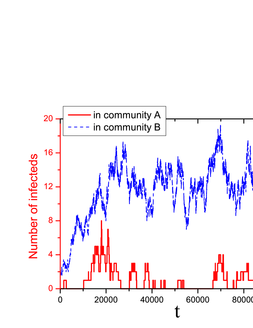
Figure 2: (Colour online) A sample of time series of the number of infected nodes in communities $\mathrm{A}$ (lower, red solid line) and $\mathrm{B}$ (upper, blue dashed line), which are obtained by simulating the model for at least $10^{5}$ time steps after initially only infecting $10$ randomly selected nodes in community $\mathrm{B}$. In the dense community $\mathrm{B}$, the disease persists for the whole time window and the number of infected nodes fluctuates around $60$ after an initial transient regime, whereas the sparse community $\mathrm{A}$ experiences alternations between epidemic outbreaks and extinctions. The parameters are: $N_{\mathrm{A}}=100$, $N_{\mathrm{B}}=200$, $\langle k_{\mathrm{A}}\rangle=4$, $\langle k_{\mathrm{B}}\rangle=12$, $L=10$, $\lambda=0.001$, and $\gamma=0.008$, respectively.

Remarkably, an analogous phenomena have also been observed recently in the study of epidemic spreading in interconnected or coupled networks, with the emergence of a new stable state in which the disease is endemic in one network but neither persists nor dies out in the others [20, 21]. Rather than focusing on the conditions that permit this mixed phase [20, 21], in the present work we probe further the timescales (temporal patterns) of epidemic dynamics in the sparse community. In particular, we examine the time durations of outbreaks and extinctions, and the time interval between two successive inter-community infections, as well as their frequency (probability) distributions. This issue has seldom (if ever) been explored in the literature. However, the direct answer can help us better understand how often infections and extinctions will happen and how long a single outbreak and a single extinction will last in a local community, and thus suggest more effective time-dependent preventive measures.

3 Mean-field Analysis

Denoting by $x_{\mathrm{B}}(t)$ and $y_{\mathrm{B}}(t)$ the fraction of susceptible and infected nodes in the dense community ${\mathrm{B}}$ at time $t$, respectively, one has the normalization condition $x_{\mathrm{B}}(t)+y_{\mathrm{B}}(t)=1$. Since the interconnections between the weakly coupled networks only affect disease spreading in the sparse network [20], by disregarding the infections along the inter-community links we can get the time evolution of the fraction of infected nodes following the MF approach [26]:

$$\frac{\rmd}{\rmd t}y_{\mathrm{B}}(t)=\lambda\langle k_{\mathrm{B}}\rangle x_{\mathrm{B}}(t)y_{\mathrm{B}}(t)-\gamma y_{\mathrm{B}}(t),$$ (1)

where the first term considers the infection of susceptible nodes due to intra-community links, which is proportional to the transmission rate $\lambda$, the average number $\langle k_{\mathrm{B}}\rangle$ of intra-community neighbours per node in community ${\mathrm{B}}$, the density $x_{\mathrm{B}}(t)$ of susceptible nodes, and the probability $y_{\mathrm{B}}(t)$ that a randomly chosen intra-community neighbour is infected, while the second term describes the recovery process of infected nodes, which is proportional to the recovery rate $\gamma$ and the average density $y_{\mathrm{B}}(t)$ of infected nodes. With the assumption $R_{0}^{\mathrm{B}}>1$ and the stationary condition $\frac{d}{dt}y_{\mathrm{B}}(t)=0$, it is straightforward to get the nonzero solution in the steady state,

$$y_{\mathrm{B}}=1-x_{\mathrm{B}}=1-\frac{\gamma}{\lambda\langle k_{\mathrm{B}}\rangle},$$ (2)

which is the epidemic prevalence in community $\mathrm{B}$. In fact, the nontrivial analytical solution to (1) can be written as

$$y_{\mathrm{B}}(t)=\frac{\lambda\langle k_{\mathrm{B}}\rangle-\gamma}{\lambda\langle k_{\mathrm{B}}\rangle-\exp{[-(\lambda\langle k_{\mathrm{B}}\rangle-\gamma)(t-C_{1})]}},$$ (3)

where $C_{1}$ is a constant depending on the initial condition $y_{\mathrm{B}}(0)=\epsilon$. As $t\rightarrow\infty$, (3) again gives rise to the stable fixed point as in (2). The epidemic prevalence $y_{\mathrm{B}}$ can also be translated into the probability that a randomly selected node in community $\mathrm{B}$ becomes infected.

Let $q$ be the probability of disease spreading through the inter-community links from community $\mathrm{B}$ into community $\mathrm{A}$ in one time step. Consider that there are $m$ infected nodes among the $L$ inter-community nodes in community $\mathrm{B}$ at a given time, with a probability ${L\choose m}{y^{m}_{\mathrm{B}}}{(1-y_{\mathrm{B}})}^{L-m}$, and at least one inter-community node in community $\mathrm{A}$ gets infected from the $m$ inter-community links with a probability $[1-(1-\lambda)^{m}]$. Therefore, taking into account all possible numbers ($m=1,2,\ldots,L$) yields

$$q=\sum_{m=1}^{L}{L\choose m}{y^{m}_{\mathrm{B}}}{(1-y_{\mathrm{B}})}^{L-m}[1-(1-\lambda)^{m}].$$ (4)

If one defines $T$ as the time interval between two consecutive inter-community infections, then there is no inter-community infection for a duration of $(T-1)$ time steps until the $T$th time step. As a result, the probability of the time span between two successive inter-community infections being $T$ time steps is

$$P(T)=q(1-q)^{T-1},$$ (5)

and the average time interval between two consecutive inter-community infections is

$$\langle T\rangle=\sum_{T=1}^{\infty}q(1-q)^{T-1}T.$$ (6)

In fact, (4) approximates to

$$q=\sum_{m=1}^{L}{L\choose m}y_{\mathrm{B}}^{m}(1-y_{\mathrm{B}})^{L-m}m\lambda=y_{\mathrm{B}}\lambda L$$ (7)

if one neglects all higher order terms with regard to $\lambda$ in the expression $[1-(1-\lambda)^{m}]$. Furthermore, taking $T$ as continuous in (6) yields

$$\langle T\rangle=\int_{1}^{\infty}q(1-q)^{T-1}T\rmd T=\frac{q[1-\ln(1-q)]}{[\ln(1-q)]^{2}},$$ (8)

which can be simplified to $\langle T\rangle\approx 1/q$ for $q\ll 1$. This approximation treatment is feasible since the value of $\lambda$ is set to be less than $0.01$ and the value of $\lambda L$ set to be up to $0.04$ for all simulations in this context. Therefore the average time interval between two successive outbreaks approximately scales as

$$\langle T\rangle\approx\frac{1}{y_{\mathrm{B}}\lambda L}=\frac{1}{L(\lambda-\gamma/\langle k_{\mathrm{B}}\rangle)}.$$ (9)

As shown in figure 2, community $\mathrm{A}$ is free of disease from the beginning until the epidemic from community $\mathrm{B}$ transmits into this sparse group via the inter-community links — causing an epidemic outbreak. However the infection can only last for a period of time, $T_{i}$, which is defined as the time duration (or span) of the outbreak, since the basic reproductive number is too low ($R_{0}^{\mathrm{A}}<1$) for the disease to persist in community ${\mathrm{A}}$. This means that for a period of $T_{i}$ time steps, the disease exists in community ${\mathrm{A}}$. After that community ${\mathrm{A}}$ is disease-free for a period of time, $T_{s}$, which is defined as the time duration (or span) of the extinction (or health), with all the nodes in the community being susceptible. This disease-free time ends as the next inter-community infection succeeds. In detail, let us assume that the disease initially comes into community $\mathrm{A}$ after $T^{(0)}$ time steps, and after that denote the series of time intervals between consecutive inter-community infections by $T^{(1)},T^{(2)},\ldots$, in sequence. Accordingly, we denote the series of time durations of successive outbreaks by $T^{(1)}_{i},T^{(2)}_{i},\ldots$, and of successive extinctions by $T^{(1)}_{s},T^{(2)}_{s},\ldots$, see figure 3 for an illustration.

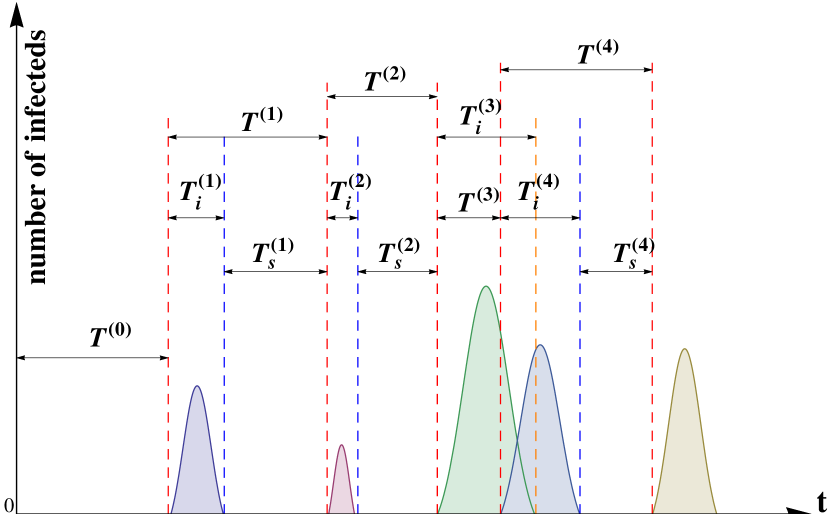
Figure 3: (Colour online) Diagrammatic illustration for the relationship between the three time durations: $T^{(j)}$, $T_{i}^{(j)}$, and $T_{s}^{(j)}$, with the superscript $j$ denoting the $j$th event of inter-community infection [excluding the first period $T^{(0)}$], temporary epidemic outbreak and disease extinction in community $\mathrm{A}$, respectively. For theoretical analysis, we define an artificial (negative) time duration of disease extinction [e.g., here, $T_{s}^{(3)}=T^{(3)}-T_{i}^{(3)}$] for the case of overlaps between two successive epidemic outbreaks. Note that the curves on top of the coloured areas do not represent the real number of infected individuals, this is just for illustration.

It is complicated to derive theoretically the time spans $T_{i}$ and $T_{s}$ due to the potential effects of inter-community infections and the overlaps between successive epidemic outbreaks, which occur when a new inter-community infection emerges before the old disease dies out. However, there is a definite relationship between the values of these three time spans. As seen in figure 3, if two successive outbreaks do not overlap, then the time interval between these two infections is equal to the sum of the time duration of the former outbreak and the disease-free period before the latter outbreak. Mathematically, that is

$$T=T_{i}+T_{s}\quad\quad\mathrm{if}\quad T>T_{i}.$$ (10)

For example, from figure 3 one can obtain $T^{(1)}=T_{i}^{(1)}+T_{s}^{(1)}$, $T^{(2)}=T_{i}^{(2)}+T_{s}^{(2)}$, and $T^{(4)}=T_{i}^{(4)}+T_{s}^{(4)}$, but can not get a time duration of health during the time interval of $T^{(3)}$, since $T^{(3)}<T_{i}^{(3)}$. For analysis in theory, we specifically define a virtual (negative) time span of health as $T_{s}^{(j)}=T^{(j)}-T_{i}^{(j)}$ for the case of $T^{(j)}<T_{i}^{(j)}$ associated to the corresponding overlap. Such a treatment allows us to use the relationship given in (10) in the presence of overlaps between consecutive outbreaks.

Once a node in community $\mathrm{A}$ gets infected by an inter-community infection, it will trigger a temporal dynamical process in its local community before a subsequent inter-community infection occurs. Therefore, by omitting the effects of inter-community transmissions, one can write the evolution equation for $y_{\mathrm{A}}(t)$, the density of infected nodes in community $\mathrm{A}$, similar to (1), as

$$\frac{d}{dt}y_{\mathrm{A}}(t)=(\lambda\langle k_{\mathrm{A}}\rangle-\gamma)y_{\mathrm{A}}(t)-\lambda\langle k_{\mathrm{A}}\rangle y^{2}_{\mathrm{A}}(t).$$ (11)

Here, the second-order term arises from the normalization condition where $x_{\mathrm{A}}(t)=1-y_{\mathrm{A}}(t)$ has been eliminated from the equation. One can also work out the nontrivial solution to (11) which resembles (3). Nonetheless, this can not be used to evaluate the time duration of an outbreak because this solution contains a constant closely related to the initial fraction of infected individuals $y_{\mathrm{A}}(0)$, which is stochastic. Since $\frac{d}{dt}y_{\mathrm{A}}(t)<0$ for $R_{0}^{\mathrm{A}}<1$, the density of infected individuals decreases with time and is difficult to reach a relatively high level. Therefore, we neglect the second-order term with regard to $y_{\mathrm{A}}(t)$ in (11) and obtain an approximate solution

$$y_{\mathrm{A}}(t)\approx y_{\mathrm{A}}(0)\exp{[-(\gamma-\lambda\langle k_{\mathrm{A}}\rangle)t]}.$$ (12)

We estimate the time period of the outbreak by applying the concept of half-life ($t_{1/2}$) [28], generally defined as the time required for a quantity to diminish to half its value as measured at the beginning of the time period, which is typically used to describe a quantity that follows an exponential decay. Setting $y_{\mathrm{A}}(t)/y_{\mathrm{A}}(0)=1/2$, one gets the half-life

$$t_{1/2}=\frac{\ln 2}{\gamma-\lambda\langle k_{\mathrm{A}}\rangle}$$ (13)

for the density of infected individuals. After $n$ half-lives, the density drops from $y_{\mathrm{A}}(0)$ to $y_{\mathrm{A}}(0)/{2^{n}}$. In the present work we use the time, which is required for the number of infected nodes $I^{\mathrm{A}}_{t}=y_{\mathrm{A}}(t)N_{\mathrm{A}}$ to drop from the initial value $I^{\mathrm{A}}_{0}=y_{\mathrm{A}}(0)N_{\mathrm{A}}$ to $\frac{1}{2}$ (where the disease is close to extinction), to estimate the time duration $T_{i}$ of the outbreak [Strictly this accumulation of half-lives is not exactly the time span $T_{i}$ for the entire outbreak; this approximation, however, matches the qualitative behaviour of $T_{i}$ and can provide a similar scaling shape (if not the size), as shown in section 4.]. Thus, letting $I^{\mathrm{A}}_{0}/{2^{n}}=\frac{1}{2}$ gives rise to $n=1+\log_{2}{I^{\mathrm{A}}_{0}}$. Consequently, the time duration $T_{i}$ is dependent on the initial number of infected nodes in community $\mathrm{A}$ in such a way that $T_{i}(I^{\mathrm{A}}_{0})=nt_{1/2}=(1+\log_{2}{I^{\mathrm{A}}_{0}})t_{1/2}$. Since there are a number $L$ of inter-community links between the two communities, all possible numbers of infected nodes at the beginning of the outbreak period are $I^{\mathrm{A}}_{0}=1,2,\ldots,L$ as these $I^{\mathrm{A}}_{0}$ inter-community links pass the disease simultaneously with the probability

$$P(I^{\mathrm{A}}_{0})=\sum_{\ell=I^{\mathrm{A}}_{0}}^{L}{L\choose\ell}y_{\mathrm{B}}^{\ell}(1-y_{\mathrm{B}})^{L-\ell}{\ell\choose I^{\mathrm{A}}_{0}}\lambda^{I^{\mathrm{A}}_{0}}(1-\lambda)^{\ell-I^{\mathrm{A}}_{0}}.$$ (14)

By definition it is clear that $\sum_{I^{\mathrm{A}}_{0}=1}^{L}P(I^{\mathrm{A}}_{0})=q$, whereby we normalize $P(I^{\mathrm{A}}_{0})$ to obtain the average time duration of an epidemic outbreak as follows:

$$\langle T_{i}\rangle=\frac{1}{q}\sum_{I^{\mathrm{A}}_{0}=1}^{L}T_{i}{(I^{\mathrm{A}}_{0})}P(I^{\mathrm{A}}_{0})=\frac{\ln 2}{q(\gamma-\lambda\langle k_{\mathrm{A}}\rangle)}\sum_{I^{\mathrm{A}}_{0}=1}^{L}(1+\log_{2}{I^{\mathrm{A}}_{0}})P(I^{\mathrm{A}}_{0}).$$ (15)

For simplicity in theory, we estimate the average timescale of a single disease-free phase as

$$\langle T_{s}\rangle=\langle T\rangle-\langle T_{i}\rangle,$$ (16)

using the expression in (10), regardless of whether there are overlaps between successive outbreaks.

Now, we analyze the frequency distributions $P(T)$ and $P(T_{i})$ of the timescales $T$ and $T_{i}$, respectively. In accordance with (5), one has

$$P(T)\approx q\exp{(-qT)}$$ (17)

for a negligibly small $q$, since

$$(1-q)^{T}=\exp{(-qT)}-\frac{T}{2}q^{2}+o(q^{2}).$$ (18)

The approximate solution (12) implies that an epidemic outbreak’s probability of still existing at a time $t$ after its first appearance is $\exp{[-(\gamma-\lambda\langle k_{\mathrm{A}}\rangle)t]}$. Since the probability of disappearing during the time interval $[t,t+\rmd t]$ is $(\gamma-\lambda\langle k_{\mathrm{A}}\rangle)\exp{[-(\gamma-\lambda\langle k_{\mathrm{A}}\rangle)t]}\rmd t$, we arrive at an exponential probability distribution

$$P(T_{i})=(\gamma-\lambda\langle k_{\mathrm{A}}\rangle)\exp{[-(\gamma-\lambda\langle k_{\mathrm{A}}\rangle)T_{i}]}.$$ (19)

Figure 4: (Colour online) The average time interval $\langle T\rangle$ between two successive inter-community infections in community $\mathrm{A}$ as a function of: the number $L$ of inter-community links (with $\langle k_{\mathrm{A}}\rangle=4$, $\langle k_{\mathrm{B}}\rangle=12$, $\lambda=0.001$, and $\gamma=0.008$) (a); the average node degree $\langle k_{\mathrm{B}}\rangle$ within community $\mathrm{B}$ (with $L=4$, $\langle k_{\mathrm{A}}\rangle=4$, $\lambda=0.001$, and $\gamma=0.008$) (b); the average node degree $\langle k_{\mathrm{A}}\rangle$ within community $\mathrm{A}$ (with $L=20$, $\langle k_{\mathrm{B}}\rangle=40$, $\lambda=0.01$, and $\gamma=0.0005$) (c); the transmission rate $\lambda$ (with $L=4$, $\langle k_{\mathrm{A}}\rangle=4$, $\langle k_{\mathrm{B}}\rangle=20$, and $\gamma=0.04$) (d); and the recovery rate $\gamma$ (with $L=4$, $\langle k_{\mathrm{A}}\rangle=4$, $\langle k_{\mathrm{B}}\rangle=24$, and $\lambda=0.001$) (e), respectively. The log-log plot of $\langle T\rangle$ in the inset of (a) exhibits a power law $\langle T\rangle\propto L^{-1}$, which is consistent with (9). The black circles represent the simulation results and the red lines denote the theoretical calculations by (6).

Figure 5: (Colour online) The average time period $\langle T_{i}\rangle$ of epidemic outbreak as a function of: the number $L$ of inter-community links (with $\langle k_{\mathrm{A}}\rangle=4$, $\langle k_{\mathrm{B}}\rangle=12$, $\lambda=0.001$, and $\gamma=0.008$) (a); the average node degree $\langle k_{\mathrm{B}}\rangle$ within community $\mathrm{B}$ (with $L=4$, $\langle k_{\mathrm{A}}\rangle=4$, $\lambda=0.001$, and $\gamma=0.008$) (b); the average node degree $\langle k_{\mathrm{A}}\rangle$ within community $\mathrm{A}$ (with $L=20$, $\langle k_{\mathrm{B}}\rangle=40$, $\lambda=0.01$, and $\gamma=0.0005$) (c); the transmission rate $\lambda$ (with $L=4$, $\langle k_{\mathrm{A}}\rangle=4$, $\langle k_{\mathrm{B}}\rangle=20$, and $\gamma=0.04$) (d); and the recovery rate $\gamma$ (with $L=4$, $\langle k_{\mathrm{A}}\rangle=4$, $\langle k_{\mathrm{B}}\rangle=24$, and $\lambda=0.001$) (e), respectively. The black circles represent the simulation results and the solid lines denote the theoretical results obtained by (15). The blue error bars shown in the panels (a) and (b) are the standard deviation.

Figure 6: (Colour online) The average time period $\langle T_{s}\rangle$ of an extinction as a function of: the number $L$ of inter-community links (with $\langle k_{\mathrm{A}}\rangle=4$, $\langle k_{\mathrm{B}}\rangle=12$, $\lambda=0.001$, and $\gamma=0.008$) (a); the average node degree $\langle k_{\mathrm{B}}\rangle$ within community $\mathrm{B}$ (with $L=4$, $\langle k_{\mathrm{A}}\rangle=4$, $\lambda=0.001$, and $\gamma=0.008$) (b); the average node degree $\langle k_{\mathrm{A}}\rangle$ within community $\mathrm{A}$ (with $L=20$, $\langle k_{\mathrm{B}}\rangle=40$, $\lambda=0.01$, and $\gamma=0.0005$) (c); the transmission rate $\lambda$ (with $L=4$, $\langle k_{\mathrm{A}}\rangle=4$, $\langle k_{\mathrm{B}}\rangle=20$, and $\gamma=0.04$) (d); and the recovery rate $\gamma$ (with $L=4$, $\langle k_{\mathrm{A}}\rangle=4$, $\langle k_{\mathrm{B}}\rangle=24$, and $\lambda=0.001$) (e), respectively. The black circles represent the simulation results and the solid lines denote the theoretical results obtained by (16).

Figure 7: (Colour online) Red squares represent the relative Errors $\Delta T_{s}$ [defined by (20)] of the average disease-free time period $\langle T_{s}\rangle$, of which the theoretical and numerical results are correspondingly demonstrated in figure 6. Blue circles denote the probability $P(T>T_{i})$ of no overlaps of epidemic outbreaks. All the results show that the fewer overlaps between successive outbreaks, the more accurate theoretical prediction.

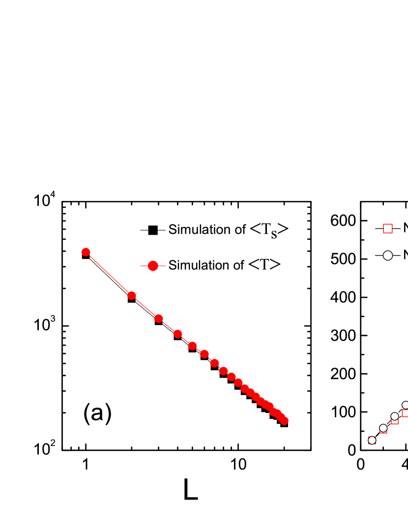
Figure 8: (Colour online) Comparison of the simulation results (a) as well as the numbers of events (b) between $\langle T\rangle$ (represented by circles) and $\langle T_{s}\rangle$ (represented by squares) as the number of inter-community links $L$ varies. The parameter values are the same as in figure 4(a).

Figure 9: (Colour online) Frequency distributions of: $T$, the time interval between successive inter-community infections (a); $T_{i}$, the time duration of epidemic outbreak (b); and $T_{s}$, the time period of disease-free (c). The simulation results shown in the histogram are obtained after statistically counting the number of events in each bin of width of $200$ time steps, with the solid circles representing the counts of bin centers, while the red lines in (a) and (b) represent the theoretical results obtained by integrating Eqs. (17) and (19) over each bin respectively. Parameter values are $L=10$, $\langle k_{\mathrm{A}}\rangle=4$, $\langle k_{\mathrm{B}}\rangle$, $\lambda=0.001$, and $\gamma=0.008$. The total numbers of events for $T$, $T_{i}$, and $T_{s}$ are $13812$, $8439$, and $8514$, respectively.

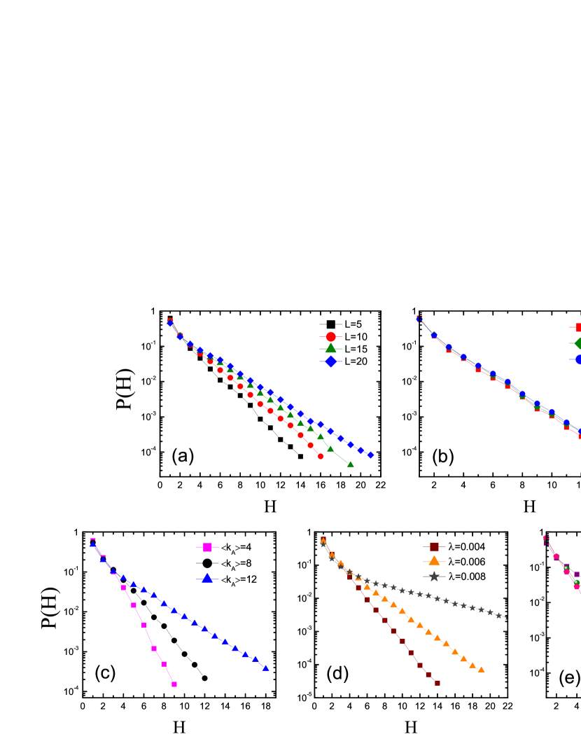
Figure 10: (Colour online) Probability distribution $P(H)$ of the height of epidemic outbreaks: for various values of $L$: 5, 10, 15, 20 (from bottom to top), with $\langle k_{\mathrm{A}}\rangle=4$, $\langle k_{\mathrm{B}}\rangle=12$, $\lambda=0.001$, and $\gamma=0.008$ (a); for various values of $\langle k_{\mathrm{B}}\rangle$: 12, 18, 24 (from bottom to top), with $L=4$, $\langle k_{\mathrm{A}}\rangle=4$, $\lambda=0.001$, and $\gamma=0.008$ (b); for different values of $\langle k_{\mathrm{A}}\rangle$: 4, 8, 12 (from bottom to top), with $L=20$, $\langle k_{\mathrm{B}}\rangle=40$, $\lambda=0.01$, and $\gamma=0.0005$ (c); for various values of $\lambda$: 0.004, 0.006, 0.008 (from bottom to top), with $L=4$, $\langle k_{\mathrm{A}}\rangle=4$, $\langle k_{\mathrm{B}}\rangle=20$, and $\gamma=0.04$ (d); and for distinct values of $\gamma$: 0.006, 0.009, 0.012 (from top to bottom), with $L=4$, $\langle k_{\mathrm{A}}\rangle=4$, $\langle k_{\mathrm{B}}\rangle=24$, and $\lambda=0.001$ (e), respectively.

4 Results and discussions

4.1 Average timescales

We test theoretical predictions of the proviso section with computational simulations of the epidemiological model over a random network with community structure. We consider two ER communities $\mathrm{A}$ and $\mathrm{B}$ with $N_{\mathrm{A}}=10^{3}$ and $N_{\mathrm{B}}=2\times 10^{3}$ nodes, respectively. We start the simulation with no infection in community $\mathrm{A}$ and a fraction $\epsilon=0.5\%$ of infected nodes in community $\mathrm{B}$, and then let the epidemic spreading go through $10^{5}$ time steps for each realization. By recording the starting time of each epidemic outbreak in community $\mathrm{A}$ arising from the inter-community infections, we measure the time interval $T$ between two consecutive outbreaks. We compute the time period, during which at least one infected node exists in community $\mathrm{A}$, as the time duration $T_{i}$ of an epidemic outbreak, and take the time period, during which there is no disease in this community, as the disease-free time duration $T_{s}$ of an extinction of disease. Note that the time periods $T_{i}$ and $T_{s}$ calculated in simulations are different from their theoretical estimates as long as there are overlaps between epidemic outbreaks. See figure 3 for example, in case of an overlap between the third and the fourth outbreaks, we numerically record one single epidemic outbreak with a time period $[T^{(3)}+T_{i}^{(4)}]$ rather than two individual outbreaks with time periods $T_{i}^{(3)}$ and $T_{i}^{(4)}$, respectively. In addition, the numerical $T_{s}$ considers only the positive time periods of extinction while disregarding the overlaps of epidemic outbreaks.

To study the dependence of the average timescales on the network structure and the transmission parameters, we calculate $\langle T\rangle$, $\langle T_{i}\rangle$, and $\langle T_{s}\rangle$ by varying each of the values of $L$, $\langle k_{\mathrm{A}}\rangle$, $\langle k_{\mathrm{B}}\rangle$, $\lambda$, and $\gamma$ in such a proper range that ensures $R_{0}^{\mathrm{A}}<1$, $R_{0}^{\mathrm{B}}>1$, and $R_{0}^{\mathrm{Net}}>1$. All the simulation results shown in the following figures are calculated averaging over at least $20$ different initial network configurations, each performed on $50$ realizations of the epidemiological model.

Figure 4 shows the average time interval $\langle T\rangle$ between two successive epidemic outbreaks in community $\mathrm{A}$ as a function of the number $L$ of inter-community links [see figure 4(a)], the average intra-community node degree $\langle k_{\mathrm{B}}\rangle$ of community $\mathrm{B}$ [see figure 4(b)], the average intra-community node degree $\langle k_{\mathrm{A}}\rangle$ of community $\mathrm{A}$ [see figure 4(c)], the transmission rate $\lambda$ [see figure 4(d)], and the recovery rate $\gamma$ [see figure 4(e)], respectively. On one hand, $\langle T\rangle$ decreases as $L$, $\langle k_{\mathrm{B}}\rangle$, and $\lambda$ increase. On the other hand, $\langle T\rangle$ increases with $\gamma$, while keeping unchanged for varying values of $\langle k_{\mathrm{A}}\rangle$. The more the inter-community links (or the denser the community $\mathrm{B}$ or the larger the infection rate or the smaller the recovery rate), the easier the inter-community infections (i.e., the easier for the disease to spread from community $\mathrm{B}$ into community $\mathrm{A}$), which suggests a shorter time period between two successive epidemic outbreaks. On the contrary, the property $\langle k_{\mathrm{A}}\rangle$ inherent in the sparse community $\mathrm{A}$ has no contribution to the inter-community infections which originate from the dense community $\mathrm{B}$. Such behaivour of $\langle T\rangle$ related to each of these parameters, including the linearity shown in the log-log plot in the inset of figure 4(a), confirms the MF analysis (9) in section 3. All the theoretical results by the MF approach are smaller than the simulations, since the MF approximation in (1) has ignored the higher-order terms of $y_{\mathrm{B}}$, which leads to an overestimate for $y_{\mathrm{B}}$, and thus causes $\langle T\rangle$ to be underestimated according to (7) and (9).

Figure 5 shows the mean time period $\langle T_{i}\rangle$ of an epidemic outbreak in community $\mathrm{A}$ versus parameters $L$, $\langle k_{\mathrm{B}}\rangle$, $\langle k_{\mathrm{A}}\rangle$, $\lambda$, and $\gamma$, respectively. The theoretical prediction of $\langle T_{i}\rangle$ remains almost unchanged with the increase of $L$, whereas the simulation result shows a monotonous increase. The reason for this is that the theoretical prediction is based on the half-life calculation (13) and only measures part of the real period of the outbreak and also neglects the effects of inter-community infections during the period of an epidemic outbreak in the sparse community. In view of the fact that the more the links between the two communities, the easier for the inter-community transmission to happen. Thus, one would expect a larger probability of overlaps between successive outbreaks [see figure 7(a)], which causes numerical counting of $\langle T_{i}\rangle$ to be more likely to exceed the theoretical prediction. Therefore, it is hard to predict the average time period of an epidemic outbreak if there are a large number of inter-community links. A similar explanation can also be made for the difference between the analysis and simulation in figure 5(b), where the simulation results grow slightly with the increase of $\langle k_{\mathrm{B}}\rangle$, whereas the analytical results are almost unchanged. The higher density of connections inside community $\mathrm{B}$ leads to a larger fraction of infected node in this community in the steady state, which suggests a greater probability of overlaps between epidemic outbreaks [see figure 7(b)]. However, the inter-community transmissions are heavily restricted since the number of inter-community links is set to $L=4$, which can explain why the simulation results of $\langle T_{i}\rangle$ increases slowly compared to figure 5(a).

Moreover, we find from figure 5(c) and figure 5(d) that both the analytical predictions and the simulation results of $\langle T_{i}\rangle$ rise with the increase of $\langle k_{\mathrm{A}}\rangle$ and $\lambda$, separately. For smaller values of $\langle k_{\mathrm{A}}\rangle$ and $\lambda$, the predictions are smaller than the simulations. This is due to the increase of $\langle k_{\mathrm{A}}\rangle$ and $\lambda$ promoting the disease spread and thus enhancing the possibility of overlapping outbreaks, as seen in figure 7(c) and figure 7(d). However, after the values of $\langle k_{\mathrm{A}}\rangle$ and $\lambda$ increase to a certain point, we see the reverse case, i.e., the theoretical results are larger than the numerical results. It stems from the simplification of (11) by discarding the second order term in $y_{\mathrm{A}}$. This approximation treatment generally produces relatively tiny errors if the second order term is far less than the first order term with respect to $y_{\mathrm{A}}$. On the other hand, when the values of $\langle k_{\mathrm{A}}\rangle$ and $\lambda$ become large enough so that $(\gamma-\lambda\langle k_{\mathrm{A}}\rangle)$ approaches zero and hence the first term closes to the second term in (11) even for a very low level of $y_{\mathrm{A}}$. In this case, neglecting the higher order term in $y_{\mathrm{A}}$ will considerably underestimate the decaying speed of $y_{\mathrm{A}}$ and hence greatly overestimate the outbreak duration. In addition, as shown in figure 5(e), both analytically and numerically the average time period of $\langle T_{i}\rangle$ decreases with the recovery rate $\gamma$. With a higher recovery rate, the infected nodes will recover faster before they are able to spread the disease to susceptible nodes, therefore the epidemic outbreak will last for a shorter time. The theoretical prediction is smaller than the simulation result because the half-life approximation only captures part of the real time period of $\langle T_{i}\rangle$.

Figure 6 displays the average time period $\langle T_{s}\rangle$ of an extinction (i.e., a disease-free period) versus $L$ [see figure 6(a)]; $\langle k_{\mathrm{B}}\rangle$ [see figure 6(b)]; $\langle k_{\mathrm{A}}\rangle$ [see figure 6(c)]; $\lambda$ [see figure 6(d)]; and $\gamma$ [see figure 6(e)], respectively. For all parameters, the theoretical predictions given by (16) are smaller than the simulation results. This is to be expected since (16) covers both the positive part $\sum_{T>T_{i}}(T-T_{i})P(T-T_{i})$ and the negative part $\sum_{T<T_{i}}(T-T_{i})P(T-T_{i})$ whereas the simulation counting considers only the positive part by ignoring those situations which include an overlap between successive epidemic outbreaks. The negative part accounts for a larger proportion if the probability of overlapping outbreaks is larger, which will greatly reduce the accuracy of the theoretical estimates of $\langle T_{s}\rangle$.

4.2 Relative errors of $\langle T_{s}\rangle$

Based on the above discussion, the deviation between the theoretical and simulation results of $\langle T_{s}\rangle$ decreases with the probability $P(T>T_{i})$ that the time interval between two successive outbreaks is larger than the time duration of the former outbreak (with $1-P(T>T_{i})$ being actually the probability of overlapping outbreaks). To confirm this, we plot in figure 7 the relative error $\Delta T_{s}$ of the mean time duration of disease extinction $\langle T_{s}\rangle$, which is defined as

$$\Delta T_{s}=\frac{\big{|}{\langle T_{s}\rangle}_{\mathrm{simulation}}-{\langle T_{s}\rangle}_{\mathrm{theory}}\big{|}}{{\langle T_{s}\rangle}_{\mathrm{simulation}}}$$ (20)

and can help examine the accuracy of the theoretical prediction of $\langle T_{s}\rangle$. A smaller $\Delta T_{s}$ denotes a more accurate prediction of $\langle T_{s}\rangle$. As demonstrated in figure 7, the accuracy of the theoretical estimates of $\langle T_{s}\rangle$ decreases with the increase of $L$, $\langle k_{\mathrm{B}}\rangle$, $\langle k_{\mathrm{A}}\rangle$, and $\lambda$, respectively. It is attributed to a larger number of inter-community links (or a larger average node degree within each community or a larger transmission rate) leading to a larger likelihood of overlapping outbreaks. In particular, for large values of $\langle k_{\mathrm{A}}\rangle$ [see figure 7(c)] and $\lambda$ [see figure 7(d)] the accuracy of $\langle T_{s}\rangle$ becomes worse. Since $\langle k_{\mathrm{A}}\rangle$ or $\lambda$ is large enough, the theory of $\langle T_{i}\rangle$ is much larger than its simulation, causing $\langle T\rangle-\langle T_{i}\rangle$ to decline rapidly and become negative. Conversely, the theoretical prediction of $\langle T_{s}\rangle$ is more accurate for a larger value of $\gamma$, as shown in figure 7(e).

In addition, we observe an interesting fact that for all the parameters $L$, $\langle k_{\mathrm{B}}\rangle$, $\langle k_{\mathrm{A}}\rangle$, $\lambda$, and $\gamma$, the simulation results of $\langle T_{s}\rangle$ are very close to those of $\langle T\rangle$. As an example we demonstrate a comparison between the simulation results of $\langle T_{s}\rangle$ and $\langle T\rangle$ as $L$ varies in figure 8(a), and the numbers of events for both the inter-community infections and disease extinctions are also reported in figure 8(b). For a smaller value of $L$, the numbers of both events are closer, meaning that the frequency of outbreak overlaps is smaller, thus the difference between $\langle T\rangle$ and $\langle T_{s}\rangle$ approaches to $\langle T_{i}\rangle$, which is significantly smaller compared to $\langle T\rangle$ at the small point of $L$. On the other hand, for a larger $L$, the more frequent overlaps of outbreaks offset the difference between $\langle T\rangle$ and $\langle T_{s}\rangle$ by counting the small $T$ that satisfies $T<T_{i}$. So, the simulation results of $T$ and $\langle T_{s}\rangle$ are close for the whole range of $L$. Similar results are also found in the simulations for the other parameters.

4.3 Distributions of the epidemic timescales

It is clear from figure 9(a) that both the theoretical and numerical results of $P(T)$ follow an exponential distribution. Note that the simulation results have been counted for the frequency distribution of $T$ and plotted in a histogram with an equal bin of width $200$ time steps. The theoretical results depicted by the red line are obtained after multiplying the integral of (17) over each bin by the total event count ($13812$ in this example). Apparently, the theoretical results decay faster, with a steeper slope ($-q$), than the simulation. As mentioned before, the MF approximation in (1) overestimates the value of $y_{\mathrm{B}}$ and hence, according to (7), the theoretical value of $q$ is larger than the numerical one. As shown in figure 9(b), both the theory and the simulation exhibit an exponential frequency distribution of the time duration $T_{i}$ of an epidemic outbreak. Analogous to figure 9(a), the simulation results in figure 9(b) are plotted as a histogram, where the theoretical points present on the red line are given by integrating (19) over each bin of width $200$ time steps and then multiplying the outcomes by the total event count — $8439$. For small values of $T_{i}$ [see the range $0<T_{i}<400$ in figure 9(b)], the simulation results of $P(T_{i})$ decrease faster than the analytical prediction by (19) because the approximation used in (12) neglects the second order term with regard to $y_{\mathrm{A}}$ in (11) and thus underestimates the decaying speed compared with the simulation results. On the other hand, for larger values of $T_{i}$, the simulation results decay slower than the theory, because the frequent overlaps between consecutive epidemic outbreaks help extend the outbreak duration in the simulation computing. Since both $P(T)$ and $P(T_{i})$ are exponential, the relationship given by (10) allows us to expect an exponential frequency distribution for $T_{s}$, which is confirmed by the simulation results shown in the histogram of figure 9(c).

4.4 Distributions of the peak heights

Inspired by the intermittent occurrences of epidemic outbreaks in the sparse community $\mathrm{A}$, we further numerically investigate the probability distribution $P(H)$ of the “height” of an epidemic outbreak $H$, which is defined as the maximal number of infected nodes during the outbreak. The simulation results of $P(H)$ for various values of each of the parameters $L$, $k_{\mathrm{B}}$, $k_{\mathrm{A}}$, $\lambda$, and $\gamma$ are shown in figure 10, and all decay exponentially. This results from that the frequency distribution $P(T_{i})$ of time duration of an outbreak follows an exponential decay, and, the longer the outbreak duration $T_{i}$ the larger the probability that the outbreak has a large height $H$. Figure 10(a) reveals that the more the inter-community links, the more possible for the epidemic outbreak to climb to a large height. According to the simulation results in figure 5(a), a larger $L$ suggests a longer time duration $\langle T_{i}\rangle$ of an outbreak since it is more likely to cause overlaps between successive outbreaks, thus it is easier to obtain a large $H$. From figure 10(b) we observe that for a fixed value of $H$, the value of $P(H)$ increases very slightly as $k_{\mathrm{B}}$ increases from $12$ to $18$ and further to $24$. It arises from the increment of $k_{\mathrm{B}}$ resulting in a slight growth of $\langle T_{i}\rangle$ in simulations since the relative small number ($L=4$) of inter-community links restricts the inter-community infections, as explained for figure 5(b). Based on (19), we expect a higher frequency $P(T_{i})$ for larger values of $\langle k_{\mathrm{A}}\rangle$ and $\lambda$ or for a smaller value of $\gamma$. Thus, one can expect an increase of $P(H)$ with the increase of $\langle k_{\mathrm{A}}\rangle$ and $\lambda$ or with the decrease of $\gamma$, both of which is supported by simulation results [see figure 10(c-e)].

5 Conclusion

We have studied the SIS model in a random network composed of a dense community $\mathrm{B}$ and a sparse community $\mathrm{A}$, where the disease persists throughout the dense community while in the sparse community it alternates between temporary epidemic outbreaks and extinctions. The model is particularly relevant for disease transmission from a reservoir population and intermittent outbreak in a secondary group, as is the case with many zoonotic or emerging infectious diseases. We have developed a theoretical framework and performed extensive computational simulations to understand the interesting features of the epidemic dynamics in the sparse community. In particular, we have explored the expected values for the time durations of outbreak and extinction, the time interval between two successive outbreaks, and their frequency distributions. The results demonstrated how these timescales rely on the parameters including the number $L$ of inter-community links, the average node degree $\langle k_{\mathrm{B}}\rangle$ within community $\mathrm{B}$ and $\langle k_{\mathrm{A}}\rangle$ within community $\mathrm{A}$, the transmission rate $\lambda$, and the recovery rate $\gamma$. The theoretical results are in good agreement with simulations except when there are too frequent overlaps between successive epidemic outbreaks, since such overlaps extend the time duration of outbreak and make the simulation computing deviate from the theory. We have also found an exponential decay for the frequency distributions of these timescales, as well as for the frequency distribution of the maximal number of infections during an epidemic outbreak. All these results may provide helpful insights for understanding the temporal patterns of an epidemic in a local community and lead to draw up effective time-based preventive strategies. For example, the temporal pattern of inter-community infections may suggests we implement a periodic vaccination plan on the inter-community nodes in the sparse community after each time period $\langle T\rangle$. More effectively, according to the exponential distribution of the time interval $T$ between successive inter-community infections, we may also consider exponentially distributed vaccination forces $\nu\propto exp(-qT)$ on the inter-community nodes in the sparse community, with regard to the waiting time $T$ since the first appearance of infection in the dense community.

This paper only considers the simplest network topology, i.e., the ER random graph, which is an important example of homogeneous networks. Therefore, it is of great interest to extend the present work to heterogeneous networks, which needs a deeper study since the heterogeneities in node degrees make it more complicated to make an accurate prediction for the epidemic timescales. It is worth notice that the MF theory provides a good approximation for the prediction of the average timescale of $T$ and its distribution $P(T)$, which largely benefits from the fact that in the dense ER community, every node has a high degree and so do the nearest neighbours of any given node, where the MF theory generally yield good approximations to the underlying dynamical process [29]. However, as shown in the present work, the ignorance of higher-order correlations with respect to infectious density in the MF equation can lead to a small deviation from the simulations.

References

References

- [1] Albert R and Barabási A L 2002 Rev. Mod. Phys. 74 47
- [2] Newman M E J 2010 Networks: An Introduction (New York: Oxford University Press)
- [3] Pastor-Satorras R and Vespignani A 2004 Evolution and Structure of the Internet (New York: Cambridge University Press)
- [4] Barrat A, Barthélemy M and Vespignani A 2008 Dynamical Processes on Complex Networks (New York: Cambridge University Press)
- [5] Girvan M and Newman M E J 2002 Proc. Natl. Acad. Sci. USA 99 7821
- [6] Radicchi F, Castellano C, Cecconi F, Loreto V and Parisi D 2004 Proc. Natl. Acad. Sci. USA 101 2658
- [7] Newman M E J 2006 Proc. Natl. Acad. Sci. USA 103 8577
- [8] Leicht E A and Newman M E J 2008 Phys. Rev. Lett. 100 118703
- [9] Porter M A, Onnela J-P and Mucha P J 2009 Not. Am. Math. Soc. 56 1082
- [10] Fortunato S 2010 Phys. Rep. 486 75
- [11] Liu Z and Hu B 2005 Europhys. Lett. 72 315
- [12] Huang L, Park K and Lai Y C 2006 Phys. Rev. E 73 035103(R)
- [13] Salathé M and Jones J H 2010 PLoS Comput. Biol. 6 e1000736
- [14] Kitchovitch S and Liò P 2011 PLoS ONE 6 e22220
- [15] Lentz H H K, Selhorst T and Sokolov I M 2012 Phys. Rev. E 85 066111
- [16] Collizza V, Pastor-Satorras R and Vespignani A 2007 Nature Phys. 3 276
- [17] Liu S Y, Baronchelli A and Perra N 2013 Phys. Rev. E 87 032805
- [18] Saumell-Mendiola A, Serrano M Á and Boguñá M 2012 Phys. Rev. E 86 026106
- [19] Mills H L, Ganesh A and Colijin C 2013 J. Theor. Biol. 320 47
- [20] Dickison M, Havlin S and Stanley H E 2012 Phys. Rev. E 85 066109
- [21] Shai S and Dobson S 2013 Phys. Rev. E 87 042812
- [22] Anderson R M and May R M 1991 Infectious Diseases of Humans: Dynamics and Control (Oxford: Oxford University Press)
- [23] Greger M 2007 Crit. Rev. Microbiol. 33 243
- [24] Berns K I et al. 2012 Nature 482 153
- [25] Webby R J and Webster R G 2003 Science 302, 1519
- [26] Pastor-Satorras R and Vespignani A 2001 Phys. Rev. E 63 066117
- [27] Erdös P and Rényi A 1960 Publ. Math. Inst. Hung. Acad. Sci. 5 17
- [28] Refer to http://en.wikipedia.org/wiki/Half-life for the information of half-life.
- [29] Gleeson J P, Melnik S, Ward J A, Porter M A and Mucha P J 2012 Phys. Rev. E 85 026106