Blow-up regimes in the $\mathcal{PT}$- and the $\mathcal{AC}$-dimer

Abstract

In the actively coupled ($\mathcal{AC}$) pair of waveguides, the growth of small perturbations is saturated by the focussing nonlinearity that couples the linearly growing to the linearly damped mode. On the other hand, in the $\mathcal{PT}$-symmetric coupler, the focussing nonlinearity promotes the blowup of stationary light beams. The purpose of this study is to compare the nonlinear dynamics and explain the opposite effect of the same nonlinearity in the two systems. We show that while the blowup regimes are stable in the $\mathcal{PT}$-symmetric pair of waveguides, they are unstable and hence cannot be observed in the $\mathcal{AC}$-dimer.

I Introduction

The current growth of interest in the $\mathcal{PT}$-symmetric photonic systems with gain and loss PT_breaking ; SXK ; RKEC ; Musslimani ; Zheng ; Longhi ; Guo ; Ramezani ; Rueter ; Recent_PT ; BSSDK is motivated by the unusual phenomenology associated with these systems. Optical structures composed of coupled active and lossy elements exhibit symmetry-breaking phase transitions SXK ; Rueter ; PT_breaking , unconventional beam refraction Musslimani ; Zheng , nonreciprocity Longhi ; Rueter , loss-induced transparency Guo , conical diffraction Ramezani , and beam breathing SXK ; Musslimani ; Rueter ; BSSDK . The nonlinear effects in such systems can be utilised for an efficient control of light, including all-optical low-threshold switching RKEC ; SXK and unidirectional invisibility SXK ; RKEC . One of the two objects considered in the present paper is the simplest $\mathcal{PT}$-symmetric optical system consisting of a single waveguide with loss coupled to a waveguide with an equal amount of gain.

The gain-loss systems — and in particular the $\mathcal{PT}$-symmetric coupler we discuss here — display a variety of dynamical regimes, including stationary, periodic, as well as blow-up regimes where the power in one of the waveguides grows without bound. The blow-up is obviously an undesirable effect in an optical system. In this paper, we study the blowing up regimes of the $\mathcal{PT}$-symmetric coupler, and compare them to dynamical regimes in another finite-dimensional system with gain and loss: the actively coupled ($\mathcal{AC}$) pair of wavegides.

The $\mathcal{AC}$-dimer was proposed as a configuration of gain and loss alternative to the $\mathcal{PT}$-symmetric coupler. Mathematically, the system can be shown to have a blow-up solution; however this regime is not observed in the numerical simulations of the system ABRF . Instead, generic initial conditions set off an exponential growth of a linearly excitable mode which is then saturated by the nonlinear coupling of this mode to an energy-draining mode. As a result, all dynamical regimes observed in the $\mathcal{AC}$ coupler are bounded ABRF .

The issue that concerns us here, is why this mechanism is not at work in the case of the $\mathcal{PT}$-dimer — that is, why does the same, focussing Kerr, nonlinearity not couple the growing to the damped mode there.

We show that the answer is in the geometry of the corresponding phase spaces. The phase space of the $\mathcal{PT}$-dimer is foliated into coaxial cylinders. Despite the presence of gain and loss, the motion on each (two-dimensional) cylindric surface is conservative, with the gain-loss terms producing an inverted harmonic oscillator potential which sends the power to infinity. The nonlinearity gives rise to finite-depth wells in the potential, but cannot eliminate the negative potential as a whole. The potential wells harbour periodic motions of the dimer; however the blow-up regimes remain available for any value of the gain-loss coefficient. There are continuous families of blowing-up trajectories, lying on cylinders of different radius. A small perturbation may push the phase point from one cylinder to another, but this will simply amount to the transition from one family of unbounded trajectories to another.

On the other hand, the phase space of the $\mathcal{AC}$ dimer is three-dimensional. There are continuously many blowing-up trajectories, but they are all asymptotic to the vertical axis. Because this funnel of raising trajectories becomes exponentially thin as $Z\to\infty$, the blow-up is unstable. For a sufficiently large $Z$, a small perturbation in the horizontal plane “knocks” the trajectory out of the funnel. The trajectory is then captured into a limit cycle or a strange attractor, i.e. remains in the finite part of the space.

The outline of this paper is as follows. The ${\mathcal{P}T}$ coupler is considered in section II. After producing a particular explicit blow-up solution, we elucidate the cylindrical foliation of the phase space, provide an effective-particle description of trajectories on the cylindrical surfaces, and classify fixed points. In the symmetry-broken phase, the system-dynamic analysis is supplemented with the demonstration of the blow-up on the basis of the power-imbalance estimates. In section III, we turn to the ${\mathcal{A}C}$ dimer. We first prove that the defocusing nonlinearity cannot arrest the growth of linear perturbations and hence presents no alternative to the ${\mathcal{P}T}$-symmetric model. After that we analyse the phase space of the $\mathcal{AC}$-coupler with the focussing nonlinearity and prove instability of its blowup regime. Section IV summarises our results for the two types of dimers and draws conclusions.

II $\mathcal{PT}$-symmetric dimer

The nonlinear coupler with gain and loss was proposed in CSP , as an improvement of the conventional twin core coupler. More recently this optical configuration has attracted attention as an experimentally realisable $\mathcal{PT}$-symmetric system Guo ; Rueter ; RKEC ; SXK .

The structure consists of two optical waveguides in close proximity to one another. One guide has a certain amount of loss and the other one an equal amount of optical gain. The corresponding mode amplitudes satisfy

$$i\frac{d\psi_{1}}{dz}+|\psi_{1}|^{2}\psi_{1}+\psi_{2} =i\gamma\psi_{1},$$ (1a)

$$i\frac{d\psi_{2}}{dz}+|\psi_{2}|^{2}\psi_{2}+\psi_{1} =-i\gamma\psi_{2}.$$ (1b)

Here $z$ stands for the distance along the guide while $\gamma>0$ is the gain-loss coefficient. The quantities $P_{1}=|\psi_{1}|^{2}$ and $P_{2}=|\psi_{2}|^{2}$ measure the power carried by the active and the lossy mode, respectively.

The two-wire $\mathcal{PT}$-symmetric coupler can be seen as the simplest finite chain of symmetrically balanced waveguides with gain and loss finite , or the elementary constituent of an infinite chain infinite .

Note that the sign of the nonlinearity can be chosen arbitrarily in the equations of the $\mathcal{PT}$-symmetric dimer. Indeed, the system with the opposite sign of the nonlinear term,

$$i\frac{d\varphi_{1}}{dz}-|\varphi_{1}|^{2}\varphi_{1}+\varphi_{2} =i\gamma\varphi_{1},$$ (2a)

$$i\frac{d\varphi_{2}}{dz}-|\varphi_{2}|^{2}\varphi_{2}+\varphi_{1} =-i\gamma\varphi_{2}.$$ (2b)

can be mapped to (1) by the “staggering” transformation

$$\psi_{1}=-\varphi_{1}^{*},\quad\psi_{2}=\varphi_{2}^{*}.$$ (3)

Therefore, the focussing and defocussing nonlinearity are equivalent and we can restrict ourselves to considering the dimer in the form (1).

The $\mathcal{PT}$ symmetry manifests itself as the invariance with respect to the permutation $\psi_{1}\rightleftarrows\psi_{2}$ followed by taking the complex conjugates of $\psi_{1}$, $\psi_{2}$, and the “time” inversion: $z\to-z$. When $\gamma>1$, small-amplitude inputs grow exponentially; it is customary to say that the $\mathcal{PT}$-symmetry is spontaneously broken. On the contrary, when $\gamma\leq 1$, the $\psi_{1,2}=0$ solution is stable; the symmetry is said to be exact, or unbroken.

The foundations of the mathematical analysis of Eq.(1) were laid in RKEC where the $\mathcal{PT}$-symmetric dimer was shown to define a completely integrable system. However no explicit solutions were found so far, and the dynamics had to be analysed numerically RKEC ; SXK . The numerical simulations have revealed the coexistence of the blow-up regimes, where the total power $|\psi_{1}|^{2}+|\psi_{2}|^{2}$ grows without bound, with periodic trajectories RKEC ; SXK .

In a very recent communication KPT , its authors have established several additional properties of solutions to (1). In particular, they proved (i) that solutions do not blow up in finite time; (ii) that in the symmetry-unbroken phase ($\gamma<1$) small-amplitude solutions remain bounded for all times but (iii) there are large-amplitude solutions that grow exponentially fast. Our approach is different from the one in KPT and our results in this section complement those in KPT .

II.1 Explicit blowup solution

A particular blow-up solution can be found explicitly — both for $\gamma>1$ and $\gamma<1$. Introducing $p$ and $q$ by

$$\psi_{1}(z)=e^{\gamma z}p(z),\quad\psi_{2}(z)=e^{-\gamma z}q(z),$$

and defining $\eta=e^{\gamma z}$, Eqs.(1) become

$$i\gamma p_{\eta}+\eta|p|^{2}p+\eta^{-3}q=0,$$ (4a)

$$i\gamma q_{\eta}+\eta^{-3}|q|^{2}q+\eta p=0.$$ (4b)

Assuming now that the complex fields $p$ and $q$ have a common phases: $p=ae^{i\phi}$ and $q=be^{i\phi}$, and substituting in (4), we conclude that $a$ and $b$ are constant, with $ab=1$, and that

$$\phi=\frac{1}{2\gamma}(a^{2}\eta^{2}-\frac{1}{a^{2}\eta^{2}}).$$

This gives an exact blow-up solution to the $\mathcal{PT}$-symmetric coupler:

$$\psi_{1}(z)=\exp\{\gamma(z-z_{0})+\frac{i}{\gamma}\sinh[2\gamma(z-z_{0})]\},$$ (5a)

$$\psi_{2}(z)=\exp\{-\gamma(z-z_{0})+\frac{i}{\gamma}\sinh[2\gamma(z-z_{0})]\},$$ (5b)

where we have defined $z_{0}$ such that $a=e^{-\gamma z_{0}}$. The constant $z_{0}$ is a free parameter in (5) which results from the translation invariance of Eqs.(1).

The existence of an unbounded trajectory in the $\gamma\leq 1$ region does not contradict the stability of the $\psi_{1,2}=0$ solution here. Indeed, the solution (5) does not have a small-amplitude limit: it tends to zero neither as $z\to-\infty$ nor as $z\to\infty$.

II.2 Cylindrical phase space foliation

To obtain the general solution of equations (1) and understand the geometry of the phase space, we reformulate these CSP ; RKEC in terms of the Stokes variables

$$X=\frac{1}{2}(\psi_{1}\psi_{2}^{*}+\psi_{1}^{*}\psi_{2}),$$

$$Y=\frac{i}{2}(\psi_{1}\psi_{2}^{*}-\psi_{1}^{*}\psi_{2}),$$

$$Z=\frac{1}{2}(|\psi_{1}|^{2}-|\psi_{2}|^{2}).$$ (6)

Eqs.(1) then acquire the form

$${\dot{X}}=YZ,$$ (7a)

$${\dot{Y}}=Z(1-X),$$ (7b)

$${\dot{Z}}=\gamma r-Y,$$ (7c)

where $r=\sqrt{X^{2}+Y^{2}+Z^{2}}$ and the dot stands for the derivative with respect to $t=2z$.

Note that despite the equations (1) governing four independent real variables, the system (7) is only for three unknowns. The equation for the phase of $\psi_{1}$ decouples from the rest of the dynamical system (7) which involves the difference of the phases of $\psi_{1}$ and $\psi_{2}$ but not the phases themselves. Letting $\psi_{1}=\sqrt{P_{1}}e^{i\Phi_{1}}$, we have

$${\dot{\Phi}_{1}}=\frac{1}{2}(r+Z)+\frac{X}{2(r+Z)}.$$

Therefore the dynamics described by the system (1) are effectively three-dimensional. We now show that in fact, all its trajectories lie on two-dimensional surfaces.

Transforming to the cylindrical polars

$$X=1+\rho\sin\theta,\quad Y=\rho\cos\theta,$$

where $\rho\geq 0$ and $0\leq\theta<2\pi$, Eqs.(7) yield

$${\dot{\theta}}=Z$$ (8)

and

$${\dot{Z}}=\gamma r-\rho\cos\theta,$$ (9)

where

$$r=\sqrt{Z^{2}+2\rho\sin\theta+\rho^{2}+1}.$$ (10)

The third equation is ${\dot{\rho}=0}$ which implies that $\rho$ is constant: the motion is always on a cylindrical surface (see Fig.1(a)).

Differentiating (10) and using (9) and (8) we obtain

$${\dot{r}}=\gamma Z.$$ (11)

Comparing this to (8), we get ${\dot{r}}=\gamma{\dot{\theta}}$, whence

$$r=\gamma(\theta-\chi).$$ (12)

Here the constant $\chi$ is defined by the initial conditions $\rho(0),Z(0)$ and $\theta(0)$:

$$\chi=\theta(0)-\frac{1}{\gamma}\sqrt{Z^{2}(0)+2\rho(0)\sin\theta(0)+\rho^{2}(0)+1}.$$ (13)

[figure]style=plain,subcapbesideposition=top

[] []

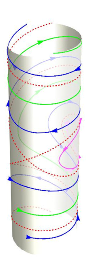
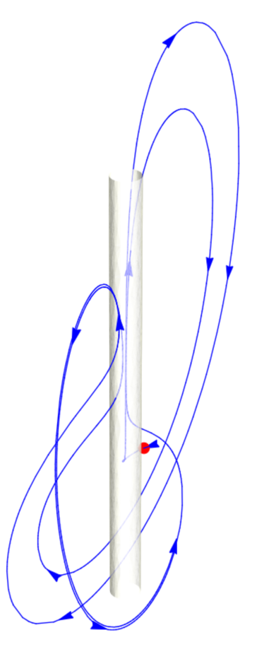
Figure 1: (Color online) — (a) Representative trajectories of the $\mathcal{PT}$-symmetric coupler on the surface of a cylinder. A periodic trajectory — the closed solid curve in the middle of the cylinder, plotted in purple (gray) — is confined within the separatrix loop (plotted in dashed red). The other two solid curves — dark blue (black) and green (light gray) — wind up to $Z\to\infty$ and represent blow-up regimes of the coupler. Here $\gamma=0.5$ and $\rho=3$. (b) A representative trajectory of the $\mathcal{AC}$-coupler. From the point shown by the red blob, the trajectory zaps onto the vertical axis, starts moving up, but gradually deviates from the vertical and leaves the imaginary cylinder of small radius. The trajectory ends up approaching a limit cycle. The blowup is arrested. Here $\gamma=1.9$, $a=2$ and the initial conditions $(X,Y,Z)=(0,5,0)$.

Using (12), Eqs.(8) and (9) become

$${\dot{\theta}}=Z,\quad{\dot{Z}}=\gamma^{2}(\theta-\chi)-\rho\cos\theta.$$ (14)

This has an obvious conservation law:

$${\dot{\theta}}^{2}-\gamma^{2}(\theta-\chi)^{2}+2\rho\sin\theta+\rho^{2}+1=0,$$ (15)

where we used (13) to identify the constant of integration. This is an equation for a curve on the surface of a cylinder of radius $\rho$. The curve is determined by the angular parameter $\chi$.

The cylindrical radius $\rho$ and the angle $\chi$ are two integrals of motion of the $\mathcal{PT}$-symmetric dimer (1). The availability of two independent integrals makes the dimer a completely integrable system RKEC .

The cylinder of the radius $\rho=0$ is exceptional. When $\rho=0$, $\theta$ is undefined and Eq.(15) is invalid. However, in this case Eq.(7c) gives ${\dot{Z}}=\gamma\sqrt{Z^{2}+1}$, whence $Z=\sinh[\gamma(t-t_{0})]$. This is the trajectory corresponding to our explicit blowup solution (5). (See also Pickton .)

We note that equations similar to (14) were derived in KPT ; Pickton within a different formalism.

II.3 Imaginary particle representation

Assume $\rho\neq 0$, and let $\kappa=\gamma/\sqrt{2\rho}>0$. Denoting $\tau=\sqrt{\rho}t$ and $q=\theta-\chi$, Eq.(15) acquires the form of the energy conservation law for a classical particle in the potential $V(q)$:

$$\frac{{q_{\tau}}^{2}}{2}+V(q)=E.$$ (16)

Here

$$E=-1-\frac{(\rho-1)^{2}}{2\rho}$$ (17)

and the potential

$$V(q)=-\kappa^{2}q^{2}+\sin(q+\chi).$$ (18)

Since

$$\rho^{2}+2\rho\sin(q+\chi)+1\geq(\rho-1)^{2}\geq 0,$$

it follows from Eq.(16) that $|q_{t}|\leq\gamma|q|$. Letting $q=q(0)e^{\phi}$ yields $|\phi_{t}|\leq\gamma$, and so

$$|q(0)|e^{-\gamma t}\leq|q|\leq|q(0)|e^{\gamma t}.$$ (19)

This inequality implies that $q$ cannot grow faster than $e^{\gamma t}$. (This result was previously established via the balance equations KPT .)

According to (13), adding a multiple of $2\pi$ to $\theta$ changes $\chi$ but does not affect $q$. Therefore without loss of generality $\chi$ can be taken in the interval $(0,2\pi)$.

It is not difficult to realise that not all trajectories of the imaginary particle correspond to evolutions of the system (1). First of all, the value of $E$ in (17) is bounded from above: $E\leq-1$. Therefore only trajectories of the particle with $E\leq-1$ correspond to the dimer’s trajectories on the surface of a cylinder with some $\rho$ (and $\gamma$ given by $\sqrt{2\rho}\kappa$).

Second, in view of (12), only positive $q$ represent configurations of the dimer. Any trajectory of the particle with $q$ reaching zero, or approaching zero as $\tau$ grows to infinity, would correspond to a solution of the system (1) decaying to zero, in finite or infinite time: $|\psi_{1}|^{2}+|\psi_{2}|^{2}\to 0$. [In the next subsection, we will show that the specific choice of the integration constant in (16) is compatible with only one such trajectory.]

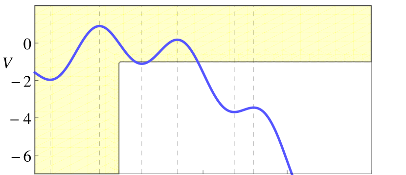
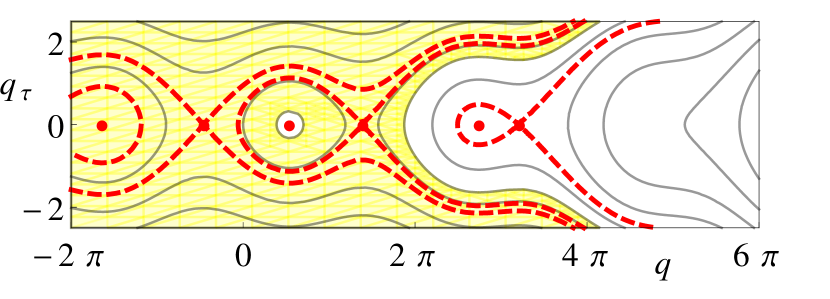
Figure 2: (Color online) — Top: the potential $V(q)=\sin(q+\chi)-\kappa^{2}q^{2}$, with the vertical lines indicating positions of the extrema. Here $\kappa=0.2$ and $\chi=\pi$. The negative $q$ and the potential values $V>-1$ are inaccessible to the imaginary particle (shaded in yellow). Bottom: the corresponding phase portrait with fixed points and separatrices shown in dashed red, calculated via Eq.(16). Shaded is the region where $q<0$ or $E>-1$. Trajectories in this region do not correspond to any motions of the dimer.

The top panel in Fig.2 sketches a potential $V(q)$ for a particular set of values of $\kappa$ and $\chi$. Shaded is the region where $q<0$ and the section with $V>-1$. The bottom panel shows trajectories of the imaginary particle moving in this potential, for several values of $E$. Again, shaded is the portion of the phase space where $q<0$ or $E>-1$. Evolutions of the dimer are represented by the trajectories in the region that was left blank.

When $\gamma=0$, we have $r=const$ instead of Eq.(12). In this case, Eq.(16) is replaced with the pendulum equation:

$$\frac{{\dot{\theta}}^{2}}{2\rho}+\sin\theta=E.$$ (20)

Here $E$ is determined by the initial conditions: $E=\sin\theta(0)+\frac{1}{2}Z^{2}(0)/\rho(0)$. The elliptic-function solution of (20) can be found in standard textbooks. The pendulum is librating when $-1\leq E\leq 1$ and rotating when $E\geq 1$. When averaged over a long interval, the $\theta$-coordinate of the rotating pendulum grows as a linear function of $t$.

II.4 Fixed points

The fixed points of the two-dimensional system (14) satisfy

$$2\kappa^{2}q=\cos(q+\chi).$$ (21)

This equation has $2N+1$ roots, $q^{(0)},q^{(1)},...,q^{(2N)}$, where $N$ depends on $\kappa$ and $\chi$. For $2\kappa^{2}>1$, there is only one point, of saddle type, irrespectively of the value of $0\leq\chi<2\pi$. As $\kappa\to\infty$, this fixed point is given by the asymptotic expression

$$q^{(0)}=\frac{\cos\chi}{2\kappa^{2}}-\frac{\sin 2\chi}{8\kappa^{4}}+O(\kappa^{-6}).$$ (22)

Assume now that the parameter $2\kappa^{2}$ is being decreased from $1$. For a generic value of $\chi$, a pair of new fixed points is born in a saddle-node bifurcation as $\kappa$ passes through $\kappa_{n}$ or ${\tilde{\kappa}_{n}}$, where $\kappa_{n}$ is defined as the root of the equation

$$f(\kappa_{n})=2\pi n-\chi,\quad n=1,2,...,$$ (23)

and ${\tilde{\kappa}_{n}}$ as the root of

$$f({\tilde{\kappa}_{n}})=\chi+\pi+2\pi n,\quad n=0,1,2,....$$ (24)

Here the function

$$f(\kappa)=\frac{1}{2\kappa^{2}}\sqrt{1-4\kappa^{4}}+\arcsin(2\kappa^{2})$$

is monotonically decreasing from $\infty$ to $\pi/2$ as $2\kappa^{2}$ grows from 0 to 1. The equations (23) and (24) are arrived at by eliminating $q$ between (21) and the bifurcation condition

$$2\kappa^{2}+\sin(q+\chi)=0.$$ (25)

The values $\chi=\pi/2$ and $\chi=3\pi/2$ are exceptional as these are associated with enhanced symmetry of Eq.(21). In each of these two cases both sides of Eq.(21) are given by odd functions of $q$; hence two pairs of fixed points are born on crossing $\kappa_{n}$ or ${\tilde{\kappa}_{n}}$. (When $\chi=\pi/2$, we have $\kappa_{n+1}={\tilde{\kappa}_{n}}$; when $\chi=3\pi/2$, the correspondence is $\kappa_{n+2}={\tilde{\kappa}_{n}}$.)

The order of the bifurcation points depends on $\chi$. We have

$$0<...\leq\kappa_{3}\leq{\tilde{\kappa}_{2}}\leq\kappa_{2}\leq{\tilde{\kappa}_{1}}\leq\kappa_{1}\leq{\tilde{\kappa}_{0}}\leq\frac{1}{\sqrt{2}}$$

when $0\leq\chi\leq\pi/2$;

$$0<...\leq{\tilde{\kappa}_{2}}\leq\kappa_{3}\leq{\tilde{\kappa}_{1}}\leq\kappa_{2}\leq{\tilde{\kappa}_{0}}\leq\kappa_{1}\leq\frac{1}{\sqrt{2}}$$

when $\pi/2\leq\chi\leq 3\pi/2$, and, finally,

$$0<...\leq\kappa_{4}\leq{\tilde{\kappa}_{1}}\leq\kappa_{3}\leq{\tilde{\kappa}_{0}}\leq\kappa_{2}\leq\kappa_{1}\leq\frac{1}{\sqrt{2}}$$

when $\chi\geq 3\pi/2$.

It is important to emphasise that the phase portrait given in Fig.2 cannot be simply “wrapped” around the cylindrical surface in Fig.1. Different trajectories shown in Fig.2 pertain to cylinders with different $\rho$; in particular, different fixed points belong to different cylinders. A natural question is how many fixed points lie on the surface of the cylinder of a given radius.

To answer this, we calculate the value of the potential $V(q)$ at its points of extrema:

$$V(q^{(m)})=W(\sin(q^{(m)}+\chi)),$$

where

$$W(y)=-1+\frac{(y+1)(y+4\kappa^{2}-1)}{4\kappa^{2}}.$$ (26)

When $2\kappa^{2}\geq 1$ (that is, when $\rho\leq\gamma^{2}$), the function $W(y)$ lies above -1 when $y$ is in the interval $-1\leq y\leq 1$. On the other hand, the maximum of the energy (17), attained at $\rho=1$, equals -1. Therefore, cylinders with $\rho\leq\gamma^{2}$ do not have fixed points — except when $\rho=1$. (This exceptional situation is obviously arising only if $\gamma>1$.)

The cylinder with $\rho=1$ is special as it contains the origin $X=Y=Z=0$. When $\gamma>1$, the two-dimensional system (14) with $\rho=1$ and $\chi=3\pi/2$ has a saddle point at $q=0$. Unlike the saddles and centers in systems with other $\rho$ and $\chi$, this fixed point is accessible to the particle. In this case, Eq.(16) has the form

$$\frac{q_{\tau}^{2}}{2}-\frac{\gamma^{2}}{2}q^{2}+2\sin^{2}\frac{q}{2}=0.$$ (27)

The stable manifold of the saddle describes the solution of the dimer (1) with $|\psi_{1}|^{2}+|\psi_{2}|^{2}\to 0$ as $z\to\infty$. On the other hand, the initial conditions $(q,q_{\tau})$ constituting the unstable manifold give rise to the blow-up regimes, $|\psi_{1}|^{2}+|\psi_{2}|^{2}\to\infty$ as $z\to\infty$.

When $2\kappa^{2}\leq 1$ (i.e. $\rho\geq\gamma^{2}$), the function $W(y)$ has a (single) minimum, at $y=-2\kappa^{2}$, with

$$W_{\rm min}=W(-2\kappa^{2})=-1-\frac{\gamma^{2}}{2\rho}\left(1-\frac{\rho}{\gamma^{2}}\right)^{2}.$$ (28)

Therefore, cylinders with $W_{\rm min}<E$ will have two fixed points each. Substituting from (17) for $E$, this inequality reduces to

$$(1-\gamma^{2})(\rho-\gamma)>0.$$ (29)

When $\gamma<1$, the inequality (29) requires $\rho>\gamma$. Here, the fixed points are at $\theta_{1,2}=\arcsin y_{1,2}$, where

$$y_{1,2}=-\frac{\gamma^{2}}{\rho}\pm\frac{\sqrt{(1-\gamma^{2})(\rho^{2}-\gamma^{2})}}{\rho}.$$

The type of the fixed point — considered as a fixed point of the imaginary particle — is determined by the second derivative of $V(q)$:

$$\frac{\partial^{2}V}{\partial q^{2}}=-\frac{\gamma^{2}}{\rho}-\sin(q+\chi).$$

Substituting $y_{1,2}$ for $\sin(q+\chi)$, we verify that $\theta_{1}$ is a saddle ($\frac{\partial^{2}V}{\partial q^{2}}<0$) while $\theta_{2}$ is a centre ($\frac{\partial^{2}V}{\partial q^{2}}>0$).

On the other hand, when $\gamma>1$ the inequality (29) requires $\rho<\gamma$. However this is incompatible with our assumption $\rho>\gamma^{2}$, because $\gamma^{2}$ becomes greater than $\gamma$ if $\gamma>1$.

Since the system (14) is conservative, each centre point is encircled by closed curves on the $(q,q_{\tau})$ plane. Furthermore, it is not difficult to realise that each centre point is surrounded by closed oribts on the cylindrical surface it belongs to (see Fig.1). Indeed, let $V_{\chi}$ be the potential (18) corresponding to the parameter value $\chi$, denote $q^{(m)}(\chi)$ the corresponding roots of Eq.(21) and let $\rho(\chi)$ be the cylinder radius defined as a root of $V_{\chi}(q^{(m)}(\chi))=E$, with $E$ as in (17). Since

$$\left.\frac{\partial V_{\chi}(q)}{\partial\chi}\right|_{q^{(m)}}=\cos(q^{(m)}+\chi)=2\kappa^{2}q^{(m)}>0,$$

the value $V_{\chi^{\prime}}(q^{(m)}(\chi))$, where $\chi^{\prime}=\chi+\delta\chi$ and $\delta\chi<0$ is a small perturbation, will be lower than $V_{\chi}(q^{(m)}(\chi))$ by a small amount. Therefore the conservation law (16) with $V_{\chi^{\prime}}$ will describe a periodic trajectory of small radius on the surface of the cylinder $\rho(\chi)$. The trajectory will enclose the fixed point $q^{(m)}(\chi^{\prime})$.

In summary, we need to distinguish between the situations with $\gamma<1$ and $\gamma>1$. When $\gamma<1$, cylinders of small radius $\rho<\gamma$ do not harbour any fixed points; all trajectories are unbounded. On the other hand, cylinders of radius $\rho>\gamma$ feature two fixed points, a centre and a saddle; in this case periodic orbits arise in addition to the unbounded motions. Finally, there are no fixed points if $\gamma>1$. (The only exception is the cylinder with $\rho=1$ which has the saddle point at the origin, $r=0$.) All trajectories are spiralling up to infinity (except the stable manifold of the saddle at $\rho=1$).

After this paper has been submitted for publication, we have learnt of the preprint Pickton where the unboundedness of trajectories for $\gamma>1$ was obtained within a different formalism.

II.5 Symmetry-broken phase

The blowup of generic initial conditions in the symmetry-broken phase ($\gamma>1$) may be demonstrated without appealing to details of the phase portrait. We now demonstrate this fact simply by considering the power imbalance between the two waveguides.

First, we show that in this symmetry-broken phase, all initial conditions with $P_{1}>P_{2}$ blow up. From Eq.(1) it follows that

$$\frac{d}{dz}(P_{1}-P_{2})=2(\gamma-1)(P_{1}+P_{2})$$

$$+2(P_{1}+P_{2})+2i(\psi_{1}^{*}\psi_{2}-\psi_{1}\psi_{2}^{*})$$

$$\geq 2(\gamma-1)(P_{1}+P_{2})+2(\sqrt{P_{1}}-\sqrt{P_{2}})^{2},$$ (30)

whence

$$\frac{d}{dz}(P_{1}-P_{2})\geq 2(\gamma-1)(P_{1}-P_{2}).$$

By the Gronwall inequality, the difference $P_{1}-P_{2}$ tends to infinity for any initial conditions with $P_{1}(0)>P_{2}(0)$. That is, any initial conditions with $P_{1}(0)>P_{2}(0)$ lead to a blow-up.

Most of solutions with $P_{2}(0)\geq P_{1}(0)$ will also blow up. To show this, we first observe that Eq.(30) implies

$$\frac{d}{dz}(P_{2}-P_{1})$$

$$\leq-2(\gamma-1)(P_{1}+P_{2})-2(\sqrt{P_{2}}-\sqrt{P_{1}})^{2}<0.$$ (31)

According to (31), the quantity $P_{2}-P_{1}$ must decrease until $P_{2}=P_{1}$. If $P_{1}$ and $P_{1}$ are not zero at the moment when they become equal, the difference $P_{2}-P_{1}$ will continue to decrease. Once the difference $P_{2}-P_{1}$ has become negative, the system is in the blowup regime described above.

The quantities $P_{1}$ and $P_{2}$ may simultaneously go to zero only if $\rho=1$. Indeed, the product $P_{1}P_{2}$ equals $X^{2}+Y^{2}$ while

$$X^{2}+Y^{2}=(\rho-1)^{2}+2\rho(1+\sin\theta)\geq(\rho-1)^{2};$$

hence $P_{1}P_{2}\geq(1-\rho)^{2}$. The trajectory with $P_{1}$, $P_{2}\to 0$ is the stable manifold of the saddle point $\rho=1$, $\theta=3\pi/2$, $Z=0$ (that is, of the point $X=Y=Z=0$).

In conclusion, in the symmetry-broken phase ($\gamma>1$), all initial conditions lead to the blowup of solutions, except initial conditions that lie on the stable manifold of the saddle point $\psi_{1}=\psi_{2}=0$.

III $\mathcal{AC}$ dimer

The $\mathcal{AC}$ coupler offers an alternative to the $\mathcal{PT}$-symmetric configuration of gain and loss ABRF . The arrangement consists of two lossy waveguides placed in an active medium. Instead of providing power gain in the core of (one of the) waveguides, the structure boosts the evanescent fields which couple the two channels due to their close proximity.

The optical field in the two guides is described by the amplitudes $\psi_{1}$ and $\psi_{2}$. These satisfy

$$i\frac{d\psi_{1}}{dz}+\beta|\psi_{1}|^{2}\psi_{1}+\psi_{2}=-i\gamma\psi_{1}+ia\psi_{2},$$ (32a)

$$i\frac{d\psi_{2}}{dz}+\beta|\psi_{2}|^{2}\psi_{2}+\psi_{1}=-i\gamma\psi_{2}+ia\psi_{1}.$$ (32b)

Here $a$ and $\gamma>0$ are the gain and loss coefficient, respectively. We assume $a>\gamma$ (because if $a<\gamma$, all solutions decay to zero ABRF ). The coefficient $\beta$ measures the strength of nonlinearity. The choice $\beta>0$ corresponds to the focusing and $\beta<0$ to defocusing nonlinearity.

We note that a closely related system, with $\beta<0$, describes radiative coupling and weak lasing of exciton-polariton condensates Aleiner . Unlike the $\mathcal{PT}$-symmetric dimer, the $\mathcal{AC}$ couplers with the opposite sign of $\beta$ are not equivalent. The staggering transformation (3) changes the sign of $a$ in addition to the sign of the nonlinear term. If the sign of $a$ is fixed by the condition $a>\gamma>0$, the cases $\beta>0$ and $\beta<0$ have to be considered independently.

Linearising (32) about $\psi_{1,2}=0$ one checks that the symmetric part of the small perturbation, $u=\psi_{1}+\psi_{2}$, gains energy and grows:

$$u(z)=u(0)e^{(i+a-\gamma)z}.$$

On the other hand, the antisymmetric normal mode, $v=\psi_{1}-\psi_{2}$, loses energy and decays to zero:

$$v(z)=v(0)e^{-(i+a+\gamma)z}.$$

The numerical evidence ABRF is that the nonlinearity which couples the two modes, may drain the energy gained by the symmetric mode through the antisymmetric channel. Below, we study the blowup arrest analytically, and identify the type of nonlinearity capable of this job.

The system (32) has two invariant manifolds. One is defined by the reduction $\psi_{1}=\psi_{2}\equiv\psi$, where $\psi$ satisfies

$$i\frac{d\psi}{dz}+\beta|\psi|^{2}\psi+\psi=i(a-\gamma)\psi,$$ (33)

and the other one by $\psi_{1}=-\psi_{2}=\psi$, where

$$i\frac{d\psi}{dz}+\beta|\psi|^{2}\psi-\psi=-i(a+\gamma)\psi.$$ (34)

All solutions of (34) decay to zero; letting $|\psi(0)|^{2}=A^{2}$, we have

$$\psi(z)=\psi(0)e^{-(a+\gamma)z+i(\beta A^{2}-1)z}.$$ (35)

On the other hand, all solutions of (33) blow up, exponentially:

$$\psi(z)=\psi(0)e^{(a-\gamma)z+i(\beta A^{2}+1)z}.$$ (36)

The issue we are exploring in what follows, is whether initial conditions that lie close to the “blow-up manifold” $\psi_{1}=\psi_{2}$ blow up as well.

Performing the polar decomposition of the fields $\psi_{1}=\sqrt{P_{1}}e^{i\Phi_{1}}$ and $\psi_{2}=\sqrt{P_{2}}e^{i(\Phi_{2})}$, one checks that $\Phi_{1}$ can be separated from the other three variables. This phase variable satisfies

$${\dot{\Phi}_{1}}=\frac{\beta(r+X)}{2}+\frac{Z+aX}{2(r+X)},$$

while the remaining equations of motion can be written as

$${\dot{X}}=-\gamma X-Y,$$ (37a)

$${\dot{Y}}=-\gamma Y+X-\beta XZ,$$ (37b)

$${\dot{Z}}=-\gamma Z+ar+\beta XY.$$ (37c)

Here $X=\frac{1}{2}(|\psi_{1}|^{2}-|\psi_{2}|^{2})$ measures the power imbalance between the two waveguides; $Y=\frac{i}{2}(\psi_{1}\psi_{2}^{*}-\psi_{1}^{*}\psi_{2})$ characterizes the energy flux from the first to the second channel, and $2aZ$ — where $Z=\frac{1}{2}(\psi_{1}\psi_{2}^{*}+\psi_{2}\psi_{1}^{*})$ — is the total gain in the system. The Stokes variables $X,Y$, and $Z$ are three components of the vector ${\bf r}$, with $r=\sqrt{{\bf r}^{2}}=\frac{1}{2}(P_{1}+P_{2})$. [Note that the Stokes variables have been introduced differently from (6); this is done in order to elucidate parallels in the geometry of the phase spaces of the two systems.] The overdot indicates differentiation with respect to the fictitious time variable, $t=2z$, which we introduce for convenience of analysis.

III.1 Defocusing nonlinearity

With the $\mathcal{AC}$ dimer being only recently introduced, its phenomenology still needs to be elucidated. One issue that requires a careful investigation is the type of nonlinearity that is necessary for the operation of the structure as an optical coupler. The choice of the self-focussing Kerr nonlinearity in the original version of this structure ABRF was arbitrary; the defocussing nonlinearity could have been an equally acceptable candidate.

In this subsection we show, however, that the defocussing cubic nonlinearity ($\beta<0$) is unable to prevent the blow-up.

Our analysis makes use of the function

$${\mathcal{L}}=Z+\frac{\beta}{2}X^{2},$$ (38)

which satisfies

$${\dot{\mathcal{L}}}=ar-\gamma Z-\gamma\beta X^{2}.$$ (39)

We start by considering the initial conditions $X,Y,Z$ such that ${\mathcal{L}}\leq 0$. From the definition of $\mathcal{L}$ we have $-\beta X^{2}\geq 2Z$. Using this inequality in (39) we obtain

$${\dot{\mathcal{L}}}\geq ar+\gamma Z\geq(a-\gamma)|Z|.$$

This means that ${\mathcal{L}}(t)$ will either grow until it is positive, or tend to zero as $t\to\infty$. The latter is only possible if the initial condition lies on the stable manifold of the origin [described by Eq.(35)].

Thus we need to consider only initial conditions satisfying ${\mathcal{L}}(0)>0$. When $\beta<0$, Eq.(39) implies

$${\dot{\mathcal{L}}}\geq(a-\gamma)r.$$ (40)

Since $\mathcal{L}\leq r$ and so ${\dot{\mathcal{L}}}\geq(a-\gamma){\mathcal{L}}$, the Gronwall inequality gives ${\mathcal{L}}(t)\geq{\mathcal{L}}(0)e^{(a-\gamma)t}$ for any initial conditions with ${\mathcal{L}}(0)>0$. This means that these initial conditions blow up: $|\psi_{1}|^{2}+|\psi_{2}|^{2}\to\infty$ as $z\to\infty$. (From the structure of $\mathcal{L}$ it follows that $|\psi_{1}|$ and $|\psi_{2}|$ grow to infinity at the same rate.)

Thus the defocusing nonlinearity cannot arrest the blowup of solutions of the linear ${\mathcal{A}C}$-dimer. In what follows we concentrate on the focusing case ($\beta>0$) and scale $\psi_{1,2}$ so that $\beta=1$.

III.2 Instability of the blowup solution

Here our purpose is to explore trajectories that start in the vicinity of the blow-up manifold (36). In terms of $X,Y$ and $Z$, this manifold is given by the positive vertical axis: $X=Y=0$; $Z>0$. We wish to determine whether these trajectories escape to infinity or remain in the finite part of the space.

In terms of the cylindrical coordinates Eqs.(37) acquire the form

$${\dot{\rho}}=\left[-\gamma-\frac{1}{2}Z\sin(2\theta)\right]\rho,$$ (41a)

$${\dot{Z}}=-\gamma Z+a\sqrt{\rho^{2}+Z^{2}}+\frac{1}{2}\rho^{2}\sin(2\theta),$$ (41b)

$${\dot{\theta}}=1-Z\cos^{2}\theta.$$ (41c)

Here $X=\rho\cos\theta$ and $Y=\rho\sin\theta$.

We assume that the motion starts in a narrow cylinder around the $Z$ axis, and linearise in small $\rho$. Equation (41b) is then simply ${\dot{Z}}=(a-\gamma)Z$, so that $Z$ grows: $Z(t)=Z(0)e^{2\lambda t}$, where $2\lambda=a-\gamma$. Assume that $Z(0)>1$ while $\theta(0)$ is in the vicinity of $\pi/2$ or $-\pi/2$. Writing $\theta=\pm\pi/2+\epsilon(t)$, Eq.(41c) becomes

$${\dot{\epsilon}}=1-Z(t)\epsilon^{2},\quad Z=Z(0)e^{2\lambda t}.$$

The solution of this Riccati equation is

$$\epsilon=\frac{\lambda}{Z}+\lambda\frac{d}{dZ}\ln\left[K_{1}\left(\frac{\sqrt{Z}}{\lambda}\right)+CI_{1}\left(\frac{\sqrt{Z}}{\lambda}\right)\right]^{2},$$ (42)

where $I_{1}(w)$ and $K_{1}(w)$ are the modified Bessel functions of order one, and $C$ is a constant of integration. As $Z$ grows, (42) gives $\epsilon\to\pm 1/\sqrt{Z}$, where the top respectively bottom sign results from choosing $C\neq 0$ respectively $C=0$.

When $\theta$ approaches $\pi/2$ from below ($\epsilon<0$) or $-\pi/2$ from above ($\epsilon>0$), the contents of the square bracket in (41a) tends to $-\gamma-\sqrt{Z}$. The radius $\rho(t)$ continues to decrease while $Z$ continues to grow. The trajectory is captured in a blowup regime.

On the other hand, when $\theta$ tends to $\pi/2$ from above or $-\pi/2$ from below, the square bracket becomes $\sqrt{Z}-\gamma$, which is large and positive. The radius $\rho$ then starts increasing as a double exponential function, and the last, negative, term in (41b) outgrows the first two terms. This suppresses any further growth of $Z$; the trajectory moves away from the blowup manifold [Fig.1(b)].

When $\rho(0)$ is small, a tiny perturbation is sufficient to change the sign of $\epsilon(0)$ and divert the phase point from a trajectory escaping to infinity. Therefore, even though there are trajectories with $X,Y\to 0$, $Z\to\infty$ as $t\to\infty$, these blowup solutions are unstable and will not be observed in any practical situation. (In particular, the blowup cannot be observed in numerical simulations of the $\mathcal{AC}$ dimer.)

IV Conclusions

In the case of the $\mathcal{PT}$ symmetric dimer, our results include the following.

(1) In the symmetry-broken phase ($\gamma>1$) we have demonstrated that all initial conditions (except initial conditions from a special degenerate class) blow up.

(2) We have elucidated the geometry of the phase space of the dimer. In particular, we have shown that the phase space is foliated into coaxial two-dimensional cylinders. Cylinders of small radius only harbor trajectories that escape to infinity; these describe the blow-up regimes of the dimer. When $\gamma\leq 1$, cylinders with larger radii host periodic trajectories in addition to the unbounded motions.

An implication of the phase space foliation and the conservativity of motion on each cylinder, is that the blow-up regime is stable. Small perturbations may shift the phase point around the cylindric surface, or push it from one cylinder to another, but this will not take it to the bounded trajectories. The evolution carries the phase point further away from the domains of finite motion.

For the $\mathcal{AC}$ dimer, we have established that

(1) The defocusing Kerr nonlinearity is unable to suppress the blowup. Generic initial conditions lead to unbounded trajectories.

(2) The phase space of the $\mathcal{AC}$ dimer is genuinely three-dimensional and not foliated. When the nonlinearity is focussing, there is a domain of initial conditions occupying nonzero phase volume, that lead to blow-up regimes. However all the unbounded trajectories lie within a rapidly narrowing funnel centered on the vertical axis. The blow-up funnel is unstable: a small perturbation is sufficient to kick a trajectory out of the funnel and send it towards a stable limit cycle.

In conclusion, the same, focussing cubic, nonlinearity plays a dramatically different role in the dynamics of the $\mathcal{PT}$ and $\mathcal{AC}$ dimer. In the $\mathcal{PT}$-symmetric arrangement of the gain and loss, the nonlinearity promotes the blowup of solutions. In the case of the $\mathcal{AC}$ coupler, the nonlinearity suppresses the blowup by coupling the linearly excitable to the linearly damped normal mode. We have shown that this opposite effect of the nonlinearity is due to the difference in the geometry of the phase space of the two systems.

References

References

- (1) S. Klaiman, U. Günther, and N. Moiseyev, Phys. Rev. Lett. 101 080402 (2008); Z. Lin, H. Ramezani, T. Eichelkraut, T. Kottos, H. Cao, and D. N. Christodoulides, Phys. Rev. Lett. 106 213901 (2011); A. Regensburger, C. Bersch, M.-A. Miri, G. Onishchukov, D. N. Christodoulides, and U. Peschel, Nature 488 167 (2012)
- (2) A.A. Sukhorukov, Z.Y. Xu, Yu.S. Kivshar, Phys. Rev. A 82 043818 (2010)
- (3) C. E. Rüter, K. G. Makris, R. El-Ganainy, D.N. Christodoulides, M. Segev, and D. Kip, Nat. Phys. 6 192 (2010); T. Kottos, ibid. 166.
- (4) K. G. Makris, R. El-Ganainy, D. N. Christodoulides, and Z. H. Musslimani, Phys. Rev. Lett. 100 103904 (2008)
- (5) M. C. Zheng, D. N. Christodoulides, R. Fleischmann, T. Kottos, Phys. Rev. A 82 010103 (2010)
- (6) S. Longhi, Phys. Rev. Lett. 103 123601 (2009)
- (7) A. Guo, G. J. Salamo, D. Duchesne, R. Morandotti, M. Volatier-Ravat, V. Aimez, G. A. Siviloglou, and D. N. Christodoulides. Phys. Rev. Lett. 103 093902 (2009)
- (8) H. Ramezani, T. Kottos, V. Kovanis, and D. N. Christodoulides, Phys. Rev. A 85 013818 (2012)
- (9) I. V.Barashenkov, S. V. Suchkov, A. A. Sukhorukov, S. V. Dmitriev, and Y. S. Kivshar, Phys. Rev. A 86 053809 (2012)
- (10) H. Ramezani, T. Kottos, R. El-Ganainy, and D.H. Christodoulides, Phys. Rev. A 82 043803 (2010)
- (11) S. Hu and W. Hu, J. Phys. B: At. Mol. Opt. Phys. 45 225401 (2012); Y. He and D. Mihalache, Phys. Rev. A 87 013812 (2013); Y. V. Bludov, V. V. Konotop, B. A. Malomed, Phys. Rev. A 87 013816 (2013); G. Della Valle, S. Longhi, Phys. Rev. A 87 022119 (2013); K. Li, D. A. Zezyulin, V. V. Konotop, P. G. Kevrekidis, Phys. Rev. A 87 033812 (2013); X. L. Shi, F. W. Ye, B. Malomed, X. F. Chen, Opt. Lett. 38 1064 (2013); M. Duanmu, K. Li, R. L. Horne, P. G. Kevrekidis, N. Whitaker, Phil. Trans. Roy. Soc. A - Math. Phys. Eng. Sci. 371 20120171 (2013); Y. V. Bludov, R. Driben, V. V. Konotop, B. A. Malomed, Journ. Optics 15 064010 (2013); S. Nixon, J. K. Yang, Optics Lett. 38 1933 (2013); B. Peng, Ṣ. K. Özdemir, F. Lei, F. Monifi, M. Gianfreda, G. L. Long, S. Fan, F. Nori, C. M. Bender, L. Yang, submitted to Nature (2013)
- (12) N. V. Alexeeva, I. V. Barashenkov, K. Rayanov, and S. Flach, arXiv: 1308.5862
- (13) Y. Chen, A. W. Snyder, and D. N. Payne, IEEE Journ. Quant. Electronics 28 239 (1992)
- (14) K. Li and P. G. Kevrekidis, Phys. Rev. E 83 066608 (2011); J. D’Ambroise, P. G. Kevrekidis, and S. Lepri, J. Phys. A Math. Theor. 45 (2012) 444012; D. A. Zezyulin and V. V. Konotop, Phys. Rev. Lett. 108 213906 (2012); K. Li, P. G. Kevrekidis, B. A. Malomed, and U. Günther, J. Phys. A: Math. Theor. 45, 444021 (2012); I. V. Barashenkov, L. Baker, N. V. Alexeeva, Phys. Rev. A 87 033819 (2013); P. G. Kevrekidis, D. E. Pelinovsky, and D. Y. Tyugin, J. Appl. Dynam. Syst. 12 1210 (2013)
- (15) S. V. Dmitriev, A. A. Sukhorukov, and Y. S. Kivshar, Opt. Lett. 35 2976 (2010); S. V. Suchkov, B. A. Malomed, S. V. Dmitriev, and Y. S.Kivshar, Phys. Rev. E 84 046609 (2011); R. Driben and B. A. Malomed, Opt. Lett. 36 4323 (2011); S. V. Suchkov, A. A. Sukhorukov, S. V. Dmitriev, Y. S. Kivshar, EPL 100 54003 (2012); D. E. Pelinovsky, P. G. Kevrekidis, D. J. Frantzeskakis, EPL 101 11002 (2013)
- (16) P. G. Kevrekidis, D. E. Pelinovsky, and D. Y. Tyugin, J. Phys. A: Math. Theor. 46 365201 (2013)
- (17) I. L. Aleiner, B. L. Altshuler, and Y. G. Rubo. Phys. Rev. B 85 121301 (2012)
- (18) J. Pickton and H. Susanto, arXiv: 1307.2788