Dark Energy from holographic theories with hyperscaling violation

Abstract

We show that analytical continuation maps scalar solitonic solutions of Einstein-scalar gravity, interpolating between an hyperscaling violating and an Anti de Sitter (AdS) region, in flat FLRW cosmological solutions sourced by a scalar field. We generate in this way exact FLRW solutions that can be used to model cosmological evolution driven by dark energy (a quintessence field) and usual matter. In absence of matter, the flow from the hyperscaling violating regime to the conformal AdS fixed point in holographic models corresponds to cosmological evolution from power-law expansion at early cosmic times to a de Sitter (dS) stable fixed point at late times. In presence of matter, we have a scaling regime at early times, followed by an intermediate regime in which dark energy tracks matter. At late times the solution exits the scaling regime with a sharp transition to a dS spacetime. The phase transition between hyperscaling violation and conformal fixed point observed in holographic gravity has a cosmological counterpart in the transition between a scaling era and a dS era dominated by the energy of the vacuum.

I Introduction

Triggered by the anti-de Sitter/Conformal field theory (AdS/CFT) correspondence, recently we have seen several application of the holographic principle aimed to describe the strongly coupled regime of quantum field theory (QFT) Hartnoll et al. (2008a, b); Horowitz and Roberts (2008); Charmousis et al. (2009); Cadoni et al. (2010); Goldstein et al. (2010); Gouteraux and Kiritsis (2012). The most interesting example of these applications is represented by the holographic description of quantum phase transitions, such as those leading to critical superconductivity and hyperscaling violation Hartnoll et al. (2008a, b); Charmousis et al. (2009); Gubser and Rocha (2010); Cadoni et al. (2010); Goldstein et al. (2010); Dong et al. (2012); Cadoni and Pani (2011); Huijse et al. (2012); Cadoni and Mignemi (2012); Cadoni and Serra (2012); Narayan (2012); Cadoni et al. (2013).

A general question that can be asked in this context is if these recent advances can be used to improve our understanding, not only of some holographic, strongly coupled dual QFT, but also of the gravitational interaction itself. After all the holographic principle in general and the AdS/CFT correspondence in particular, have been often used in this reversed direction. The most important example is without doubt the understanding of the statistical entropy of black holes by counting states in a dual CFT Strominger and Vafa (1996); Strominger (1998); Cadoni and Mignemi (1999).

A challenge for any theory of gravity is surely cosmology and in particular the understanding of the present accelerated expansion of the universe and the related dark energy hypothesis Peebles and Ratra (2003); Padmanabhan (2003). It is not a priori self-evident that the recent developments on the holographic side may be useful for cosmology McFadden and Skenderis (2010). However, closer scrutiny reveals that key concepts used in the holographic description can be also used in cosmology.

First of all the symmetries of the gravitational background. The AdS and de Sitter (dS) spacetime in $d$-dimensions share the same isometry group (the conformal group in $d-1$ dimensions). This fact has been the main motivation for the formulation of the dS/CFT correspondence Strominger (2001). Although this correspondence is problematic Goheer et al. (2003), it may be very useful to relate different gravitational backgrounds if one sees dS/CFT as analytical continuation $r\leftrightarrow it$ of AdS/CFT Cadoni and Carta (2004).

Second, a domain wall/cosmology correspondence has been proposed Skenderis and Townsend (2006); Skenderis et al. (2007); Shaghoulian (2013). For every supersymmetric domain-wall, which is solution of some supergravity (SUGRA) model, there is a corresponding flat Friedmann-Lemaitre-Robertson-Walker (FLRW) cosmology (which can be obtained by analytical continuation), of the same model but with opposite sign potential. This means that, although cosmologies in general cannot be supersymmetric they may allow for the existence of pseudo-Killing spinors.

Third, the spacelike radial coordinate $r$ of a static asymptotically AdS geometry can be interpreted as an energy scale and the corresponding dynamics as a renormalization group (RG) flow. This flow drives the dual QFT from an ultraviolet (UV) conformal fixed point (corresponding to the AdS geometry) to some nontrivial near-horizon, infrared (IR) point where only some scaling symmetries are preserved (for instance one can have hyperscaling violation in the IR Cadoni et al. (2013)). By means of the analytic continuation the RG flow becomes the cosmological dynamics of a time-dependent gravitational background, driving the universe from a early time regime (corresponding to the IR) to a late time regime (corresponding to the UV) Kiritsis (2013).

Last but not least, scalar fields play a crucial role both for holographic models and for cosmology. In the first case they are seen as scalar condensates triggering symmetry breaking and/or phase transitions in the dual QFT Hartnoll et al. (2008a, b); Cadoni et al. (2010). They are dual to relevant operators that drive the RG flow from the UV fixed point to the IR critical point. Moreover, they are the sources of scalar solitons, which are the gravitational background bridging the asymptotic AdS region and the near-horizon region. On the cosmological side it is well-known that scalar fields can be used to model dark energy (the so-called quintessence fields) Ford (1987); Wetterich (1988); Caldwell et al. (1998); Zlatev et al. (1999); Amendola and Tsujikawa (2010).

In this paper we will consider a wide class of Einstein-scalar gravity model (parametrized by a potential $V$) that have scalar solitonic solution interpolating between an hyperscaling violating region and an AdS region. These models have been investigated for holographic applications Charmousis et al. (2009); Cadoni et al. (2010); Goldstein et al. (2010); Dong et al. (2012); Cadoni and Pani (2011); Cadoni and Mignemi (2012); Cadoni and Serra (2012); Narayan (2012); Cadoni et al. (2013). We show that an analytical continuation transforms the solitonic solution in a flat FLRW solution of a model with opposite sign of $V$. If the soliton has the AdS region in the UV (IR), the FLRW solution will have a dS epoch at late (early) times. Correspondingly, the FLRW solution will be characterized by power-law expansion at early (late) times ( Section II).

Focusing on a particular Einstein-scalar model (parametrized by a parameter $\beta$) that has the AdS regime in the UV and for which exact solitonic solutions are known Cadoni et al. (2011), we generate (and characterize in detail) the corresponding flat FLRW exact solutions. For a broad range of $\beta$ the solutions describe a flat universe decelerating at early times but accelerating at late times (Section III).

We proceed by showing that these solutions can be used as a model for dark energy, the scalar field playing the role of a quintessence field. The parameter of state describing dark energy decreases with cosmic time, from a positive value ($<1$) till $-1$ (Section IV).

Finally, we discuss the cosmological dynamics in presence of matter in the form of a general perfect fluid. Although we are not able to solve exactly the coupled system, we give strong evidence that the universe naturally evolves from a scaling era at early times to a, cosmological constant dominated, de Sitter universe at late times. Moreover, the transition between the two regimes in not smooth and is the cosmological analogue of the hyperscaling violation/AdS spacetime phase transition of holographic models Cadoni et al. (2010, 2013); Gouteraux and Kiritsis (2012) (Section V).

II Dark energy, holographic theories and hyperscaling violation

We consider Einstein gravity coupled to a real scalar field $\phi$ in four dimensions:

$$I=\int d^{4}x\sqrt{-g}\left[{\cal{R}}-\frac{1}{2}\left(\partial\phi\right)^{2}-V(\phi)\right],$$ (1)

where ${\cal{R}}$ is the scalar curvature of the spacetime. The model is parametrized by the self-interaction potential $V(\phi)$ for the scalar field.

For static, radially symmetric solutions with planar topology for the transverse space, one can use the following parametrization of the solution:

$$ds^{2}=-U(r)dt^{2}+\frac{dr^{2}}{U(r)}+R^{2}(r)(dx^{2}+dy^{2}),\quad\phi=\phi(r).$$ (2)

It is known that the theory (1) admits solutions (2) describing black branes with scalar hair, at least for specific choices of $V(\phi)$ Cadoni et al. (2011, 2012); Cadoni and Mignemi (2012); Cadoni et al. (2013). When the spacetime is asymptotically AdS

$$U=R^{2}=\left(\frac{r}{R_{0}}\right)^{2}$$ (3)

(where $R_{0}$ is the AdS length) or more generically scale-covariant

$$U=R^{2}=\left(\frac{r}{r_{-}}\right)^{\eta},$$ (4)

(where $r_{-}$ and $0\leq\eta\leq 2$ are parameters), usual no-hair theorems can be circumvented and regular, hairy black brane solutions of (1) are allowed Cadoni et al. (2011, 2012).

Moreover, it has been shown that the zero-temperature extremal limit of these black brane solutions is necessarily characterized by $U=R^{2}$ in Eq. (2) Cadoni et al. (2011, 2013). The extremal limit describes a regular scalar soliton interpolating between an AdS spacetime and a scale-covariant metric. In particular, the behaviour of the potential at $r=\infty$ and in the near-horizon region determines the corresponding geometry. When the leading term of the potential is a constant $V(\phi)\sim-6/R_{0}^{2}$ the geometry is AdS. On the other hand if the potential behaves exponentially $V(\phi)\sim-e^{\lambda\phi}$ ($\lambda$ is some constant) we get a scale-covariant metric Cadoni et al. (2011).

The AdS vacuum has isometries generated by the conformal group in three dimensions. In particular the AdS metric is invariant under scale transformations:

$$r\to\mu^{-1}r,\quad(t,x,y)\to\mu(t,x,y).$$ (5)

On the other hand the scale-covariant metric breaks some of the symmetries of the AdS metric. Under scale transformation the metric (4) is not invariant but only scale-covariant. For $\eta\neq 1$ we get

$$r\to\mu^{\frac{1}{1-\eta}}r,\quad(t,x,y)\to\mu(t,x,y),\quad ds^{2}\to\mu^{\frac{2-\eta}{1-\eta}}ds^{2}.$$ (6)

Depending on the form of the potential $V(\phi)$ we have two cases
$1)$ AdS is the $r=\infty$ asymptotic geometry and the scale-covariant metric is obtained in the near-horizon region Cadoni et al. (2011, 2013).
$2)$ The AdS spacetime appears in the near-horizon region whereas the scale-covariant metric is obtained as $r=\infty$ asymptotic geometry Cadoni et al. (2012); Cadoni and Mignemi (2012).

This behaviour has a nice holographic interpretation and a wide range of application for describing dual strongly-coupled QFTs and quantum phase transitions Hartnoll et al. (2008a, b); Charmousis et al. (2009); Gubser and Rocha (2010); Cadoni et al. (2010); Cadoni and Pani (2011); Cadoni and Mignemi (2012); Cadoni and Serra (2012); Cadoni et al. (2013).

In the dual QFT the two cases described on points $1)$ and $2)$ above correspond, respectively, to the following:
$1)$ The dual QFT at zero temperature has an UV conformal fixed point. In the IR it flows to an hyperscaling violating phase where the conformal symmetry is broken, only the symmetry (6) is preserved and an IR mass-scale (the parameter $r_{-}$ in Eq.(4)) is generated Cadoni et al. (2010, 2011); Cadoni and Pani (2011); Cadoni et al. (2013).
$2)$ The dual QFT at zero temperature has a conformal fixed point in the IR and flows in the UV to an hyperscaling violating phase Cadoni et al. (2012); Cadoni and Mignemi (2012); Cadoni and Serra (2012).

When $U=R^{2}$ in Eq. (2) the field equations stemming from the action (1) become:

$$\frac{R^{\prime\prime}}{R}=-\frac{\phi^{\prime 2}}{4},\,\quad\quad\frac{d}{dr}(R^{4}\phi^{\prime})=R^{2}\frac{dV}{d\phi},\,\quad\quad(R^{4})^{\prime\prime}=-2R^{2}V(\phi),$$ (7)

where the prime denotes derivation with respect to $r$. Notice that only two of these equations are independent.

In this paper we are interested in FLRW cosmological solutions with non trivial scalar field of the gravity theory (1). Such solutions have been widely used to describe the history of our universe. Depending on the model under consideration, the scalar field can be used to describe dark energy (quintessence models)Ford (1987); Wetterich (1988); Caldwell et al. (1998); Zlatev et al. (1999); Amendola and Tsujikawa (2010), the inflaton (inflationary models) and also dark matter Sahni and Wang (2000); Bertolami et al. (2012).

Our main idea is to use the knowledge of effective holographic theories of gravity in the cosmological context. The key point is that once an exact static solution (2) with $U=R^{2}$ of the field equations (7) is known one can immediately generate a flat FLRW cosmological solution using the following transformation in (2) and (7),

$$r\to it,\quad t\to ir,\quad V(\phi)\to-V(\phi).$$ (8)

In fact this transformation maps the line element and the scalar field (2) into

$$ds^{2}=-R^{-2}(t)dt^{2}+R^{2}(t)(dr^{2}+dx^{2}+dy^{2}),\quad\phi=\phi(t).$$ (9)

describing a FLRW metric in which the curvature of the spatial sections is zero, i.e a flat universe with $R(t)$ playing the role of the scale factor. The same transformation (8) maps the field equations (7) into

$$\frac{\ddot{R}}{R}=-\frac{\dot{\phi}^{2}}{4},\,\quad\quad\frac{d}{dt}(R^{4}\dot{\phi})=-R^{2}\frac{dV_{c}}{d\phi},\,\quad\quad\ddot{(R^{4})}=2R^{2}V_{c}(\phi),$$ (10)

where the dot means derivation with respect to the time $t$ and $V_{c}=-V$. One can easily see that Eqs. (7) and (10) have exactly the same form, simply with the prime replaced by the dot. This means that once a zero-temperature static solution, describing a scalar soliton, of the theory (1) with potential $V$ is known, one can immediately write down a cosmological solution of the theory (1) with potential $V_{c}=-V$.

The flip of the sign of the potential when passing from the static scalar soliton to the cosmological solution has important consequences. The AdS vacuum corresponding to constant negative potential $V=-6/R_{0}^{2}$ (a negative cosmological constant) will be mapped in the de Sitter spacetime, corresponding to $V_{c}=6/R_{0}^{2}$ ( (a positive cosmological constant), which describes an exponentially expanding universe. Correspondingly, the scale covariant static metric (4) will be mapped into a cosmological power-law solution $R\sim t^{\eta}$.

It follows immediately that the scalar solitons corresponding to the cases $1)$ and $2)$ above will generate after the transformation (8) FLRW cosmological solutions with, respectively, the following properties:

$1)$ The cosmological solution describes an universe evolving from a power-law scaling solution at early times to a de Sitter spacetime at late times.

$2)$ The cosmological solution describes an universe evolving from a de Sitter spacetime at early times to a power-law solution at late times.

It is interesting to notice that a universe evolving from a power-law solution at early times to an exponentially expanding phase at late times has an holographic counterpart in a QFT flowing from hyperscaling violation in the IR to an UV fixed point. Conversely, universe evolving from de Sitter at early times to the power-law behaviour al late times corresponds to a QFT flowing from an IR fixed point to hyperscaling violation in the UV.

The FLRW solutions described in point $1)$ above are good candidates to model an universe, which is dominated at late times by dark energy. On the other hand, the cosmological solutions described in point $2)$ above are very promising to describe inflation. In this paper we will investigate in detail solutions of type $1)$. We will leave the investigation of solution of type $2)$ to a successive publication.

Transformations like (8) mapping solitons into FLRW cosmologies have been already considered in the context of SUGRA theories. Skenderis and Townsend (2006); Skenderis et al. (2007); Shaghoulian (2013). They are known under the name of domain wall (DW)/cosmology correspondence. For every supersymmetric domain-wall, which is solution of some SUGRA model, we can obtain, by analytical continuation, a flat FLRW cosmology, of the same model but with opposite sign potential Skenderis and Townsend (2006).

When the model (1) is the truncation to the metric and scalar sector of some supergravity theory (or more generally when the potential $V$ can be derived from a superpotential, i.e when we are dealing with a “fake” SUGRA model DeWolfe et al. (2000)) the transformation (8) describes exactly the DW/cosmology correspondence. However, in this paper we consider the transformation in the same spirit of effective holographic theories. We do not require the action (1) to come from a SUGRA model and we consider the transformation (8) in its most general form as a mapping between a generic scalar DW solution, i.e. a spacetime (2) with $U=R^{2}$ and cosmological solution (9) endowed with a non trivial time-dependent scalar field.

The cosmological solution (9) is not written in terms of the usual cosmic time $\tau$. Using this time variable, solution (9) takes the form:

$$ds^{2}=-d\tau^{2}+R^{2}(\tau)(dr^{2}+dx^{2}+dy^{2}),\quad\phi=\phi(\tau),$$ (11)

and the coordinate time $t$ and cosmic time $\tau$ are related by

$$\tau=\int{\frac{dt}{R(t)}}.$$ (12)

Written in terms of $\tau$ the field equations (10) become the usual ones

$${\dot{H}}=-\frac{\dot{\phi}^{2}}{4},\,\quad\ddot{\phi}+3H\dot{\phi}=-\frac{dV_{c}}{d\phi},\,\quad 3H^{2}=\frac{\dot{\phi}^{2}}{4}+\frac{V_{c}}{2},$$ (13)

where now the dot means derivation with respect to the cosmic time $\tau$ and $H$ is the Hubble parameter $H=\dot{R}/R$.

III Exact cosmological solutions

In the previous section we have described a general method that allows us to write down a flat FLRW solution with a nontrivial scalar field once a static scalar solitonic solution is known.

In the recent literature dealing with holographic applications of gravity one can find several scalar solitons describing the flow from an scale-covariant metric in the IR to an AdS solution in the UV Cadoni et al. (2011, 2013). However, many of them are numeric solutions. An interesting class of exact analytic solutions with the above features have been derived in Ref. Cadoni et al. (2011) using a generating method. This generating method essentially consists in fixing the form of the scalar field. The metric part of the solution and the potential $V$ are found by solving a Riccati equation and a first order linear equation. This allows us to find a solution (2) of the theory (1) with potential Cadoni et al. (2011)

$$V_{c}(\phi)=\frac{2}{R_{0}^{2}}e^{2\gamma\beta\phi}\left[2-8\beta^{2}+(1+8\beta^{2})\cosh(\gamma\phi)-6\beta\sinh(\gamma\phi)\right]$$ (14)

where

$$\frac{1}{2}\leq|\beta|,\quad\gamma^{-2}=1-4\beta^{2}.$$ (15)

The point $\phi=0$ is a maximum of the potential $V$, i.e we have $V^{\prime}(0)=0$ and $V^{\prime\prime}(0)=-2/R_{0}^{2}=m^{2}<0$, where $m$ is the mass of the scalar field. Notice that the squared-mass of the scalar is negative and depends only on the the value of the cosmological constant.

The potential (14) contains as special cases, models resulting from truncation to the abelian sector of $N=8$, $D=4$ gauged supergravity Cadoni et al. (2011). In fact, for $\beta=0$ and $\beta=\pm 1/4$ Eq. (14) becomes

$$V_{c}(\phi,\beta=0)=\frac{2}{R_{0}^{2}}\left(2+\cosh\phi\right),\quad V_{c}(\phi,\beta=\pm 1/4)=\frac{6}{R_{0}^{2}}\cosh\left(\frac{\phi}{\sqrt{3}}\right).$$ (16)

The static, solitonic solutions (2) of the theory (1) with potential (14) are given by Cadoni et al. (2011)

$$\gamma\phi=\log X,\quad R=\frac{r}{R_{0}}X^{\beta+\frac{1}{2}},\quad X=1-\frac{r_{-}}{r},$$ (17)

where $r_{-}$ is an integration constant. In the $r=\infty$ asymptotic region, corresponding to $\phi=0$, the potential approaches to $-6/R_{0}^{2}$ and solutions becomes the AdS solution (3). In the near-horizon region, $r=r_{-}$, corresponding to $\phi=\pm\infty$ (depending on the sign of $\gamma$), the potential behaves exponentially and the metric becomes, after translation of the $r$ coordinate, the scale covariant solution (4) with $\eta=2\beta+1$.

A FLRW solution can be now obtained applying the transformation (8) to Eqs. (17). We simply get

$$R(t)=\frac{t}{R_{0}}\left(1-\frac{t_{-}}{t}\right)^{\beta+\frac{1}{2}},\quad\gamma\phi=\log\left(1-\frac{t_{-}}{t}\right).$$ (18)

Solutions (18) is not defined for every real $t$. Moreover, the range of variation of $t$ is disconnected. For $t_{-}>0$ we have either $-\infty<t\leq 0$ (corresponding to $\gamma\phi>0$) or $t_{-}\leq t<\infty$ (corresponding to $\gamma\phi<0$). Conversely, for $t_{-}<0$ we have either $-\infty<t\leq t_{-}$ (corresponding to $\gamma\phi<0$) or $0\leq t<\infty$ (corresponding to $\gamma\phi>0$).

Apart from the parameter $R_{0}$, which sets the value of the cosmological constant, the solution (18) depends on the parameters $\beta$ and $t_{-}$. The parameter $\gamma$ is not an independent parameter but, apart from the sign, it is determined by Eq. (15).

The potential (14), hence the action (1), is invariant under the two groups of discrete transformations $(\phi\to-\phi,\,\gamma\to-\gamma)$ and $(\gamma\to-\gamma,\,\beta\to-\beta)$. This symmetries allow to restrict the range of variations of $\gamma,\beta$ to $\{\gamma>0,\,\phi<0,\,-\frac{1}{2}\leq\beta\leq\frac{1}{2}\}$.

In terms of the time coordinate $t$ we are left with only two branches : $a)\,\{t_{-}>0,\,t_{-}\leq t<\infty\}$ and $b)\,\{t_{-}<0,\,-\infty\leq t<t_{-}\}$. However, one can easily realize that these two branches are related by the time reversal symmetry $t\to-t,\,t_{-}\to-t_{-}$ and are therefore physically equivalent. We are therefore allowed to restrict our consideration to the branch $a)$.

The potential $V_{c}$ has a minimum at $\phi=0$. Near the minimum the potential behaves quadratically

$$V_{c}=\frac{6}{R_{0}^{2}}+\frac{1}{2}m^{2}\phi^{2}.$$ (19)

The squared mass of the scalar field is therefore positive and depends only on the cosmological constant

$$m^{2}=\frac{2}{R_{0}^{2}}=\frac{\Lambda}{3}.$$ (20)

As expected, for $t=\infty$ ($\phi=0$) $V_{c}$ approaches to a positive cosmological constant $V_{c}=\Lambda=6/R_{0}^{2}$ and the solution becomes the de Sitter spacetime. For $t\approx t_{-}$ ( $\phi\to\pm\infty$) the scale factor has a power-law form, $R\propto(t-t_{-})^{\beta+1/2}$ and the potential behaves exponentially. We get, respectively for $\phi=\pm\infty$, the asymptotic behaviour

$$V_{c}(\phi) = R_{0}^{-2}(1+8\beta^{2}-6\beta)e^{\gamma\phi(2\beta+1)},$$

$$V_{c}(\phi) = R_{0}^{-2}(1+8\beta^{2}+6\beta)e^{\gamma\phi(2\beta-1)}.$$ (21)

The range of variation of the parameter $\beta$ can be further constrained by some physical requirements that must be fulfilled if solution (18) has to describe the late-time acceleration of our universe.

The usual way to achieve this is to considers quintessence models characterized by a slow roll of the scalar field. As we will see later in this paper the potential (14) does not satisfy the slow roll conditions, which are sufficient, but not necessary, for having late-time acceleration. We will use here a much weaker condition on the slope of the potential $V_{c}(\phi)$.

The scalar field $\phi$ in Eq. (18) is a monotonic function of the time $t$ in the branch under consideration. Being the function $\phi(t)$ of Eq. (18) monotonic for $t_{-}>0$ and $t\in(t_{-},\infty)$ the simplest way to have a well-defined physical model (i.e a one-to-one correspondence $t\leftrightarrow V_{c}$) is to require also the potential to be a monotonic function inside the branch. This requirement restricts the range of variation of the parameter $\beta$ to

$$-\frac{1}{4}<\beta\leq\frac{1}{4}.$$ (22)

In fact, for $\frac{1}{4}<|\beta|\leq\frac{1}{2}$ the potential $V_{c}$ has other extrema. From the range of $\beta$, we have excluded the point $\beta=-1/4$ because in this case the potential (14) becomes exactly the same as for $\beta=1/4$. It is interesting to notice that the two simple models (16), arising from SUGRA truncations, appear as the two limiting cases of this range of variation.

In conclusion, the FLRW solution (18) represents a well-behaved cosmological solution in the following range of the parameters and of the time coordinate $t$

$$-\frac{1}{4}<\beta\leq\frac{1}{4},\quad 1\leq\gamma\leq\frac{2}{\sqrt{3}},\quad t_{-}>0,\quad t_{-}\leq t<\infty,\quad\phi<0.$$ (23)

Other branches are either physically equivalent to it (by using the discrete symmetries of the potential (14) or time-reversal transformations) or can be excluded by physical arguments.

Let us now consider the Hubble parameter $H$ and the acceleration parameter $A$. We have for $H$ and $A$:

$$H = \frac{1}{R}\frac{dR}{d\tau}=\frac{dR}{dt}=\frac{X^{\alpha}}{R_{0}}\left[1+\alpha X^{-1}\left(\frac{t_{-}}{t}\right)\right],$$

$$A = \frac{1}{R}\frac{d^{2}R}{d\tau^{2}}=\left(\frac{dR}{dt}\right)^{2}+R\frac{d^{2}R}{dt^{2}}=\frac{X^{2\alpha-2}}{R_{0}^{2}t^{2}}\left[\left(t+(\alpha-1)t_{-}\right)^{2}+\alpha(\alpha-1)t_{-}^{2}\right].$$ (24)

where $\alpha=\beta+\frac{1}{2}$. An important physical requirements are the positivity of the Hubble parameter $H$. Moreover, the acceleration parameter $A$ must be positive, at least at late times, to describe late-time acceleration.

One can easily check that in the range of variation of the parameter $\beta$ (23) we have always $H>0$. The behaviour of the acceleration parameter $A$ is more involved. $A$ becomes zero for $t_{12}=\left[1-\alpha\pm\sqrt{\alpha(1-\alpha)}\right]t_{-}$. For $t_{-}>0$ we have $t_{1}>t_{-},\,t_{2}<t_{-}$ for $-1/4<\beta\leq 0$, whereas $t_{1}<t_{-},\,t_{2}<0$ for $0\leq\beta\leq 1/4$. This means that in the branch under consideration for $\beta$ positive, the universe is always accelerating. For $\beta$ negative the universe will have a deceleration at early times (for $t_{-}<t<t_{1}$), whereas it will accelerate for $t>t_{1}$.

Until now we have always used in our discussion the coordinate time $t$. The cosmic time $\tau$ is defined implicitly in terms of $t$ by Eq. (12). The correspondence $\tau\leftrightarrow t$ defined by Eq. (12) must be one-to-one, i.e $\tau(t)$ must be monotonic in the range (23). Let us show that this is indeed the case. Inserting the expression for $R$ given in Eq. (18) into (12) we get

$$\frac{\tau}{R_{0}}=\int\frac{dt}{t}\left(\frac{t}{t-t_{-}}\right)^{\beta+\frac{1}{2}}=-B_{z}(0,\frac{3}{2}-\beta),$$ (25)

where $B_{z}(0,\frac{3}{2}-\beta)$ is the incomplete beta function $B_{z}(p,q)$ and $z=t_{-}/t$. From the previous equation we get the leading behaviour of $\tau(t)$ near $t=t_{-}$ and $t=\infty$. We have, respectively,

$$\tau\propto(t-t_{-})^{\frac{1}{2}-\beta},\quad\tau\propto\log t.$$ (26)

From this equation we learn that $t=t_{-}$ and $t=\infty$ are mapped, respectively into $\tau=0$ and $\tau=\infty$. Moreover, from Eq. (25) one easily realises that $d\tau/dt$ is always strictly positive for $t_{-}\leq t<\infty$.

When $\beta$ is a generic real number in $(-\frac{1}{4},\frac{1}{4})$ the function $\tau(t)$ cannot be expressed in terms of elementary functions. However, the integral (25) can be explicitly computed when $\beta$ is a rational number. The simplest example is given by $\beta=0$. In this case we get for the function $t=t(\tau)$, the scale factor $R$ and the scalar field $\phi$,

$$\frac{t}{t_{-}}=\cosh^{2}\frac{\tau}{2R_{0}},\quad R(\tau)=\frac{t_{-}}{2R_{0}}\sinh\frac{\tau}{R_{0}},\quad\phi=2\log\tanh\left(\frac{\tau}{2R_{0}}\right).$$ (27)

An other simple example is obtained for $\beta=1/4$. We get

$$\frac{\tau}{R_{0}}=-2\arctan Y-\log\frac{Y-1}{Y+1}+\pi,\,\quad\quad Y^{4}=\frac{t}{t-t_{-}}.$$ (28)

Let us conclude this section by giving a short description of the evolution of our universe described by Eq. (18).

The universe starts from a curvature singularity at $\tau=0$, where the scale factor vanishes, $R=0$, and the scalar field, the Hubble parameter and the acceleration diverge.

For $\tau>0$ the potential $V_{c}(\phi$) rolls down to its minimum at $\phi=0$ first following the exponential behavior given by Eq. (III). In this early stage the scale factor evolves following a power-law behaviour whereas the scalar field evolves logarithmically:

$$R\sim\tau^{\frac{1+2\beta}{1-2\beta}},\quad H\sim\frac{1}{\tau},\quad A\sim\frac{1}{\tau^{2}},\quad\phi\sim\log\tau.$$ (29)

The acceleration $A$ is positive for $\beta>0$ and negative for $\beta<0$. After a time-scale determined by $t_{-}$ the universe enters, for $\beta$ negative, in an accelerating phase, whereas for $\beta$ positive continues to accelerate.

At late times, independently of the value of $\beta$, the potential approaches the quadratic minimum at $\phi=0$ and the universe has an exponential expansion described by de Sitter spacetime and a constant scalar. Therefore at late times the universe forgets about its initial conditions (the parameter $t_{-}$) and all the physical parameters are determined completely in terms of the cosmological constant. We have for the mass of the scalar field and for $H,A$:

$$m^{2}=2H^{2}=2A=\frac{2}{R_{0}^{2}}=\frac{\Lambda}{3}.$$ (30)

This behaviour is the cosmological counterpart of the flowing to an UV conformal fixed point of solitonic solutions in effective holographic theories with an hyperscaling violating phase. The dS solution corresponds to AdS vacuum (3) and is invariant under the scale symmetries (5) (obviously exchanging the $r,t$ coordinates). The power-law solution (29) corresponds to the scale covariant solution (4), it shares with it the scale symmetries (6).

Thus, both class of solutions (the scalar soliton and the cosmological solutions) are characterized by the emergence of a mass-scale. In the case of the scalar soliton (17) this mass-scale is described by the the parameter $r_{-}$ and emerges in the IR of the dual QFT. In the case of the cosmological solution the mass-scale is described by the the parameter $t_{-}$, which characterizes the early-times cosmology.

When the dual QFT flows in the UV fixed point, the conformal symmetry washes out all the information about the IR length $r_{-}$ which, characterizes the hyperscaling violating phase Dong et al. (2012); Cadoni and Mignemi (2012). Similarly, the cosmological evolution washes out all the information about the initial parameter $t_{-}$ and all the physical parameters are completely determined by the cosmological constant.

In the next sections we will show how our cosmological solutions can be used to model dark energy.

IV Dark energy models

It is well known that dark energy can be considered a modified form of matter. The simplest way to model it, is by means of a scalar field (usually called quintessence) coupled to usual Einstein gravity, i.e with a model given by (1) with properly chosen potential.

Modelling dark energy with a scalar field has many advantages. Unlike the cosmological constant scenario, the energy density of the scalar field at early times does not necessarily need to be small with respect to the other forms of matter. Cosmological evolution can be described as a dynamical system. It allows for the existence of attractor-like solutions (the so called “trackers”) in which the energy density of the scalar field is comparable with the the usual matter-fluid density for a wide range of initial conditions. This helps to solve the so-called coincidence problem of dark energy (see e.g. Amendola and Tsujikawa (2010)).

The model described by Eq. (1) with the potential (14) is a good candidate for realizing a tracking behaviour. In fact, at early times the potential behaves exponentially (see Eq. (III)) giving the power-law cosmological solution (29). This kind of solution have been widely used to produce tracking behavior at early times. Moreover, at late times our model flows in a dS solution (i.e a solution modelling dark energy as a cosmological constant). This could help to explain the present accelerated expansion of the universe characterized by the tiny energy scale $\Lambda\approx 10^{-123}m_{pl}^{2}$.

Obviously, to be realistic our models must pass all the tests coming from cosmological observations. The most stringent coming from the above value of the cosmological constant.

In this section we will address the issues sketched above for our cosmological model (14).

Being dark energy described as an exotic form of matter, useful information comes from its equation of state $p_{\phi}=w_{\phi}\rho_{\phi}$. For a quintessence model described by the action (1) one has

$$w_{\phi}=\frac{p_{\phi}}{\rho_{\phi}}=\frac{T(\phi)-V_{c}(\phi)}{T(\phi)+V_{c}(\phi)}=\frac{1-K(\phi)}{1+K(\phi)}.$$ (31)

where $T(\phi)=\dot{\phi}^{2}/2$ (the dot means derivation with respect the cosmic time $\tau$) is the kinetic energy of the scalar field and we have defined $K(\phi)=V_{c}/T$ as the ratio between potential and kinetic energy. The expression of $T$ and $K$ as a function of $\phi$ can be easily computed using Eq. (18) and (12). We have $\frac{t}{t_{-}}=(1-e^{\gamma\phi})^{-1}$ and $T(\phi)=\frac{2}{(R_{0}\gamma)^{2}}e^{2\gamma\beta\phi}\sinh^{2}(\gamma\phi/2)$. Whereas for $K$ we obtain

$$K(\phi)=\gamma^{2}\frac{2-8\beta^{2}+(1+8\beta^{2})\cosh\gamma\phi-6\beta\sinh\gamma\phi}{\sinh^{2}\frac{\gamma\phi}{2}}.$$ (32)

From these equations one can easily derive the time evolution of the parameter of state $w_{\phi}$. At $\tau=0$, corresponding to $\phi=-\infty$, both the kinetic and potential energy, as a function of $\phi$, diverge exponentially but their ratio is constant. $w_{\phi}$ takes the $\beta$-dependent value

$$w_{0}(\beta)=-\frac{1+10\beta}{3(1+2\beta)}.$$ (33)

In the range of variation of $\beta$ we have $-7/9\leq w_{0}<1$. In particular, for $0\leq\beta\leq 1/4$, $w_{0}(\beta)$ is always negative ($-7/9\leq w_{0}\leq-1/3$), whereas for $-1/4<\beta\leq 0$ , $w_{0}(\beta)$ goes from $-1/3$ to $1$. For $0<\tau<\infty$ (corresponding to $-\infty<\phi<0$) the ratio $K$ increases and, correspondingly, $w_{\phi}$ decreases, monotonically from $w_{\phi}=w_{0}(\beta)$ to $w_{\phi}=-1$. At $\tau=\infty$ ($\phi=0$) the potential energy goes to a minimum, the kinetic energy vanishes and the state parameter $w_{\phi}$ attains the value corresponding to a cosmological constant $w_{\phi}=-1$.

As expected dark energy has an equation of state with $-1\leq w_{\phi}<1$ negative, but bigger than $-1$. The $w_{\phi}=-1$ value, corresponding to a cosmological constant, is attained when the potential rolls in its $\phi=0$ minimum at $\tau=\infty$.

The behaviour of the parameter $w_{\phi}(t)$ is perfectly consistent with what we found for the acceleration parameter $A$. In fact, for $\beta$ positive $-1\leq w_{\phi}(t)<-1/3$ and the universe always accelerates. For $\beta$ negative, $-1\leq w_{\phi}(t)<1$ and we have a transition from early-times deceleration ($w_{\phi}(t)>-1/3$) to late-times acceleration ($w_{\phi}(t)<-1/3$).

As we have mentioned in the previous section, in our model, late-time acceleration is not produced by the usual mechanism used in quintessence models, i.e by a slow-roll of the scalar field. Late-time acceleration requires $w_{\phi}<-1/3$ hence from Eq. (31), $K=V_{c}/T>2$. Sufficient conditions to satisfy the latter inequality is a slow evolution of the scalar field, which is guaranteed by the slow-roll conditions Bassett et al. (2006)

$$\epsilon=\left(\frac{1}{V_{c}}\frac{dV_{c}}{d\phi}\right)^{2}\ll 1,\quad|\mu|=2\left|\frac{1}{V_{c}}\frac{d^{2}V_{c}}{d\phi^{2}}\right|\ll 1.$$ (34)

In our model, the potential $V_{c}$ at late times behaves as Klein-Gordon potential (19), so that we have:

$$\epsilon=\mu=\frac{4}{\phi^{2}}$$ (35)

Obviously the slow-roll parameters 35 go to infinity at late time when $\phi$ approaches to $0$. However, the slow-roll conditions (34) are sufficient but not necessary for having late-time acceleration. In our model the condition $V_{c}>2T$ is satisfied by an alternative (freezing) mechanism: at late times the scalar field approaches its minimum at $\phi=0$ in which the potential energy $V_{c}$ is constant and non-vanishing whereas the kinetic energy $T$ is zero.

V Coupling to matter

Until now we have considered a quintessence model (1) with the potential (14) and shown that for a wide range of the parameter $\beta$ it can be consistently used to produce a late-time accelerating universe. The next step is to introduce matter fields in the action, in the form of a general perfect fluid (non-relativistic matter or radiation). Obviously, this is a crucial step because the key features of quintessence model (tracking behavior, stability etc.) are related to the presence of matter.

In presence of matter the cosmological equations can be written as

$${\dot{H}}=-\frac{1}{4}\left(\rho_{\phi}+\rho_{M}+p_{\phi}+p_{M}\right),\,\quad\ddot{\phi}+3H\dot{\phi}=-\frac{dV_{c}}{d\phi},\,\quad H^{2}=\frac{1}{6}\left(\rho_{\phi}+\rho_{M}\right),$$ (36)

where $\rho_{\phi}={\dot{\phi}}^{2}/2+V_{c},\,p_{\phi}={\dot{\phi}}^{2}/2-V_{c}$ are the density and pressure of the quintessence field, whereas $\rho_{M}$ and $p_{M}$ are those of matter, related by the equation of state $p_{M}=w_{M}\rho_{M}$.

The cosmological dynamics following from Eqs. (36) can be recast in the form of a dynamical system. By defining $x={\dot{\phi}}/(\sqrt{12}H),\,y=\sqrt{V_{c}}/(\sqrt{6}H),\,N=\log R$, the cosmological equations (36) take the form (see e.g. Amendola and Tsujikawa (2010)):

$$\frac{dx}{dN} = -3x+\sqrt{\frac{3}{2}}\lambda y^{2}+\frac{3}{2}x\left[\left(1-w_{M}\right)x^{2}+\left(1+w_{M}\right)\left(1-y^{2}\right)\right]$$

$$\frac{dy}{dN} = -\sqrt{\frac{3}{2}}\lambda xy+\frac{3}{2}y\left[\left(1-w_{M}\right)x^{2}+\left(1+w_{M}\right)\left(1-y^{2}\right)\right]$$

$$\frac{d\lambda}{dN} = -\sqrt{6}\lambda^{2}\left(\Gamma-1\right)x,\quad\lambda=-\frac{\sqrt{2}}{V_{c}}\frac{dV_{c}}{d\phi},\quad\Gamma=V_{c}\frac{d^{2}V_{c}}{d\phi^{2}}\left(\frac{dV_{c}}{d\phi}\right)^{-2}.$$ (37)

This form of the dynamics is particularly useful for investigating the fixed points of the dynamics and their stability. In the case of a potential given by Eq. (14) neither $\lambda$ nor $\Gamma$ are constant and Eqs. (V) cannot be solved analytically. Even the characterization of the fixed points of the dynamical system is rather involved.

To gain information about the cosmological dynamics we will use a simplified approach. We will first consider the dynamics in the two limiting regimes of small and large cosmic time, i.e $(1)\,\,\phi\to-\infty,\quad(2)\,\,\phi=0$ in which the potential behaves, respectively, exponentially (see Eq. (III) and quadratically (see Eq. (19)) and the scale factor evolves, respectively, as power-law and exponentially. After that we will describe qualitatively the cosmological evolution in the intermediate region $\phi\approx-1/\gamma$.

V.1 Power-law evolution

In the case of an exponential potential $\lambda=const$ in Eq. (V). Both the fixed points of the dynamical system (V) and their stability are well known Copeland et al. (1998); Neupane (2004); Amendola and Tsujikawa (2010)). Apart from fluid-dominated and quintessence-kinetic-energy-dominated fixed points, which are not interesting for our purposes, we have two fixed points in which the scale factor $R$ has a power-law behavior.

The first fixed point is obtained for

$$x=\frac{\lambda}{\sqrt{6}},\quad y=\sqrt{1-\frac{\lambda^{2}}{6}},\quad\lambda=\sqrt{\frac{2(1-2\beta)}{1+2\beta}},$$ (38)

describes a quintessence-dominated solution with $\Omega_{\phi}=\frac{\rho_{\phi}}{6H^{2}}=1$ and a constant parameter of state $w_{\phi}=w_{0}{(\beta})$ with $w_{0}{(\beta})$ given by Eq. (33). This fixed point is stable for

$$\beta>\beta_{0}=-\frac{1+3w_{M}}{2(5+3w_{M})}.$$ (39)

Notice that if we take matter with $0\leq w_{M}<1$ we have $-1/4<\beta_{0}\leq-1/10$ so that the region of stability is inside the range of definition of the parameter $\beta$. One can easily realize that this solution is nothing but the previously found power-law solution (29) with the constant parameter of state $w_{0}(\beta)$ given by Eq. (33). Because $\Omega_{\phi}=1$ this solution cannot be obviously used to realize the radiation or matter-dominated epochs.

Phenomenologically more interesting is the second fixed point of the dynamical system (V) with an exponential potential. This is the so-called scaling solution Copeland et al. (1998); Liddle and Scherrer (1999) and is given by

$$x=\sqrt{\frac{3}{2}}\frac{(1+w_{M})}{\lambda},\quad y=\sqrt{\frac{3(1-w_{M}^{2})}{2\lambda^{2}}},$$ (40)

where $\lambda$ is given as in Eq. (38). This scaling solution is characterized by a constant ratio $\Omega_{\phi}/\Omega_{M}$ and by the equality of the parameter of state for quintessence and matter $w_{\phi}=w_{M}$. Moreover we have

$$\Omega_{\phi}=x^{2}+y^{2}=\frac{3}{\lambda^{2}}(1+w_{M}).$$ (41)

The scale factor $R$ behaves also in this case as a power-law, with a $w_{M}$ dependent exponent, $R\propto\tau^{2/(3(1+w_{M}))}$.

The scaling solution is a stable attractor for $\beta_{1}<\beta<\beta_{0}$, where $\beta_{0}$ is given as in Eq. (39) and

$$\beta_{1}=-\frac{12w_{M}^{2}+15w_{M}+5}{2(12w_{M}^{2}+33w_{M}+19)}.$$ (42)

Notice that for ordinary matter characterized $0\leq w_{M}<1$ we have $-1/4<\beta_{0}\leq-1/10$ and $-1/4<\beta_{1}\leq-5/38$. Hence, the range of stability of the scaling solution is well inside the range of definition of $\beta$. For $\beta>\beta_{0}$ the scaling solution is a saddle point, whereas for $\beta<\beta_{1}$ it is a stable spiral.

The scaling solution has features that make it very appealing for describing the early-time universe. The ratio $\Omega_{\phi}/\Omega_{M}$ is constant and $\lambda$-dependent, in principle $\lambda$ can be chosen in such way that $\Omega_{\phi}$ and $\Omega_{M}$ have the same order of magnitude. Moreover the solution is an attractor making the dynamics largely independent of the initial conditions. These features allow to solve the coincidence problem. Cosmological evolution will be driven sooner or later to the scaling fixed point, allowing to have a value of density of the scalar field of the same order of magnitude of matter (or radiation) at the ending of inflation.

Despite these nice features the scaling solution alone cannot be used to model the matter-dominated epoch of our universe for several reasons. Because $w_{\phi}=w_{M}$ it is not possible to realize cosmic acceleration using a scaling solution. The universe must therefore exit the scaling era, characterized by $\Omega_{\phi}=constant$, to connect to the accelerated epoch, but this is not possible if the parameters are within the range of stability of the solution. An other problem comes from nucleosynthesis constraints. They require $\Omega_{\phi}/\Omega_{M}<0.2$. However, in the range of the parameter $\beta$ where the scaling solution is a stable node the minimum value of the ratio is given by $\Omega_{\phi}/\Omega_{M}=(7+9w_{M})/(1-w_{M})$. In the most favourable case, $w_{M}=0$ (non-relativistic matter), we still have $\Omega_{\phi}=7\Omega_{M}$. The situation improves if we move in the region where the scaling solution is a stable spiral. Taking $w_{M}=0$ we find $1<\Omega_{\phi}/\Omega_{M}<7$, with $\Omega_{\phi}/\Omega_{M}\to 1$ for $\beta\to-1/4$.

In the model under consideration some of these difficulties have the chance to be solved because the dynamics exits naturally the scaling era, at times when the exponential approximation $\lambda\approx const.$ is not anymore valid.

V.2 Exponential evolution

At late cosmic times the scalar field potential behaves as in Eq. (19) and the dynamics of the scalar field is governed by the equation:

$$\ddot{\phi}+3H\dot{\phi}+m^{2}\phi=0,$$ (43)

which is can be considered as describing a damped harmonic oscillator. In this analogy the scalar mass $m$ represents the pulsation of the oscillations and the Hubble parameter $H$ acts as a (Hubble) friction term. Two cases are possible Turner (1983); Dutta and Scherrer (2008):

$(a)$ $r=3H/m>1$, the oscillations are suppressed by Hubble friction and $\phi$ goes to a constant value (overdamping);

$(b)\,$ $r\ll 1$, the oscillating term dominates over Hubble friction and the scalar field oscillates around the minimum of the potential.

Depending on the global dynamics of the system either case $(a)$ or case $(b)$ will be realized. Presently we do not have an exact control of this global dynamic. By studying the intermediate regime, however, we will give in Sect. V.3, strong evidence that cosmological evolution will be driven near to de Sitter point where $\phi\approx 0$

In the limit $\phi\to 0$ we have $V_{c}/\dot{\phi}^{2}\gg 1$ and the scalar field is frozen to a constant value and one can easily see that case $(a)$ is realized. This can be also checked directly. From Eq. (30) we can easily read out the ratio $r=\frac{3}{\sqrt{2}}>1$ for our mode model, so that we have overdamping.

The absolute value of the scalar field decreases and approaches asymptotically the minimum of the potential where we can approximate $V_{c}(\phi)$ by a constant. Moreover, the value of the ratio $r$ does not depend on the parameter $\beta$. The value of the scalar field is completely determined by Eq. (43) and, in particular, is independent from the early time dynamics. This is again a manifestation of the conformal and scaling symmetries of the gravitational background: once the cosmological dynamics is driven near to the de Sitter vacuum any memory about the scaling regime is lost, the dynamics becomes universal and depends only on one mass-scale, that is set by the cosmological constant.

This behaviour has to be compared with that pertinent to the previously discussed slow-roll conditions (34). They correspond to have $V_{c}\gg\dot{\phi^{2}}$ and $|\ddot{\phi}|\ll|3H\dot{\phi}|$ in (43). We can produce in this way late-time acceleration but the late-time dynamics is not universal but depends on the details of the model.

Because of overdamping the cosmological evolution will be driven near to the minimum of the potential $V_{c}(\phi)$. In this region the potential at leading order can be approximated by a cosmological constant, $V_{c}(\phi)=6/R_{0}^{2}$. For a constant potential we have $\lambda=0$ in Eq. (V) and we can easily find the fixed points of the dynamical system.

We have three fixed points $(1)$ $x=y=\Omega_{\phi}=w_{\phi}=0,\,\Omega_{M}=1,$ which represents a fluid-dominated solution. $(2)$ $y=0,\,x=\pm 1,\,\Omega_{\phi}=w_{\phi}=1,\,\Omega_{M}=0,$ which represents a solution dominated by the kinetic energy of the scalar field. $(3)$ $x=0,\,y=\pm 1,\,\Omega_{\phi}=1,\,w_{\phi}=-1,\,\Omega_{M}=0,$ which represents a a solution dominated by the energy of the vacuum (cosmological constant). Obviously, the only physical candidate for describing the late-time evolution of our universe is fixed point $(3)$.

Neglecting the solution with negative $y$ (representing an exponentially shrinking universe), the solution with $y=1$ give the de Sitter spacetime, an exponentially expanding universe with $H=R_{0}^{-1}$, i.e. $R\propto{\rm e}^{\tau/R_{0}}$. By linearizing Eqs. (V) around the fixed point, one can easily find that the de Sitter solution is a stable node of the dynamical system. In fact the two eigenvalues of the matrix describing the linearized system are real and negative ($-3,-3(1+w_{M})$).

Actually, for $\lambda=0$ one can go further and integrate exactly the dynamical system (V). After some calculation one finds

$$y=\frac{1}{\sqrt{1+cR^{-3(1+w_{M})}-a^{2}R^{-6}}},\quad x=\frac{aR^{-3}}{\sqrt{1+cR^{-3(1+w_{M})}-a^{2}R^{-6}}},$$ (44)

where $a,c$ are integration constants.

Eq. (44) confirms that the dS spacetime is an attractor of the dynamical system. In fact, the two-parameter family of solutions (44) has a node at $x=0,y=1$ to which every member of the family approaches as $R\to\infty$. The three terms in the square root in the denominator represent, respectively, the contribution of the energy of the vacuum, the contribution of matter, and the contribution of the kinetic energy of the scalar field. One can easily see that at late times ($R\to\infty$) the vacuum energy always dominates over the other two contributions. Moreover, the scalar field kinetic energy contribution is always subdominant with respect to the matter contribution. In absence of matter ($c=0$) we have $HR_{0}=\sqrt{1-a^{2}R^{-6}},\quad\dot{\phi}^{2}\propto R^{-6}$, telling us that the kinetic energy of the scalar field falls off very rapidly as the scale factor $R$ increases.

An explicit form of the time dependence of the scale factor can be derived from (44) only after fixing the parameter of state of matter. For dust ($w_{M}=0$) and radiation ($w_{M}=1/3$) we find,

$$R_{dust}(\tau)=c_{1}\left[\cosh\frac{3}{2R^{0}}(\tau-\tau_{0})\right]^{\frac{2}{3}},\quad R_{rad}(\tau)=c_{2}\left[\cosh\frac{2}{R^{0}}(\tau-\tau_{0})\right]^{\frac{1}{2}},$$ (45)

where $c_{1,2},\tau_{0}$ are constants.

Summarizing, if cosmological evolution is such that the system is driven near to the minimum of the potential $V_{c}$, i.e the region where the potential can be approximated by a cosmological constant, then the universe will necessarily enter in the regime of exponential expansion described by the dS spacetime. Obviously, the crucial question is: will the system be driven to this near-minimum region? A definite answer to this question requires a full control of the global dynamics of the system (V). In the next subsection, by analyzing the intermediate region of the potential $V_{c}$, we will give strong indications that this is indeed the case.

V.3 Intermediate regime

A key role in discussing cosmological evolution in presence of dark energy is played by the so-called tracker solutions Steinhardt et al. (1999). These solutions are special attractor trajectories in the phase space of the dynamical system (V) characterized by having approximately constant $\lambda,\Omega_{\phi},w_{\phi}$. If the time-scale of the variation of $\lambda$ is much less then $H^{-1}$ we can consider these trajectories as build up from instantaneous fixed points changing in time Steinhardt et al. (1999); Amendola and Tsujikawa (2010). Thus, tracker solutions are very useful to solve the coincidence problem. During the matter dominate epoch dark energy tracks matter, the ratio $\Omega_{\phi}/\Omega_{M}$ remains almost constant and $w_{\phi}$ remains close to $w_{M}$ with $w_{\phi}<w_{M}$. Moreover, if the condition $\Gamma>1$ along the trajectory is satisfied, $\lambda$ decreases toward zero. Once the the value $\lambda^{2}=3(1+w_{M)}$ is reached the fixed point (38) with $\Omega_{\phi}=-1$ becomes stable and the universe exits the scaling phase to enter the accelerated phase.

To check if our solutions behave as trackers let us first calculate the parameter $\Gamma$ of Eq. (V) for our potential (14). We get

$$\Gamma-1=\gamma^{2}\frac{1-16\beta^{2}+2(1+8\beta^{2})\cosh\gamma\phi-12\beta\sinh\gamma\phi}{\left(4\beta-4\beta\cosh\gamma\phi+\sinh\gamma\phi\right)^{2}}.$$ (46)

One can check analytically and numerically that for $-1/4<\beta\leq 1/4$ we have $\Gamma-1=0$ for $\phi=-\infty$. In the range $\phi\in(-\infty,0)$, $\Gamma-1$ monotonically increases and blows up to $\infty$ as $1/\phi^{2}$ for $\phi=0$. In Figs. 1 we show the plot of $\lambda$ and $\Gamma-1$ as a function of $\phi$ for selected values of the parameter $\beta$. The curves remain flat till the scalar field reaches values of order $-1/\gamma$.

Moreover $\Gamma-1$ is exponentially suppressed as $\phi\to-\infty$ and stays flat, near to zero, till we reach values of $|\phi|$ of order $1/\gamma$. For instance for $-\infty<\phi<-10/\gamma$ we have $0<(\Gamma-1)<10^{-4}$. This shows that in the range $(-\infty,{\cal{O}}(1/\gamma))$, $\Gamma$ varies very slowly as a function of $\phi$. The same is true if we consider $\Gamma$ as a function of the number of e-foldings $N$. In fact we have $d\Gamma/dN=\sqrt{12}x(d\Gamma/d\phi)$ and because $x$ flows from the value $x=\sqrt{3/2}(1+w_{M})/\lambda$ at the scaling fixed point to $x=0$ at the dS fixed point we conclude that $\Gamma-1$ is also a slowly varying function of $N$.

Notice that the previous features are not anymore true for $1/4<|\beta|<1/2$. This is because in these range of $\beta$ the denominator in Eq. (46) has a zero at finite negative values of $\phi$, namely for $\cosh\gamma\phi=-(1+16\beta^{2})/(1-16\beta^{2})$.

Being $\Gamma$ nearly constant and $\Gamma>1$, we have a tracker behaviour of our solutions till the scalar field reaches values of order $1/\gamma$. In this region we have (see e.g. Amendola and Tsujikawa (2010))

$$w_{\phi}=\frac{w_{M}-2(\Gamma-1)}{1+2(\Gamma-1)}.$$ (47)

Being $w_{\phi}<w_{M}$ dark energy evolves more slowly then matter. Also $\lambda$ and the ratio $\Omega_{\phi}/\Omega_{M}$ varies slowly. $\lambda$ decreases toward zero, whereas $\Omega_{\phi}/\Omega_{M}$ increases. The main difference between our model and the usual tracker solutions is the way in which the universe exits the scaling behaviour and produces the cosmic acceleration.

In the usual scenario this happens when $\lambda$ reaches the lower bound for stability of the scaling solution, $\lambda^{2}=3(1+w_{M})$. One can easily check that for our models this happens instead when the system reaches the region where the approximation of slow varying $\lambda$ and $\Gamma$ does not hold anymore. The universe exits the scaling regime when it reaches the regions $\phi\sim-1/\gamma$ where $\Gamma$ and $\lambda$ vary very fast and we have a sharp transition to the dS phase. This transition is the cosmological counterpart of the hyperscaling violating/AdS phase transition in holographic theories of gravity Cadoni et al. (2010); Gouteraux and Kiritsis (2012).

We are now in position of giving a detailed, albeit qualitative, description of the global behavior of our FLRW solutions. This behaviour depends on the range of variation of the parameter $\beta$. We have to distinguish three different cases: $(I):\beta<\beta_{1};\,(II):\beta_{1}<\beta<\beta_{0};\,(III):\beta>\beta_{0}$ with $\beta_{0,1}$ given by Eq. (39) and (42).

In case $(I)$ the scaling solution, describing the universe at early times, is a stable spiral and $\Omega_{\phi}/\Omega_{M}\approx 1$. As the cosmic time increases, $\Omega_{\phi}/\Omega_{M}$ stays almost constant and $\lambda$ decreases toward the value $\lambda^{2}=24(1+w_{M})^{2}/(7+9w_{M})$ below which the scaling solution is a stable node. However, this value is not in the region of slow varying $\lambda$. Cosmological evolution undergoes a sharp transition to the dS accelerating phase. The behaviour of $\lambda$, $\Gamma-1$, $\Omega_{\phi}$ and $w_{\phi}$ as a function of $\phi$ for this class of solutions is explained in Figs. 1, 2, where we plot as representative element $\beta=-15/64$ and we take nonrelativistic matter, $w_{M}=0$.

Notice that Figs 2 have been produced using the expressions (41), (47) respectively for $\Omega_{\phi}$ and $w_{\phi}$, which are valid in the region of slow variation of $\lambda$ and $\Gamma$. Therefore, the plots can be trusted only in the region $\phi<<-1/\gamma$.

In case $(II)$ the scaling solution, describing the universe at early times, is a stable node and $\Omega_{\phi}/\Omega_{M}={\cal{O}}(1)$ but $\Omega_{\phi}>\Omega_{M}$. At early times $\lambda$ decreases very slowly. As explained above, there is no smooth transition to the accelerating scaling phase (38) with $\Omega_{\phi}=1$ but a sharp transition to the de Sitter phase. The behaviour of $\lambda$, $\Gamma-1$, $\Omega_{\phi}$ and $w_{\phi}$ as a function of $\phi$ for this class of solutions is explained in Figs. 1, 2, where we plot as representative element $\beta=-1/8$ and $w_{M}=0$.

In case $(III)$ the scaling solution is a saddle point and at early times the accelerating, scalar-field dominated solution (38) is stable. We have $w_{\phi}<-1/3$ and $\Omega_{\phi}=1$. Here we have a transition from a power-law, accelerating universe at early times to the de Sitter solution at late times. Obviously, this case is not realistic because it cannot describe the matter dominated era. The plot of $\lambda$, $\Gamma-1$, $\Omega_{\phi}$ and $w_{\phi}$ as a function of $\phi$ for this class of solutions is depicted respectively in Figs. 1, 2 for $\beta=0$ and $w_{M}=0$.

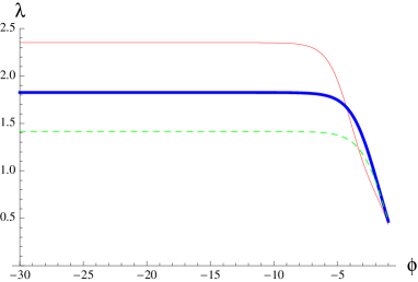
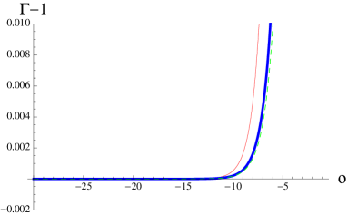
Figure 1: Plot of the function $\lambda(\phi)$ (left panel) and $\Gamma(\phi)-1$ (right panel) for selected values of the parameter $\beta$ representative of the three classes of solutions ($I,II$ and $III$) and for $w_{M}=0$. The thin, red lines are the plots relative to the model of class $I$ with $\beta=-15/64$. The thick blue lines give the plots of a model in class $II$ with $\beta=-1/8$. The green, dashed lines correspond to a model in class $III$ with $\beta=0$.

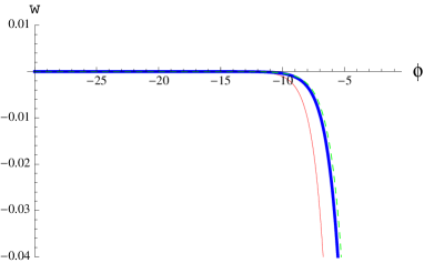
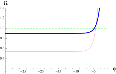
Figure 2: Plot of the function $w_{\phi}(\phi)$ (left panel) and $\Omega_{\phi}(\phi)$ (right panel) for selected values of the parameter $\beta$ representative of the three classes of solutions ($I,II$ and $III$) and for $w_{M}=0$. The thin, red lines are the plots relative to the model of class $I$ with $\beta=-15/64$. The thick blue lines give the plot of a model in class $II$ $\beta=-1/8$. The green, dashed lines correspond to a model in class $III$ with $\beta=0$.

Let us conclude this section with a brief, general discussion about the parameters entering in our model. Basically, apart from the Planck mass in the action (1) enter a dimensionless parameter $\beta$ and a length scale $R_{0}$ (Notice that in Eq. (1) we have set $\kappa^{2}=8\pi G=1/2$). In addition we have the integration constants of the differential equations (V), which have to be determined by solving the Cauchy problem. Some of these constants will be related to $t_{-}$ and $a,b$ characterizing respectively the power-law (29) and the exponential regime (44). However, the scale symmetries of the gravitational background together with the attractor behaviour of the scaling solution and of the de Sitter fixed point make the cosmological dynamics largely, if not completely, independent from the initial conditions. Cosmological evolution can be seen as a flow from a scaling fixed point to a conformal dS fixed point, in which the system looses any memory about initial conditions. The final state is therefore completely characterized by the length scale $R_{0}$, which determines everything (Hubble parameter, acceleration, cosmological constant and the mass for the scalar, see Eq. (30). The length scale $R_{0}$ can be fixed by the dark energy density necessary to explain the present acceleration of the universe, $\rho_{de}=10^{-123}m_{p}^{4}$. This gives a mass of the scalar $m\approx 10^{-33}eV$.

On one side this uniqueness gives a lot of predictive power to the model, but on the other side the presence of an extremely light scalar excitation runs into the the well-known problems in the framework of particle physics, SUGRA theories and cosmological constant scenarios Peebles and Ratra (2003); Padmanabhan (2003).

VI Conclusions

In this paper we have shown that scalar solitonic solutions of holographic models with hyperscaling violation have an interesting cosmological counterpart, which can be obtained by analytical continuation and by flipping the sign of the potential for the scalar field. The resulting flat FLRW solutions can be used to model cosmological evolution driven by dark energy and usual matter.

In absence of matter, the flow from the hyperscaling regime to the conformal AdS fixed point in holographic models correspond to cosmological evolution from power-law regime at early cosmic times to a dS fixed point at late times. In presence of matter, we have a scaling regime at early times, followed by an intermediate regime with tracking behaviour. At late times the solution exits the scaling regime with a sharp transition to a de Sitter spacetime. The phase transition between hyperscaling violation and conformal fixed point observed in holographic gravity has a cosmological analogue in the transition between a scaling, era and a dS era dominated by the energy of the vacuum.

We have been able to solve exactly the dynamics only in absence of matter. When matter is present we do not have full control of the global solutions. Nevertheless, by writing the cosmological equations as a dynamical system and by investigating three approximated regimes we have given strong evidence that the above picture is realized.

At the present stage our model for dark energy cannot be completely realistic. In the matter dominated epoch the ratio $\Omega_{\phi}/\Omega_{m}\approx 1$, so that we have a problem with nucleosynthesis. Moreover, the late-time cosmology shares the same problems of all cosmological constant scenarios. The vacuum energy is an unnaturally tiny free parameter of the model. The same is true for the mass of the scalar excitation associated to the quintessence field.

There are several open questions, which are worth to be investigated in order to support the above picture. One should derive the exact full phase space description of the dynamical system in presence of matter to check the correctness of our results. In particular, having full control on the phase space would give a precise description of the sharp transition between the scaling and the dS regime. This would also help us to shed light on the analogy between the cosmological transition and the hyperscaling violation/ AdS holographic phase transition.

Other key points that could improve our knowledge on the subject are: (1) Comparison between the cosmological dynamics and the RN group equations for the holographic gravity theory; (2) understanding of the analogy phase transition/cosmological transition in terms of the analytical continuation.