Magnetic response to applied electrostatic field in external magnetic field

Abstract

We show, within QED and other possible nonlinear theories, that a static charge localized in a finite domain of space becomes a magnetic dipole, if it is placed in an external (constant and homogeneous) magnetic field in the vacuum. The magnetic moment is quadratic in the charge, depends on its size and is parallel to the external field, provided the charge distribution is at least cylindrically symmetric. This magneto-electric effect is a nonlinear response of the magnetized vacuum to an applied electrostatic field. Referring to a simple example of a spherically-symmetric applied field, the nonlinearly induced current and its magnetic field are found explicitly throughout the space, the pattern of lines of force is depicted, both inside and outside the charge, which resembles that of a standard solenoid of classical magnetostatics.

1 Introduction

With the two recent papers [1], [2] we started a series of works aimed at studying quantum electrodynamics (QED) (as well as other nonlinear Abelian theories that may be historically traced back to [3]) under the conditions where the intrinsic nonlinearity of the theory shows itself not only as interaction of electromagnetic fields with a strong background, but also with themselves.

Manifestations of nonlinearity of the first type mentioned have been a focus of attention during many years since, perhaps, the pioneering works [4, 5] (see [6] and more recent papers [7, 8] for some reviews of the subsequent advances in that field). The strong background was served in the corresponding studies by the constant and homogeneous electromagnetic field (note, however, Ref. [9], where a certain inhomogeneity was introduced, and Ref. [10], where it was shown that a strong nonhomogeneous magnetic field is able to produce pairs of neutral fermions from the vacuum) and by the field of a plane wave (see the review of the laser-associated researches in [11]), because in these cases the influence of the background could be exactly taken into account for arbitrarily large value of their amplitude through the use of exact solutions of the Dirac equation available for such cases. The Dirac propagators for the virtual electrons and positrons in Feynman graphs for the vacuum polarization were the agents of interaction with the background field in the intermediate state.

In those works the varying electromagnetic fields are treated as small perturbations of the background, and only the effects linear in their amplitudes are taken into account, such as birefringence, photon capture by a magnetic field [12, 13], modification of the Coulomb law [14, 15, 16], magnetic shift of the critical charge value [17], – and even the positronium collapse [18] may be placed among effects of this class. The arena of applicability of these results is mostly the pulsars and magnetars, possessing sufficiently large magnetic fields.

In contrast with the above, in Refs. [1], [2] and in the present paper we are considering the effects, quadratic and cubic in the amplitude of the perturbation. As a matter of fact, two important  special examples of such effects were studied before, which were the processes of photon splitting in a magnetic [5, 19, 20, 21] and crossed [22] fields, and the light-by-light scattering  [23], all taken on the photon mass shell. Our goal is to deal with excitations of the vacuum, different from photons, subject to nonlinear version of the Maxwell equations, stemming from QED or, more generally, intrinsic to any other nonlinear electrodynamics. Whereas handling many-photon matrix elements beyond the photon mass shell, necessary for addressing a general nonlinear problem, turns out to be overcomplicated, we succeeded to indicate a simple approximation able to take responsibility for nonlinear effects in a universal manner and independent of an expansion in powers of the fine structure constant $\alpha,$ as far as QED is concerned. All kernels in the nonlinear integro-differential Maxwell equations are given in terms of variational field-derivatives of the effective action $\Gamma,$ defined as [24] the generating functional of irreducible vertices in QED, or as an action that fixes a theory in other versions of nonlinear electrodynamics. The approximation we are dealing with is referred to as the local or infrared approximation. It assumes that the effective action functional is local, i.e., it does not depend on the space-time derivatives of the field strength. True, this assumption restricts the range of applicability to only slow-varying fields in space and time, but it enables us to efficiently advance in describing the effects, cubic and quadratic in the field strength. By acting along these lines where there is no background  field [2], we reproduced the known [25, 23] correction to the Coulomb field which is cubic in the charge that produces it, and found cubic equations for dipole moments of selfinteracting fields of magnetic and electric dipoles that may be also viewed upon as nonlinear renormalizations of these quantities. In Ref. [1] we studied quadratic response of the background constant and homogeneous magnetic field to an applied electric field of a static charge at rest, and we found this response to be purely magnetic. In the present paper we continue the investigation of that magneto-electric effect, and we establish that the static charge placed into a background magnetic field is a magnetic dipole with its magnetic moment proportional to the charge squared and parallel to the background field, unless the charge distribution violates the initial cylindric symmetry of the problem. (This situation resembles our results [26] in noncommutative electrodynamics.) More explicit formulae for the magnetic field in the short and long ranges, for its lines of force and for the magnetic moment are presented referring to a simple example, where the applied electrostatic field is central-symmetric and would correspond, if in a nondispersive vacuum, to a charge distributed homogeneously inside a finite-radius sphere.

In the rest of the present Introduction we recall the basic equations of nonlinear electrodynamics, truncated at the third power of the varying field, against a constant homogeneous background, define the kernels in them as the second- and the third-rank polarization tensors in terms of the field-derivatives of the effective action, introduce nonlinearly-induced currents, and give expressions for the varying fields in terms of the currents based on the use of eigenvector expansion of the second-rank polarization tensor and the photon Green function. In Section 2 the second- and third-rank polarization tensors in a magnetic field are written in the infrared approximation as expressed in terms of the second and third derivatives of the delta-functions of the coordinate differences. The previously found linear-response correction to the Coulomb field of an arbitrarily distributed static charge at large distances in a magnetic field are given for completeness, and the general structure of quadratic response, which is purely magnetic, is analyzed in terms of eigenmodes contribution. In Section 3 very explicit expressions for the induced current and the magnetic field are fully elaborated using the simplest example, where the applied electric field is that of a homogeneously charged sphere of finite radius. Differential equations for the shape of the magnetic lines of force are solved, and the resulting pattern is drawn in Figs. 1 and 2 inside and outside the charge. The magnetic moment of the charge, proportional to its square, is given in terms of the background magnetic field and the radius of the charge. In Section 4 it is shown that spherically-nonsymmetric charge distributions also are characterized by a magnetic dipole moment, which is parallel to the background magnetic field, if the charge distribution does not specify any new direction in the space.

1.1 Nonlinear Maxwell equations

The exact electromagnetic field equations of QED with an external 4-current $j_{\mu}$ are the Euler-Lagrange equations $\frac{\delta S_{\mathrm{tot}}\left[A\right]}{\delta A^{\rho}(x)}=0$ that originate from the total action $S_{\mathrm{tot}}\left[A\right]$

$$S_{\mathrm{tot}}\left[A\right]=S_{\mathrm{Max}}\left[A\right]+\Gamma\left[A\right]+S_{\mathrm{int}}\left[A\right]\,,\ \ S_{\mathrm{Max}}\left[A\right]=-\int\mathfrak{F}\left(x\right)d^{4}x\,,$$ (1)

$$\Gamma\left[A\right]=\int\mathcal{L}\left(x\right)d^{4}x\,,\ \ S_{\mathrm{int}}\left[A\right]=-\int j_{\mu}\left(x\right)A^{\mu}\left(x\right)d^{4}x\,,\ \$$

$$\mathfrak{F}\left(x\right)=\frac{1}{4}F^{\mu\nu}F_{\mu\nu},\text{ }F^{\mu\nu}=\partial^{\mu}A^{\nu}(x)-\partial^{\nu}A^{\mu}(x),\text{ }\partial^{\mu}=\frac{\partial}{\partial x_{\mu}},$$

where $S_{\mathrm{Max}}\left[A\right]$ is the free Maxwell action, $\Gamma\left[A\right]$ is the effective action, and $\mathcal{L}\left(x\right)$ is the effective Lagrangian. Under the effective action $\Gamma$ we understand in QED the generating functional of one-particle-irreducible vertices [24]. Alternatively, it may be any action defining a nonlinear electrodynamics other than QED. Due to the gauge invariance it, as a matter of fact, depends only on the field strengths $F^{\mu\nu},$ and not of the 4-vector potentials $A^{\nu}.$ Besides, only the relativistic invariant combinations $\mathfrak{F}\left(z\right)=\frac{1}{4}F^{\mu\nu}F_{\mu\nu}$ and $\mathfrak{G}=\frac{1}{4}F^{\rho\sigma}\tilde{F}_{\rho\sigma}\mathbf{,}$ where the dual field tensor is defined as $\tilde{F}_{\rho\sigma}=\frac{1}{2}\epsilon_{\rho\sigma\lambda\kappa}F^{\lambda\kappa},$ of the field strengths make the arguments of $\Gamma$ and $\mathcal{L}$. In QED the effective action contains the exhausting and final information of the theory in the photon sector, and is subject to calculation within one or another dynamic scheme or approximation, especially the perturbation theory.

Expanding (1) in power series of the small electromagnetic field $a_{\mu}\left(x\right)=A_{\mu}(x)-\mathcal{A}_{\mu}(x)$ above the external background $\mathcal{A}(x)$ of a constant and homogeneous magnetic field $\mathbf{B=}$ $\left(\boldsymbol{\nabla}\times\boldsymbol{\mathcal{A}}\right)$, and restricting ourselves to the next-to-leading term, the minimum action condition becomes the nonlinear Maxwell equations:

$$\left[\square\eta_{\rho\nu}-\partial_{\rho}\partial_{\nu}\right]a^{\nu}\left(x\right)+\int d^{4}x^{\prime}\Pi_{\alpha\rho}\left(x^{\prime},x\right)a^{\alpha}\left(x^{\prime}\right)$$

$$+\frac{1}{2}\int d^{4}x^{\prime}d^{4}x^{\prime\prime}\Pi_{\alpha\beta\rho}\left(x^{\prime},x^{\prime\prime},x\right)a^{\alpha}\left(x^{\prime}\right)a^{\beta}\left(x^{\prime\prime}\right)=j_{\rho}\left(x\right)\,,$$ (2)

$$\Pi^{\alpha\rho}\left(x^{\prime},x\right)=\left.\frac{\delta^{2}\Gamma}{\delta A_{\alpha}\left(x^{\prime}\right)\delta A_{\rho}\left(x\right)}\right|_{A=\mathcal{A}}\,,$$

$$\Pi^{\alpha\beta\rho}\left(x^{\prime},x^{\prime\prime},x\right)=\left.\frac{\delta^{3}\Gamma}{\delta A_{\alpha}\left(x^{\prime}\right)\delta A_{\beta}\left(x^{\prime\prime}\right)\delta A_{\rho}\left(x\right)}\right|_{A=\mathcal{A}}\,,$$ (3)

where $\Pi^{\rho\alpha}\left(x^{\prime},x\right)$, $\Pi^{\alpha\beta\rho}\left(x^{\prime},x^{\prime\prime},x\right)$ are the second- and third-rank polarization tensor in an external magnetic field, respectively. Note that as long as the external field is constant in space-time, the polarization tensors (3) are functions on the differences of their arguments. In obtaining Eq. (2) the zero-order power of the field $a_{\mu}\left(x\right)$ does not appear, since the space-time-independent external field $\mathcal{F}^{\mu\nu}=\partial^{\mu}\mathcal{A}^{\nu}-\partial^{\nu}\mathcal{A}^{\mu}$ exactly obeys the sourceless Maxwell equations $\partial_{\mu}\mathcal{F}^{\mu\nu}=\left.\frac{\delta\Gamma}{\delta A_{\nu}\left(x\right)}\right|_{A=\mathcal{A}}=0$ . The power series has been truncated to the next-to-leading correction (i.e., we have neglected $\sim O\left(a^{3}\right)$).

Defining the nonlinear current as

$$j_{\rho}^{\mathrm{nl}}\left(x\right)=-\frac{1}{2}\int d^{4}x^{\prime}d^{4}x^{\prime\prime}\Pi_{\nu\sigma\rho}\left(x^{\prime},x^{\prime\prime},x\right)a^{\nu}\left(x^{\prime}\right)a^{\sigma}\left(x^{\prime\prime}\right)\,,\,$$ (4)

we may write (2) in the following way

$$\left[\square\eta_{\rho\nu}-\partial_{\rho}\partial_{\nu}\right]a^{\nu}\left(x\right)+\int d^{4}x^{\prime}\Pi_{\rho\alpha}\left(x^{\prime},x\right)a^{\alpha}\left(x^{\prime}\right)=j_{\rho}\left(x\right)+j_{\rho}^{\mathrm{nl}}\left(x\right)\,.$$ (5)

While solving the nonlinear set of Maxwell equations (5), (4) we should not, strictly speaking, exceed the initial accuracy. This implies that we treat the nonlinearity iteratively. To this end we divide its solution into two parts as $a_{\nu}(x)=a_{\nu}^{\text{{lin}}}(x)+a_{\nu}^{\text{{nl}}}(x),$ with $a_{\nu}^{\text{{lin}}}(x)\gg a_{\nu}^{\text{{nl}}}(x).$ Then, defining the linear field $a_{\nu}^{\text{{lin}}}(x)$ as a solution to the equation

$$\left[\square\eta_{\rho\nu}-\partial_{\rho}\partial_{\nu}\right]a_{\text{{lin}}}^{\nu}\left(x\right)+\int d^{4}x^{\prime}\Pi_{\rho\alpha}\left(x^{\prime},x\right)a^{\alpha}_{\text{{lin}}}\left(x^{\prime}\right)=j_{\rho}\left(x\right),$$ (6)

we get, as the first iteration, that the nonlinear correction $a_{\nu}^{\text{nl}}(x)$ to it is subject to the linear inhomogeneous equation

$$\left[\square\eta_{\rho\nu}-\partial_{\rho}\partial_{\nu}\right]a_{\mathrm{nl}}^{\nu}\left(x\right)+\int d^{4}x^{\prime}\Pi_{\rho\alpha}\left(x^{\prime},x\right)a_{\text{{nl}}}^{\alpha}\left(x^{\prime}\right)=\left.j_{\sigma}^{\text{nl}}\left(x^{\prime}\right)\right|_{a=a_{\text{lin}}}\,,$$ (7)

where

$$\left.j_{\rho}^{\text{nl}}\left(x^{\prime}\right)\right|_{a=a_{\text{lin}}}=-\frac{1}{2}\int d^{4}x^{\prime}d^{4}x^{\prime\prime}\Pi_{\rho\nu\sigma}\left(x^{\prime},x^{\prime\prime},x\right)a_{\text{{lin}}}^{\nu}\left(x^{\prime}\right)a_{\text{{lin}}}^{\sigma}\left(x^{\prime\prime}\right)$$ (8)

is the nonlinear current (4) taken at the linear value (9) of the field $a^{\nu}\left(x\right)=a_{\mathrm{lin}}^{\nu}\left(x\right).$The solution of Eqs. (6) and (7) may be written as

$$a_{\mathrm{lin}}^{\nu}\left(x\right) = \int d^{4}x^{\prime}D^{\nu\sigma}\left(x,x^{\prime}\right)j_{\sigma}\left(x^{\prime}\right)\,,$$ (9)

$$a_{\mathrm{nl}}^{\nu}\left(x\right) = \int d^{4}x^{\prime}D^{\nu\sigma}\left(x,x^{\prime}\right)\left.j_{\sigma}^{\text{nl}}\left(x^{\prime}\right)\right|_{a=a_{\text{lin}}},$$ (10)

The photon Green function in $D_{\mu\nu}(x,x^{\prime})$ above is defined as the inverse operator:

$$D_{\mu\nu}^{-1}(x-x^{\prime})=\left[\eta_{\mu\nu}\square-\partial_{\mu}\partial_{\nu}\right]\delta^{(4)}(x^{\prime}-x)+\Pi_{\mu\nu}(x-x^{\prime}).$$ (11)

Its Fourier transform $D^{\nu}{}_{\rho}(k)$ with respect to the coordinate difference should satisfy the following algebraic inhomogeneous equation

$$\left[k^{2}\eta_{\mu\nu}-k_{\mu}k_{\nu}-\Pi_{\mu\nu}(k)\right]D^{\nu}{}_{\rho}(k)=(\eta_{\mu\rho}-\frac{k_{\mu}k_{\rho}}{k^{2}}).$$ (12)

To solve this equation it is convenient to use the diagonal representation for the second-rank polarization operator in a magnetic field [27]

$$\Pi_{\mu\tau}(k,p)=\delta(k-p)\Pi_{\mu\tau}(k)\,,\ \ \Pi_{\mu\tau}(k)=\sum_{c=1}^{3}\varkappa_{c}(k)\frac{\flat_{\mu}^{(c)}\flat_{\tau}^{(c)}}{(\flat^{(c)})^{2}}$$ (13)

in terms of the mutually orthogonal 4-vectors $\flat_{\mu}^{(c)}$

$$\flat_{\mu}^{(1)}=(\mathcal{F}^{2}k)_{\mu}k^{2}-k_{\mu}(k\mathcal{F}^{2}k)\,,\ \ \flat_{\mu}^{(2)}=(\mathcal{\tilde{F}}k)_{\mu}\,,\ \ \flat_{\mu}^{(3)}=(\mathcal{F}k)_{\mu}\,,\ \ \flat_{\mu}^{(4)}=k_{\mu}\,,$$ (14)

where $(\mathcal{\tilde{F}}k)_{\mu}\equiv\mathcal{\tilde{F}}_{\mu\tau}k^{\tau}$, $(\mathcal{F}k)_{\mu}\equiv\mathcal{F}_{\mu\tau}k^{\tau}$, $(\mathcal{F}^{2}k)_{\mu}\equiv\mathcal{F}_{\mu\tau}^{2}k^{\tau}$, $k\mathcal{F}^{2}k\equiv k^{\mu}\mathcal{F}_{\mu\tau}^{2}k^{\tau}$, which are the eigenvectors of the polarization operator

$$\Pi_{\mu\tau}\flat^{(c)\tau}=\varkappa_{c}(k)\flat_{\mu}^{(c)},$$ (15)

the scalar functions $\varkappa_{c}(k)$ being its four eigenvalues, $\varkappa_{4}(k)=0$. The eigenvalues $\varkappa_{c}(k)$ depend on $\mathfrak{F}$ and on any two of the three momentum-containing Lorentz invariants $k^{2}=\mathbf{k}^{2}-k_{0}^{2},\;k\mathcal{F}^{2}k,\;k\mathcal{\tilde{F}}^{2}k$ , subject to one relation $\frac{k\mathcal{\tilde{F}}^{2}k}{2\mathfrak{F}}-k^{2}=\frac{k\mathcal{F}^{2}k}{2\mathfrak{F}}$, where $\mathfrak{F}$ is taken on the external field, $2\mathfrak{F=}$ $B^{2}.$ The solution of (12) has arbitrary longitudinal part:

$$D_{\mu\tau}(k) =\sum_{c=1}^{4}D^{(c)}(k)\frac{\flat_{\mu}^{(c)}\flat_{\tau}^{(c)}}{(\flat^{(c)})^{2}},$$

$$D^{(c)}(k) =\left\{\begin{tabular}[]{cc}$(k^{2}-\varkappa_{c}(k))^{-1},$&$c=1,2,3$\\ {arbitrary},&$c=4$\end{tabular}\,.\right.$$ (18)

It also has a diagonal form in the same terms as (13). This propagator has three components, corresponding to separate eigenmodes. Each of them has a pole in the 4-momentum plane, where solutions of the corresponding dispersion equations lie, i.e. on the photon mass shell, defined by the equations $k^{2}-\varkappa_{c}(k)=0$.

Now, solutions (9), (10) may be, respectively, written as

$$a_{\mu}^{\mathrm{lin}}(k) = \sum_{c=1}^{4}\frac{1}{(k^{2}-\varkappa_{c}(k))}\frac{\flat_{\mu}^{(c)}}{(\flat^{(c)})^{2}}(j^{\tau}\left(k\right)\flat_{\tau}^{(c)})\,,$$ (19)

$$a_{\mu}^{\mathrm{nl}}(k) = \sum_{c=1}^{4}\frac{1}{(k^{2}-\varkappa_{c}(k))}\frac{\flat_{\mu}^{(c)}}{(\flat^{(c)})^{2}}(j_{\mathrm{nl}}^{\tau}\left(k\right)\flat_{\tau}^{(c)})\,.$$ (20)

2 Response of magnetized vacuum to static electric field in the infrared approximation

In the rest of the paper we shall be treating equations of Subsection 2.1 in the low-momentum-low-frequency (infrared) approximation, $k_{\mu}\sim 0,$ which is stemming from the assumption that the effective action $\Gamma[A]$ is a local functional of the field strengths $F_{\mu\nu}$ in the sense that it does not contain their space- and time-derivatives. Examples of such action are the Heisenberg-Euler action available in the one-loop [23] and two-loop [28] approximations in QED, the Born-Infeld [29] action etc. Within the local limit the second- and third-rank polarization tensors (3) were calculated in [1] to give the result

$$\Pi_{\mu\nu}\left(x,x^{\prime}\right) = \left\{\mathcal{L}_{\mathfrak{F}}\left(\frac{\partial^{2}}{\partial x^{\mu}\partial x^{\nu}}-\eta_{\mu\nu}\square^{x}\right)\right.$$ (21)

$$- \left.\left(\mathcal{L}_{\mathfrak{FF}}\mathcal{F}_{\mu\alpha}\mathcal{F}_{\nu\beta}+\mathcal{L}_{\mathfrak{GG}}\mathcal{\tilde{F}}_{\mu\alpha}\mathcal{\tilde{F}}_{\nu\beta}\right)\frac{\partial^{2}}{\partial x_{\alpha}\partial x_{\beta}}\right\}\delta^{\left(4\right)}\left(x-x^{\prime}\right)\,,$$

$$\Pi_{\nu\rho\sigma}\left(x,x^{\prime},x^{\prime\prime}\right) = -\mathcal{O}_{\nu\rho\sigma\alpha\beta\gamma}\frac{\partial}{\partial x_{\alpha}}\left(\frac{\partial}{\partial x_{\beta}}\delta^{\left(4\right)}\left(x-x^{\prime}\right)\right)\left(\frac{\partial}{\partial x_{\gamma}}\delta^{\left(4\right)}\left(x^{\prime}-x^{\prime\prime}\right)\right)\,,$$ (22)

where

$$\mathcal{O}_{\mu\tau\sigma\alpha\beta\gamma}=\mathfrak{L_{GG}}\left[\widetilde{\mathcal{F}}_{\gamma\sigma}\epsilon_{\alpha\mu\beta\tau}+\widetilde{\mathcal{F}}_{\alpha\mu}\epsilon_{\beta\tau\gamma\sigma}+\widetilde{\mathcal{F}}_{\beta\tau}\epsilon_{\alpha\mu\gamma\sigma}\right]$$

$$+\mathfrak{L_{FF}}\left[\left(\eta_{\mu\tau}\eta_{\alpha\beta}-\eta_{\mu\beta}\eta_{\alpha\tau}\right)\mathcal{F}_{\gamma\sigma}+\mathcal{F}_{\alpha\mu}\left(\eta_{\tau\sigma}\eta_{\gamma\beta}-\eta_{\beta\sigma}\eta_{\gamma\tau}\right)+\mathcal{F}_{\beta\tau}\left(\eta_{\mu\sigma}\eta_{\gamma\alpha}-\eta_{\alpha\sigma}\eta_{\gamma\mu}\right)\right]$$

$$+\mathfrak{L_{FGG}}\left[{\mathcal{F}}_{\alpha\mu\text{ }}\widetilde{\mathcal{F}}_{\beta\tau}\widetilde{\mathcal{F}}_{\gamma\sigma}+\widetilde{\mathcal{F}}_{\alpha\mu}\mathcal{F}_{\beta\tau}\widetilde{\mathcal{F}}_{\gamma\sigma}\text{\emph{+}}\widetilde{\mathcal{F}}_{\alpha\mu}\widetilde{\mathcal{F}}_{\beta\tau}\mathcal{F}_{\gamma\sigma}\right]\text{ }+\mathfrak{L_{FFF}}\mathcal{F}_{\alpha\mu}\mathcal{F}_{\beta\tau}\mathcal{F_{\gamma\sigma}\,},$$ (23)

which expresses them in terms of the derivatives of the effective Lagrangian taken at the constant external field value, $\mathcal{F}^{\mu\nu}=\mathrm{const.}$,

$$\mathcal{L}\mathfrak{{}_{F}} =\left.\frac{d\mathcal{L}(\mathfrak{F},0))}{d\mathfrak{F}}\right|_{F=\mathcal{F}}\,,\ \ \mathcal{L}\mathfrak{{}_{FF}}=\left.\frac{d^{2}\mathcal{L}(\mathfrak{F},0)}{d\mathfrak{F}^{2}}\right|_{F=\mathcal{F}},\ \ \mathcal{L}\mathfrak{{}_{GG}}=\left.\frac{\partial^{2}\mathcal{L}(\mathfrak{F},\mathfrak{G})}{\partial\mathfrak{G}^{2}}\right|_{F=\mathcal{F},\mathfrak{G}=0}\,,$$ (24)

$$\mathcal{L}\mathfrak{{}_{FFF}} \mathfrak{=}\left.\frac{d^{3}\mathcal{L}(\mathfrak{F},0)}{d\mathfrak{F}^{3}}\right|_{F=\mathcal{F}}\,,\ \ \mathcal{L}\mathfrak{{}_{FGG}}=\frac{d}{d\mathfrak{F}}\left.\frac{\partial^{2}\mathcal{L}(\mathfrak{F},\mathfrak{G})}{\partial\mathfrak{G}^{2}}\right|_{F=\mathcal{F},\mathfrak{G}=0}\,.$$ (25)

It is taken into account that once the external field is purely magnetic in a certain Lorentz frame, the invariant $\mathfrak{G}$ for it is zero while $\mathfrak{F}$ is positive.

It was established in [30] that the second-rank polarization operator Eq. (21) has indeed the structure of (13) with the egenvalues $\varkappa_{a}(k)$ in the infrared regime being

$$\left.\varkappa_{1}(k^{2},k\mathcal{F}^{2}k,\mathfrak{F})\right|_{k\rightarrow 0} = k^{2}\mathcal{L}\mathfrak{{}_{F}},$$ (26)

$$\left.\varkappa_{2}(k^{2},k\mathcal{F}^{2}k,\mathfrak{F})\right|_{k\rightarrow 0} = k^{2}\mathcal{L}\mathfrak{{}_{F}}-(k\mathcal{\tilde{F}}^{2}k)\mathcal{L}\mathfrak{{}_{GG}},$$ (27)

$$\left.\varkappa_{3}(k^{2},k\mathcal{F}^{2}k,\mathfrak{F})\right|_{k\rightarrow 0} = k^{2}\mathcal{L}\mathfrak{{}_{F}}-(k\mathcal{F}^{2}k)\mathcal{L}\mathfrak{{}_{FF}}.$$ (28)

Hitherto, we shall be dealing only with sources that are static in a reference frame, where the external field is magnetic, i.e. time-independent charges at rest in a magnetic field

$$j_{\mu}(x)=\delta_{0\mu}q(\mathbf{x})\,,\ \ \text{$\tilde{j}$}_{\mu}(k)=(2\pi)\delta_{0\mu}\delta(k_{0})\tilde{q}(\mathbf{k}),$$ (29)

where the tilde marks the Fourier-transformed function.

2.1 Linear response – modified Coulomb law at large distances

Employing the source (29) in (19) and taking into account that at $k_{0}=0$ out of all the three (nontrivial) eigenvectors (14) only $\flat_{\mu}^{(2)}$ has its zeroth component different from zero, while its spatial components disappear $\flat_{i}^{(2)}=0,$ we get

$$a_{\text{{lin}}}^{0}(k)=(2\pi)\sum_{a=1}^{3}\frac{\delta(k_{0})\widetilde{q}(\mathbf{k})}{(k^{2}-\varkappa_{a}(k))}\frac{\flat_{0}^{(a)}}{(\flat^{(a)})^{2}}\flat_{0}^{(a)}=\frac{(2\pi)\delta(k_{0})\widetilde{q}(\mathbf{k})}{(\mathbf{k}^{2}-\varkappa_{2}(\mathbf{k}))}\,,\ \ \text{$\boldsymbol{a}$}_{\text{{lin}}}(k)=0\,.$$ (30)

(We disregarded the longitudinal part $k^{\mu}$ that does not contribute to the field strength). So, naturally, only static electric field is produced by a static source at the linear level (9), and no magnetic field.

Eq. (30) is approximation-independent. In the infrared limit, Eq. (27) is to be used in it with $k_{0}=0$ and $(k\tilde{F}^{2}k)=2\mathfrak{F}k_{3}^{2}=B^{2}k_{3}^{2}$ in the special frame, when the latter is so oriented that axis 3 coincide with the direction of the external magnetic field $\mathbf{B},$ $B=B_{3}=\mathcal{F}_{12},$ $B_{1,2}=0$. Then, in the coordinate space the linear potential (30) becomes

$$a_{\text{{lin}}}^{0}(\mathbf{x})=\frac{1}{(2\pi)^{3}}\int\frac{\widetilde{q}(\mathbf{k})e^{i\mathbf{k}_{\perp}\cdot\mathbf{x}_{\perp}}d^{2}k_{\perp}e^{ik_{3}\cdot x_{3}}dk_{3}}{\left(1-\mathcal{L}_{\mathfrak{F}}+2\mathfrak{F}\mathcal{L}_{\mathfrak{GG}}\right)k_{3}^{2}+\mathbf{k}_{\perp}^{2}\left(1-\mathcal{L}_{\mathfrak{F}}\right)}=\frac{1}{(2\pi)^{3}}\int\widetilde{q}(\mathbf{k})\frac{e^{i\mathbf{k}_{\perp}\cdot\mathbf{x}_{\perp}}d^{2}k_{\perp}e^{ik_{3}\cdot x_{3}}dk_{3}}{\varepsilon_{\text{{long}}}k_{3}^{2}+\mathbf{k}_{\perp}^{2}\varepsilon_{\text{{tr}}}}\,.$$ (31)

where we have used expressions for longitudinal and transverse dielectric constants from [30] (see also [31])

$$1-\mathcal{L}_{\mathfrak{F}}=\varepsilon_{\text{{tr}}},\text{ }1-\mathcal{L}_{\mathfrak{F}}+2\mathfrak{F}\mathcal{L}_{\mathfrak{GG}}=\varepsilon_{\text{{long}}}\,,$$

where the field invariant $\mathfrak{F}$ is henceforward taken on the external field, $2\mathfrak{F=}$ $B^{2},$ unlike its previous more general definition in (1). The subscript $\perp$ indicates projection onto (1, 2)-plane. The behavior of (31) at large distances $|\mathbf{x}_{\perp}|\rightarrow\infty,x_{3}\rightarrow\infty$ is

$$a_{\text{{lin}}}^{0}(\mathbf{x})\sim\frac{Q}{(2\pi)^{3}}\int\frac{e^{i\mathbf{k}_{\perp}\cdot\mathbf{x}_{\perp}}d^{2}k_{\perp}e^{ik_{3}\cdot x_{3}}dk_{3}}{\varepsilon_{\text{{long}}}k_{3}^{2}+\mathbf{k}_{\perp}^{2}\varepsilon_{\text{{tr}}}}\,,$$ (32)

where $Q=\widetilde{q}(0)=\int q(\mathbf{x)}d^{3}x$ is the total charge in understanding that the charge density is either compactly distributed inside a volume or decreases sufficiently fast outside it so that this integral converge.

By making the change of variables $\varepsilon_{\text{{long}}}^{1/2}k_{3}=k_{3}^{\prime},$ $\mathbf{k}_{\perp}\varepsilon_{\text{{tr}}}^{1/2}=\mathbf{k}_{\perp}^{\prime}$ the integral (32) is transformed to

$$a_{\text{{lin}}}^{0}(\mathbf{x}) \sim \frac{Q}{(2\pi)^{3}\varepsilon_{\text{{long}}}^{1/2}\varepsilon_{\text{{tr}}}}\int\frac{e^{i\mathbf{k}^{\prime}\cdot\mathbf{x}^{\prime}}d^{3}k^{\prime}}{\mathbf{k}^{\prime 2}}=\frac{Q}{4\pi\varepsilon_{\text{{long}}}^{1/2}\varepsilon_{\text{{tr}}}}\frac{1}{|\mathbf{x}^{\prime}|}$$ (33)

$$= \frac{1}{4\pi\varepsilon_{\text{{long}}}^{1/2}\varepsilon_{\text{{tr}}}}\frac{Q}{\left(\mathbf{x}_{\perp}^{2}\varepsilon_{\text{{tr}}}^{-1}+x_{3}^{2}\varepsilon_{\text{{long}}}^{-1}\right)^{1/2}}=\frac{1}{4\pi\varepsilon_{\text{{tr}}}^{1/2}}\frac{Q}{\left(\mathbf{x}_{\perp}^{2}\varepsilon_{\text{{long}}}+x_{3}^{2}\varepsilon_{\text{{tr}}}\right)^{1/2}},$$

where the notations $\mathbf{x}_{\perp}^{\prime}=\mathbf{x}_{\perp}\varepsilon_{\text{{tr}}}^{-1/2},$ $x_{3}^{\prime}=x_{3}\varepsilon_{\text{{long} }}^{-1/2}$ , $|\mathbf{x}^{\prime}|=(|\mathbf{x}_{\perp}^{\prime}|^{2}+(x_{3}^{\prime})^{2})^{1/2}$ were used. This anisotropic Coulomb law, resulted from the infrared limit (21) of the second-rank polarization operator, is thereby the long-distance asymptotic behavior of the electrostatic potential produced by a charge, locally distributed in space, in a constant magnetic field.

It may be also useful  to write the scalar potential (33) in an O(3)-invariant way as a function of two rotational scalars:

$$a_{\text{{lin}}}^{0}(\mathbf{x})=a_{\text{{lin}}}^{0}(\mathbf{x}^{2},(\mathbf{B\cdot x}))=\frac{1}{4\pi\varepsilon_{\text{{tr}}}^{1/2}}\frac{Q}{\left(\mathbf{x}^{2}\varepsilon_{\text{{long}}}+(\mathbf{B\cdot x})^{2}\mathcal{L}_{\mathfrak{GG}}\right)^{1/2}}.$$ (34)

Previously [14, 15], that potential was found in QED in the whole space, the vicinity of the charge – where the potential has the Debye form – included,  starting from the off-shell calculations of the full (free of the restrictive assumption $k_{\mu}$ $\sim 0)$ second-rank off-shell polarization operator in a magnetic field, first performed within the accuracy of one fermion loop in [27]. If the one-loop Heisenberg-Euler effective Lagrangian is taken for $\mathcal{L}$ in (33), it makes (a corrected form of) the large-distance behavior of the potential in QED.

2.2 Quadratic response – magneto-electric effect

When the four-vector potential in expression (4) is chosen as $a^{\mu}\left(\mathbf{x}\right)\simeq a_{\text{lin}}^{\mu}\left(\mathbf{x}\right)=\delta_{0\mu}$ $a_{\text{lin}}^{0}\left(\mathbf{x}\right),$ so as to carry only electrostatic field $\mathbf{E\left(\mathbf{x}\right)=}-\mathbf{\nabla}a^{0}\left(\mathbf{x}\right),$ the nonlinear current (4), approximated as (8) in accord with the iteration (7), (henceforth we omit the explicit indication that it is taken on linear fields), becomes [1], up to the third and fourth powers of the applied field

$$j_{\mathrm{nl}}^{0}\left(\mathbf{x}\right)=0\,,\ \ \mathbf{j}_{\mathrm{nl}}\left(\mathbf{x}\right)=\mathbf{j}_{\mathfrak{FF}}\left(\mathbf{x}\right)+\mathbf{j}_{\mathfrak{FGG}}\left(\mathbf{x}\right)+\mathbf{j}_{\mathfrak{GG}}\left(\mathbf{x}\right)\,,$$ (35)

$$\mathbf{j}_{\mathfrak{FF}}\left(\mathbf{x}\right)=\frac{\mathcal{L}_{\mathfrak{FF}}}{2}\left(\boldsymbol{\nabla}\times\mathbf{B}\right)\mathbf{E}^{2}\,,\ \ \mathbf{j}_{\mathfrak{FGG}}\left(\mathbf{x}\right)=-\frac{\mathcal{L}_{\mathfrak{FGG}}}{2}\left(\boldsymbol{\nabla}\times\mathbf{B}\right)\left(\mathbf{B}\cdot\mathbf{E}\right)^{2}\,,$$

$$\mathbf{j}_{\mathfrak{GG}}\left(\mathbf{x}\right)=-\mathcal{L}_{\mathfrak{GG}}\left(\boldsymbol{\nabla}\times\mathbf{E}\right)\left(\mathbf{B}\cdot\mathbf{E}\right)\,,$$

after the expression (22) for the third-rank polarization tensor in the local limit is used. Here every derivative acts on everything to the right of it.

Note that in (35), $\mathbf{E}$ is the applied electric field, the nonlinear response to which is under consideration. Correspondingly, Eq. (35) is quadratic with respect to $\mathbf{E.}$ On the contrary, the external magnetic field $\mathbf{B=}$ $\left(\boldsymbol{\nabla}\times\boldsymbol{\mathcal{A}}\right),$ $B$ $=\left(2\mathfrak{F}\right)^{1/2\text{ }}$ enters (35) with all powers, since the coefficients in it depend on $B$ in a complicated way according to their definitions (24) and (25).

Let us discuss the structure of the nonlinear correction to the electromagnetic field caused by the current (35) following Eq. (10). We appeal to representation (18) for the photon propagator in it. First we note that the mode $c=2$ does not contribute, since $j_{\mathrm{nl}}^{0}=0,$ and $\flat_{i}^{(2)}=(\mathcal{\tilde{F}}k)_{i}$ (14) disappears, when multiplied by the Fourier transform $\mathbf{\widetilde{\mathbf{j}}}_{\mathrm{nl}}\left(\mathbf{k}\right)\delta(k_{0})$ of (35). Also the zeroth components of the other two eigenvectors (14) $\flat_{0}^{(1,3)}$ vanish if taken at $k_{0}=0$. Thus we are left with,

$$a_{\mathrm{nl}}^{0}=0\,,\ \ a_{\text{{nl}}}^{i}(k)=\sum_{c=1,3}\frac{(2\pi)\delta(k_{0})}{(k^{2}-\varkappa_{c}(k))}\frac{\flat_{i}^{(c)}}{(\flat^{(c)})^{2}}(\widetilde{j}_{j\mathrm{nl}}\left(\mathbf{k}\right)\flat_{j}^{(c)})\,,$$ (36)

which indicates that the quadratic response to a static electric field is purely magnetic.

It can be shown that Eqs. (36) are in fact exact relations in the electrostatic case independent of the infrared approximation. This implies that in that instance only modes 1 and 3 propagate magnetic field. However, in a spherically symmetric infrared example to be considered below it holds that $\widetilde{j}_{j\mathrm{nl}}\left(\mathbf{k}\right)\flat_{j}^{(1)}=0,$ so only the term $c=3$ contributes in the nonlinear electromagnetic field (36).

If the linear vacuum polarization (in fact, the magnetization) is neglected, $\varkappa_{1,3}=0,$ the nonlinear magnetic field $\mathbf{h}=\mathbf{k}\times\boldsymbol{a}_{\text{nl}}$ obtained from (36) satisfies the standard Maxwell equation $\mathbf{k}^{2}\boldsymbol{a}_{\text{nl}}=\mathbf{\widetilde{\mathbf{j}}}_{\mathrm{nl}}$. In this case this field follows from (35) to be [1],

$$h_{i}\left(\mathbf{x}\right)=\mathfrak{h}_{i}\left(\mathbf{x}\right)+\frac{\partial_{i}\partial_{k}}{4\pi}\mathfrak{I}_{k}\left(\mathbf{x}\right)\,,\ \ \mathfrak{I}_{k}\left(\mathbf{x}\right)=\int d^{3}y\frac{\mathfrak{h}_{k}\left(\mathbf{y}\right)}{\left|\mathbf{x}-\mathbf{y}\right|}\,,$$ (37)

where

$$\mathfrak{h}_{i}\left(\mathbf{x}\right)=\mathfrak{h}_{i}^{\mathfrak{FF}}\left(\mathbf{x}\right)+\mathfrak{h}_{i}^{\mathfrak{FGG}}\left(\mathbf{x}\right)+\mathfrak{h}_{i}^{\mathfrak{GG}}\left(\mathbf{x}\right)\,,$$

$$\mathfrak{h}_{i}^{\mathfrak{FF}}=\frac{B_{i}}{2}\mathcal{L}_{\mathfrak{FF}}\mathbf{E}^{2}\,,\ \mathfrak{h}_{i}^{\mathfrak{FGG}}=-\frac{B_{i}}{2}\mathcal{L}_{\mathfrak{FGG}}\left(\mathbf{B}\cdot\mathbf{E}\right)^{2}\,,\ \ \mathfrak{h}_{i}^{\mathfrak{GG}}=-\mathcal{L}_{\mathfrak{GG}}\left(\mathbf{B}\cdot\mathbf{E}\right)E_{i}\,.$$ (38)

3 Quadratic magnetic response to a spherically-symmetric applied electric field. Simple example

In this Section, in order to present the magneto-electric effect in its most explicit way, we shall consider the magnetic field, which is the response of the vacuum to the applied electric field, whose vector potential is chosen to be the following smooth spheric-symmetrical Coulomb-like function

$$a_{0}\left(r\right)=a_{0}^{\mathrm{I}}\left(r\right)\theta\left(R-r\right)+a_{0}^{\mathrm{II}}\left(r\right)\theta\left(r-R\right)\,,\,\,r=\left|\mathbf{x}\right|$$ (39)

$$a_{0}^{\mathrm{I}}\left(r\right)=-\frac{Ze}{8\pi R^{3}}r^{2}+\frac{3Ze}{8\pi R}\,,\ \ a_{0}^{\mathrm{II}}\left(r\right)=\frac{Ze}{4\pi r}\,.$$

Here $\theta\left(z\right)$ is the Heaviside unit step function, defined as

$$\theta\left(z\right)=\left\{\begin{array}[]{c}1\,,\ \ z>0\,,\\ 1/2\,,\ \ z=0\,,\\ 0\,,\ \ z<0\,.\end{array}\right.\,,\ \ \frac{d}{dz}\theta\left(z\right)=\delta\left(z\right)\,,$$

and $\delta\left(z\right)$ stands for the Dirac delta function. Eq. (39) supplies us with the simplest example, where the magnetic field comprising the nonlinear vacuum respond can be explicitly studied, the shape of the lines of force being fully described. If not for the linear polarization, the potential (39) would be the field of extended spherically-symmetric charge

distributed with the constant density $\rho\left(r\right)$ inside a sphere $r\leq R$ with the radius $R$:

$$\rho\left(r\right)=\left(\frac{3}{4\pi}\frac{Ze}{R^{3}}\right)\theta\left(r-R\right)\,.$$ (40)

However, it should be kept in mind that with the account of the linear vacuum polarization, the potential distribution (39) cannot be supported by any spherically-symmetric charge, strictly localized in a finite space domain. To find the genuine source of the field (39), one should apply the operator in the left-hand side of (6) to it. The result looks like:

$$\rho_{\text{lin}}\left(\mathbf{x}\right)=\rho\left(r\right)(1-\mathcal{L}_{\mathfrak{F}})+2\mathfrak{F}\mathcal{L}_{\mathfrak{GG}}\left(1+\frac{(\mathbf{B\cdot x})^{2}}{B^{2}}\frac{d}{rdr}\right)\frac{d}{rdr}a_{0}\left(r\right).$$

This charge density is cylindrically symmetric and extends beyond the sphere, $r>R,$ decreasing as 1/$r^{3},$ or 1/$x_{3}^{3}$ far from it, depending on the direction.

In the next Section the particular result to be formulated in the present Section that the magnetic response to an electrostatic field implies that the charge giving rise to the latter carries a magnetic dipole moment parallel to the external magnetic field will be confirmed for a general charge density distribution and for its, cylindrically-symmetric in the remote domain, electrostatic field, where the linear response is also included. Only the expression for the magnetic moment will be less explicit, as well as expressions for the induced magnetic field and the shape of its lines of force in the region closer to the charge. The aim of the present Section is just to detail these appealing to the simplified example of (39).

Now we proceed with the applied potential (39). It provides the following electric field

$$\mathbf{E}\left(\mathbf{x}\right)=\left(\frac{Ze}{4\pi}\right)\mathcal{E}\left(r\right)\mathbf{x}\,,$$ (41)

$$\mathcal{E}\left(r\right)=\frac{\theta\left(R-r\right)}{R^{3}}+\frac{\theta\left(r-R\right)}{r^{3}}\,.$$ (42)

In writing the expression for (42) we took into account the continuity of (39) and of its derivatives at $r=R$.  As a result, Dirac-delta terms stemming from the differentiation of the step function could be omitted (see Appendix for a general discussion on the subject). This simplification will be used every time functions are continuous.

3.1 Nonlinearly induced current

Taking into account the electric field (41) and

$$\mathcal{E}^{2}\left(r\right)=\frac{\theta\left(R-r\right)}{R^{6}}+\frac{\theta\left(r-R\right)}{r^{6}}\,,$$ (43)

contributions (35) into the nonlinear current take the form,

$$j_{i}^{{}_{\mathfrak{FF}}}\left(\mathbf{x}\right)=\mathcal{L}_{\mathfrak{FF}}\varepsilon_{ijk}B_{k}E_{l}\partial_{j}E_{l}\,,$$

$$j_{i}^{{}_{\mathfrak{FGG}}}\left(\mathbf{x}\right)=-\mathcal{L}_{\mathfrak{FGG}}\varepsilon_{ijk}B_{k}B_{l}B_{n}E_{l}\left(\partial_{j}E_{n}\right)\,,$$

$$j_{i}^{\mathfrak{GG}}\left(\mathbf{x}\right)=-\mathcal{L}_{\mathfrak{GG}}\varepsilon_{ijk}\partial_{j}\left(E_{k}B_{l}E_{l}\right).$$ (44)

Therefore

$$\mathbf{j}_{\mathrm{nl}}\left(\mathbf{x}\right) = \left(\frac{Ze}{4\pi}\right)^{2}\left\{\left(\mathcal{L}_{\mathfrak{FF}}+\mathcal{L}_{\mathfrak{GG}}\right)\frac{\theta\left(R-r\right)}{R^{6}}\right.$$ (45)

$$+ \left.\left(\mathcal{L}_{\mathfrak{GG}}-2\mathcal{L}_{\mathfrak{FF}}+3\mathcal{L}_{\mathfrak{FGG}}\frac{\left(\mathbf{B}\cdot\mathbf{x}\right)^{2}}{r^{2}}\right)\frac{\theta\left(r-R\right)}{r^{6}}\right\}\left(\mathbf{x\times B}\right)\,.$$

Again, thanks to the continuity of $\mathbf{E}\left(\mathbf{x}\right)$ (41), expressions (44), (45) do not contain the $\delta$-like contributions that might come from the differentiation of the Heaviside $\theta$-function. But the nonlinear current is discontinuous at the surface of the sphere $r=R$. We shall see below that the magnetic field produced by it is still continuous.

The lines of the nonlinear current (45) are circular and lie in planes, orthogonal to the external magnetic field. Its density decreases as the sixth power of the distance from the center of the charge, or of the distance from the axis, parallel to the external magnetic field – for large distances.

Eq. (45) is our final expression for the current that may be of independent interest. In calculating the magnetic field produced by it in the next Subsection, however, we shall not exploit it, but refer to expressions of the previous Sections.

Observe that the proportionality of the current $\mathbf{j}_{\mathrm{nl}}\left(\mathbf{x}\right)$ above to $\left(\mathbf{x\times B}\right),$ and hence its circular character in the transverse plane, is valid also for any spherically-symmetric field distribution like (41), irrespective of the special form (42). This property means that an expansion of (35) over the (spacial part of) eigenvectors of the polarization operator in a magnetic field (14) does not contain, in the momentum space, a nonvanishing contribution proportional to the vector $\mathbf{b}^{(1)},$ whose components are  $\flat_{1,2}^{(1)}=k_{1,2}k_{3}^{2},$ $\flat_{3}^{(1)}=-k_{3}(k_{1}^{2}+k_{2}^{2}),$ but is proportional to the vector $\mathbf{b}^{(3)},$ such that $\flat_{3}^{(3)}=0,$ $\flat_{1}^{(3)}=-k_{2},$ $\flat_{2}^{(3)}=k_{1},$ which is thereby the only vector contributing in the expansion of the nonlinear current in spherically-symmetric case. [The three vectors $\mathbf{b}^{(1)},\ \mathbf{b}^{(3)},$and $\mathbf{b}^{(4)}=\mathbf{k}$ are mutually orthogonal. There is no contribution proportional to $\mathbf{b}^{(4)}$ due to the continuity $\mathbf{\nabla j}_{\text{{nl}}}=0.$ As for the eigenvector $\flat_{\mu}^{(2)},$ its spacial part is zero in our static case of $k_{0}=0.$] Correspondingly, only the value $c=3$ appears in the expansion of the nonlinear magnetic field (36). We do not know, if this circumstance may be a general consequence of the spherical symmetry, independent of the infrared approximation.

3.2 Nonlinearly induced magnetic field

We shall calculate here the magnetic field, nonlinearly induced by the electrostatic field (39) within the infrared approximation, basing on Eq. (37), which assumes the neglect of the linear vacuum polarization.

3.2.1 Second contribution in (37)

In order to find the integrals $\mathfrak{I}_{k}\left(\mathbf{x}\right)=\mathfrak{I}_{k}^{\mathfrak{FF}}\left(r\right)+\mathfrak{I}_{k}^{\mathfrak{FGG}}\left(\mathbf{x}\right)+\mathfrak{I}_{k}^{\mathfrak{GG}}\left(\mathbf{x}\right)$ it should be noted that the three their parts have the following structure:

$$\mathfrak{I}_{k}^{\mathfrak{FF}}\left(r\right)=\int d^{3}y\frac{\mathfrak{h}_{k}^{\mathfrak{FF}}\left(y\right)}{\left|\mathbf{x}-\mathbf{y}\right|}=\frac{1}{2}\left(\frac{Ze}{4\pi}\right)^{2}\mathcal{L}_{\mathfrak{FF}}B_{k}v\left(r\right)\,,\,\,y=\left|\mathbf{y}\right|\,,$$

$$\mathfrak{I}_{k}^{\mathfrak{FGG}}\left(\mathbf{x}\right)=\int d^{3}y\frac{\mathfrak{h}_{k}^{\mathfrak{FGG}}\left(\mathbf{y}\right)}{\left|\mathbf{x}-\mathbf{y}\right|}=-\frac{1}{2}\left(\frac{Ze}{4\pi}\right)^{2}\mathcal{L}_{\mathfrak{FGG}}B_{k}\left[(\mathbf{B\cdot x)}^{2}u(r)+B^{2}w(r)\right]\,,$$

$$\mathfrak{I}_{k}^{\mathfrak{GG}}\left(\mathbf{x}\right)=\int d^{3}y\frac{\mathfrak{h}_{k}^{\mathfrak{GG}}\left(\mathbf{y}\right)}{\left|\mathbf{x}-\mathbf{y}\right|}=-\left(\frac{Ze}{4\pi}\right)^{2}\mathcal{L}_{\mathfrak{GG}}\left[x_{k}(\mathbf{B\cdot x)}u(r)+B_{k}w(r)\right]\,,$$ (46)

where

$$v\left(r\right)=\int d^{3}y\frac{\mathcal{E}^{2}\left(y\right)y^{2}}{\left|\mathbf{x}-\mathbf{y}\right|}\,,$$ (47)

and $u(r)$ and $w(r)$ are the scalar coefficients in the tensor decomposition

$$\int d^{3}y\frac{\mathcal{E}^{2}\left(y\right)y_{i}y_{k}}{\left|\mathbf{x}-\mathbf{y}\right|}=u\left(r\right)x_{i}x_{j}+w\left(r\right)\delta_{ij}\,.$$ (48)

The basic angular integrals involved in (47), (48) are (we refer to Eq. (2.222) in [33] for their values):

$$V_{1}(r,y)=\int_{-1}^{1}d\left(\cos\vartheta\right)\frac{1}{\sqrt{r^{2}+y^{2}-2ry\cos\vartheta}}=\frac{1}{ry}\left\{r+y-\left|r-y\right|\right\}\,,\text{ \ }r,y\geqslant 0\,,$$ (49)

and

$$V_{2}(r,y) = \int_{-1}^{1}d\left(\cos\vartheta\right)\frac{\cos^{2}\vartheta}{\sqrt{r^{2}+y^{2}-2ry\cos\vartheta}}$$ (50)

$$= \left(\frac{2r^{4}-2r^{3}y+7r^{2}y^{2}-2ry^{3}+2y^{4}}{15r^{3}y^{3}}\right)(r+y)$$

$$- \left(\frac{2r^{4}+2r^{3}y+7r^{2}y^{2}+2ry^{3}+2y^{4}}{15r^{3}y^{3}}\right)\left|r-y\right|\,,\text{ \ }r,y\geqslant 0\,.$$

One can immediately verify that $v\left(r\right)$ (47) takes the form

$$v\left(r\right)=2\pi\int_{0}^{\infty}dyy^{4}\mathcal{E}^{2}\left(y\right)V_{1}(r,y)\,.$$ (51)

Further, once (48) does not depend on $\mathbf{B}$, one can choose $\mathbf{B\perp x}$ to find,

$$w(r)=\frac{1}{\mathbf{B}^{2}}\int d^{3}y\left.\frac{\mathcal{E}^{2}\left(y\right)(\mathbf{B\cdot y)}^{2}}{\left|\mathbf{x}-\mathbf{y}\right|}\right|_{{}_{\mathbf{B\perp x}}}=\pi\int_{0}^{\infty}dy\mathcal{E}^{2}\left(y\right)\left(V_{1}(r,y)-V_{2}(r,y)\right)\,.$$ (52)

When getting this result we counted off the angle $\vartheta$ from the radius-vector $\mathbf{x,}$ and $\varphi$ from $\mathbf{B}$, so that $\mathbf{B\cdot y}=By\sin\vartheta\cos\varphi$, and took into account the relation $\int_{0}^{2\pi}\cos^{2}\varphi d\varphi=\pi$. Analogously, by choosing $\mathbf{B\parallel x}$ we find from (48) that

$$r^{2}u\left(r\right)+w\left(r\right) = \frac{1}{\mathbf{B}^{2}}\int d^{3}y\left.\frac{\mathcal{E}^{2}\left(y\right)(\mathbf{B\cdot y)}^{2}}{\left|\mathbf{x}-\mathbf{y}\right|}\right|_{{}_{\mathbf{B\parallel x}}}$$

$$= 2\pi\int_{0}^{\infty}dyy^{4}\mathcal{E}^{2}\left(y\right)V_{2}(r,y)\,,$$

since now $\mathbf{B\cdot y=}By\cos\vartheta.$ Using Eq. (52) for $w\left(r\right)$ we get the function $u\left(r\right)$ in (48),

$$u(r)=\frac{\pi}{r^{2}}\int_{0}^{\infty}dyy^{4}\mathcal{E}^{2}\left(y\right)\left(3V_{2}(r,y)-V_{1}(r,y)\right)\,.$$ (54)

Now Eqs. (51), (52), and (54) define the contributions (46) into the field $\mathbf{h}\left(\mathbf{x}\right)$ according to (37). These equations are valid, generally, for arbitrary spherically symmetric field distribution of the form (41), provided that $\mathcal{E}\left(r\right)$ there decreases sufficiently fast at large $r$ to guarantee the convergence of the remaining integrals over $y$. For $\mathcal{E}^{2}\left(y\right)$ taken as (43) the remaining $y$-integrations in (51) and (3.2.1) can be explicitly done with the help of (49), (50), and their calculation is illustrated in Appendix.

We obtain in this way

$$v\left(r\right)=\pi\left[\frac{3}{R^{2}}\left(1-\frac{r^{4}}{15R^{4}}\right)\theta\left(R-r\right)+\frac{2}{r^{2}}\left(\frac{12r}{5R}-1\right)\theta\left(r-R\right)\right]\,,$$ (55)

for (51), and

$$r^{2}u\left(r\right)+w\left(r\right) = \frac{\pi}{R^{2}}\left(1+\frac{2r^{2}}{5R^{2}}-\frac{9r^{4}}{35R^{4}}\right)\theta\left(R-r\right)$$

$$+ \frac{8\pi}{5Rr}\left(1-\frac{2R^{2}}{7r^{2}}\right)\theta\left(r-R\right)\,,$$

$$u\left(r\right) = \frac{3\pi}{5R^{2}}\left(1-\frac{10r^{2}}{21R^{2}}\right)\frac{\theta\left(R-r\right)}{R^{2}}+\pi\left(1-\frac{24R}{35r}\right)\frac{\theta\left(r-R\right)}{r^{4}}\,,$$

$$w\left(r\right) = \pi\left(1-\frac{r^{2}}{5R^{2}}+\frac{r^{4}}{35R^{4}}\right)\frac{\theta\left(R-r\right)}{R^{2}}$$ (56)

$$- \pi\left(1-\frac{8r}{5R}-\frac{8R}{35r}\right)\frac{\theta\left(r-R\right)}{r^{2}}$$

for (3.2.1), (54) and (52). With these results the integrals (46) have the form

$$\mathfrak{I}_{k}^{\mathfrak{FF}}\left(r\right)=\pi\left(\frac{Ze}{4\pi}\right)^{2}\mathcal{L}_{\mathfrak{FF}}B_{k}\left[\mathcal{I}_{1}\left(r\right)\theta\left(R-r\right)+\mathcal{I}_{2}\left(r\right)\theta\left(r-R\right)\right]\,,$$ (57)

$$\mathfrak{I}_{k}^{\mathfrak{FGG}}\left(\mathbf{x}\right)=\pi\left(\frac{Ze}{4\pi}\right)^{2}\mathcal{L}_{\mathfrak{FGG}}B_{k}\left[\mathcal{I}_{3}\left(r\right)\theta\left(R-r\right)+\mathcal{I}_{4}\left(r\right)\theta\left(r-R\right)\right]\,,$$ (58)

$$\mathfrak{I}_{k}^{\mathfrak{GG}}\left(\mathbf{r}\right)=\pi\left(\frac{Ze}{4\pi}\right)^{2}\mathcal{L}_{\mathfrak{GG}}\left[\mathcal{I}_{k}^{5}\left(r\right)\theta\left(R-r\right)+\mathcal{I}_{k}^{6}\left(r\right)\theta\left(r-R\right)\right]\,,$$ (59)

where

$$\mathcal{I}_{1}\left(r\right) = \frac{3}{2R^{2}}\left(1-\frac{r^{4}}{15R^{4}}\right)\,,\ \ \mathcal{I}_{2}\left(r\right)=-\frac{1}{r^{2}}\left(1-\frac{12r}{5R}\right)\,,$$

$$\mathcal{I}_{3}\left(r\right) = -\frac{1}{2R^{2}}\left[\left(1-\frac{r^{2}}{5R^{2}}+\frac{r^{4}}{35R^{4}}\right)B^{2}+\frac{3r^{2}}{5R^{2}}\left(1-\frac{10r^{2}}{21R^{2}}\right)\left(\frac{\mathbf{B\cdot x}}{r}\right)^{2}\right]\,,$$

$$\mathcal{I}_{4}\left(r\right) = -\frac{4}{5Rr}\left[\left(1+\frac{R^{2}}{7r^{2}}-\frac{5R}{8r}\right)B^{2}+\frac{5R}{8r}\left(1-\frac{24R}{35r}\right)\left(\frac{\mathbf{B\cdot x}}{r}\right)^{2}\right]\,,$$

$$\mathcal{I}_{k}^{5}\left(r\right) = -\frac{3x_{k}(\mathbf{B\cdot x)}}{5R^{4}}\left(1-\frac{10r^{2}}{21R^{2}}\right)-\frac{B_{k}}{R^{2}}\left(1-\frac{r^{2}}{5R^{2}}+\frac{r^{4}}{35R^{4}}\right)\,,$$

$$\mathcal{I}_{k}^{6}\left(r\right) = -\frac{x_{k}(\mathbf{B\cdot x)}}{r^{4}}\left(1-\frac{24R}{35r}\right)+\frac{B_{k}}{r^{2}}\left(1-\frac{8r}{5R}-\frac{8R}{35r}\right)\,.$$ (60)

Using these representations it is straightforward to make sure that the functions (57) – (59) are continuous in the point $r=R$. So are also all their first and second derivatives with respect to the coordinate components. Consequently, the Dirac delta-functions and their derivatives, which stem from differentiation of the step-functions in the calculation of $\partial_{i}\partial_{k}\mathfrak{I}_{k}\left(\mathbf{x}\right)/4\pi$ from (46), do not contribute (see Appendix). As a result these derivatives can be left in their simplest form,

$$\frac{\partial_{i}\partial_{k}}{4\pi}\mathfrak{I}_{k}\left(\mathbf{x}\right) = \left(\frac{Ze}{8\pi}\right)^{2}\left\{\partial_{i}\partial_{k}\left[\mathcal{L}_{\mathfrak{FF}}B_{k}\mathcal{I}_{1}\left(r\right)\right.+\left.\mathcal{L}_{\mathfrak{FGG}}B_{k}\mathcal{I}_{3}\left(r\right)+\mathcal{L}_{\mathfrak{GG}}\mathcal{I}_{k}^{5}\left(r\right)\right]\theta\left(R-r\right)\right.$$ (61)

$$+ \left.\partial_{i}\partial_{k}\left[\mathcal{L}_{\mathfrak{FF}}B_{k}\mathcal{I}_{2}\left(r\right)+\mathcal{L}_{\mathfrak{FGG}}B_{k}\mathcal{I}_{4}\left(r\right)\right.+\left.\mathcal{L}_{\mathfrak{GG}}\mathcal{I}_{k}^{6}\left(r\right)\right]\right\}\theta\left(r-R\right)\,.$$

The final form of (61) is:

$$\frac{\partial_{i}\partial_{k}}{4\pi}\mathfrak{I}_{k}\left(\mathbf{x}\right) = \left(\frac{Ze}{8\pi}\right)^{2}\left\{\frac{\theta\left(R-r\right)}{R^{4}}\left[2\left(-\mathcal{L}_{\mathfrak{GG}}-\frac{1}{5}B^{2}\mathcal{L}_{\mathfrak{FGG}}\right)B_{i}\right.\right.$$ (62)

$$- \left.\frac{2r^{2}}{5R^{2}}\left(\left(B_{i}+\frac{2\left(\mathbf{B}\cdot\mathbf{x}\right)x_{i}}{r^{2}}\right)\left(\mathcal{L}_{\mathfrak{FF}}-4\mathcal{L}_{\mathfrak{GG}}-\frac{4}{7}B^{2}\mathcal{L}_{\mathfrak{FGG}}\right)-\frac{15}{7}\mathcal{L}_{\mathfrak{FGG}}\left(\frac{\mathbf{B\cdot x}}{r}\right)^{2}B_{i}\right)\right]$$

$$+ \frac{\theta\left(r-R\right)}{r^{4}}\left[2\left(B_{i}-4\frac{\left(\mathbf{B}\cdot\mathbf{x}\right)x_{i}}{r^{2}}\right)\left(\mathcal{L}_{\mathfrak{FF}}-\mathcal{L}_{\mathfrak{GG}}-\mathcal{L}_{\mathfrak{FGG}}B^{2}\right)\right.$$

$$+ 6\mathcal{L}_{\mathfrak{FGG}}\left(\frac{\mathbf{B\cdot x}}{r}\right)^{2}\left(B_{i}-2\frac{\left(\mathbf{B\cdot x}\right)x_{i}}{r^{2}}\right)$$

$$- \frac{4r}{5R}\left(B_{i}-3\frac{\left(\mathbf{B}\cdot\mathbf{x}\right)x_{i}}{r^{2}}\right)\left(3\mathcal{L}_{\mathfrak{FF}}-\mathcal{L}_{\mathfrak{FGG}}B^{2}-2\mathcal{L}_{\mathfrak{GG}}\right)+\frac{36R}{35r}\left(B_{i}-5\frac{\left(\mathbf{B\cdot x}\right)x_{i}}{r^{2}}\right)B^{2}\mathcal{L}_{\mathfrak{FGG}}$$

$$- \left.\left.\frac{12R}{7r}\left(\frac{\mathbf{B\cdot x}}{r}\right)^{2}\left(3B_{i}-7\frac{\left(\mathbf{B\cdot x}\right)x_{i}}{r^{2}}\right)\mathcal{L}_{\mathfrak{FGG}}\right]\right\}\,.$$

3.2.2 Total nonlinear magnetic field

With the explicit form (62) of $\partial_{i}\partial_{k}\mathfrak{I}_{k}\left(\mathbf{x}\right)/4\pi$ we proceed to evaluate the total magnetic field (37). Bearing in mind (41) and (43) the field $\mathfrak{h}_{i}\left(\mathbf{x}\right)$ in (38) is written as

$$\mathfrak{h}_{i}\left(\mathbf{x}\right) = \left(\frac{Ze}{8\pi}\right)^{2}\left\{\frac{2r^{2}}{R^{2}}\left[\left(\mathcal{L}_{\mathfrak{FF}}-\mathcal{L}_{\mathfrak{FGG}}\left(\frac{\mathbf{B\cdot x}}{r}\right)^{2}\right)B_{i}-2\mathcal{L}_{\mathfrak{GG}}\frac{\left(\mathbf{B}\cdot\mathbf{x}\right)x_{i}}{x^{2}}\right]\frac{\theta\left(R-r\right)}{R^{4}}\right.$$ (63)

$$+ \left.2\left[\left(\mathcal{L}_{\mathfrak{FF}}-\mathcal{L}_{\mathfrak{FGG}}\left(\frac{\mathbf{B\cdot x}}{r}\right)^{2}\right)B_{i}-2\mathcal{L}_{\mathfrak{GG}}\frac{\left(\mathbf{B}\cdot\mathbf{x}\right)x_{i}}{r^{2}}\right]\frac{\theta\left(r-R\right)}{r^{4}}\right\}\,,$$

and the total magnetic field (37) has the final form

$$h_{i}\left(\mathbf{x}\right) = h_{i}^{\mathrm{in}}\left(\mathbf{x}\right)\theta\left(R-r\right)+h_{i}^{\mathrm{out}}\left(\mathbf{x}\right)\,\theta\left(r-R\right),$$ (64)

$$h_{i}^{\mathrm{in}}\left(\mathbf{x}\right) = h_{i}^{\mathrm{in}}\left(\mathbf{x}\right)_{\perp}-\frac{2r^{2}}{R^{2}}\left(\frac{Ze}{4\pi R^{2}}\right)^{2}\left\{\frac{1}{7}\mathcal{L}_{\mathfrak{FGG}}\left(\frac{\mathbf{B\cdot x}}{r}\right)^{2}B_{i}\right.$$ (65)

$$+ \left.\frac{1}{5}\left(\frac{1}{2}\mathcal{L}_{\mathfrak{FF}}+\frac{1}{2}\mathcal{L}_{\mathfrak{GG}}-\frac{2}{7}B^{2}\mathcal{L}_{\mathfrak{FGG}}\right)\frac{\left(\mathbf{B}\cdot\mathbf{x}\right)x_{i}}{r^{2}}\right\}\,,$$

$$h_{i}^{\mathrm{in}}\left(\mathbf{x}\right)_{\perp} = -\left(\frac{Ze}{4\pi R^{2}}\right)^{2}\left[\frac{1}{2}\left(1-\frac{4r^{2}}{5R^{2}}\right)\mathcal{L}_{\mathfrak{GG}}+\frac{x^{2}}{10R^{2}}\mathcal{L}_{\mathfrak{FF}}+\frac{1}{10}\left(1-\frac{4r^{2}}{7R^{2}}\right)B^{2}\mathcal{L}_{\mathfrak{FGG}}\right]B_{i}\,,$$ (66)

$$h_{i}^{\mathrm{out}}\left(\mathbf{x}\right) = h_{i}^{\mathrm{out}}\left(\mathbf{x}\right)_{\perp}+\left(\frac{Ze}{4\pi r^{2}}\right)^{2}\left(1-\frac{9R}{7r}\right)\mathcal{L}_{\mathfrak{FGG}}\left(\frac{\mathbf{B\cdot x}}{r}\right)^{2}B_{i}$$ (67)

$$- 2\left(\frac{Ze}{4\pi r^{2}}\right)^{2}\left\{\left(1-\frac{9r}{10R}\right)\mathcal{L}_{\mathfrak{FF}}-\frac{1}{2}\left(1-\frac{6r}{5R}\right)\mathcal{L}_{\mathfrak{GG}}\right.$$

$$+ \left.\left[\left(-1+\frac{3r}{10R}+\frac{9R}{14r}\right)B^{2}+\frac{3}{2}\left(1-\frac{R}{r}\right)\left(\frac{\mathbf{B\cdot x}}{r}\right)^{2}\right]\mathcal{L}_{\mathfrak{FGG}}\right\}\frac{\left(\mathbf{B}\cdot\mathbf{x}\right)x_{i}}{r^{2}}\,,$$

$$h_{i}^{\mathrm{out}}\left(\mathbf{x}\right)_{\perp} = \left(\frac{Ze}{4\pi r^{2}}\right)^{2}\left\{\frac{1}{2}\left(1-\frac{6r}{5R}\right)\mathcal{L}_{\mathfrak{FF}}-\frac{1}{2}\left(1-\frac{4r}{5R}\right)\mathcal{L}_{\mathfrak{GG}}-\frac{1}{2}\left(1-\frac{2r}{5R}-\frac{18R}{35r}\right)\mathcal{L}_{\mathfrak{FGG}}B^{2}\right\}B_{i}\,.$$

Here $h_{i}^{\mathrm{in}}\left(\mathbf{x}\right)$ represents the total magnetic field for points inside the sphere $\left(r<R\right)$ while the designation $h_{i}^{\mathrm{out}}\left(\mathbf{x}\right)$ is reserved to the field outside the sphere $\left(r>R\right)$. The total magnetic field (64) is continuous at $r=R$. The orientation of the magnetic field (64) will be revealed in the next Subsection, where we present the shape of the lines of magnetic field.

The long-range contribution of (67), $h_{i}^{\mathrm{LR}}\left(\mathbf{x}\right)$, behaves like a magnetic field generated by a magnetic dipole:

$$h_{i}^{\mathrm{LR}}\left(\mathbf{x}\right)=\frac{3\left(\mathbf{x}\cdot\boldsymbol{\mu}\right)x_{i}}{r^{5}}-\frac{\mu_{i}}{r^{3}}\,,$$ (68)

with $\boldsymbol{\mu}$ being the equivalent magnetic dipole moment, given by

$$\mu_{i}=\left(\frac{Ze}{4\pi}\right)^{2}\frac{1}{5R}\left(3\mathcal{L}_{\mathfrak{FF}}-2\mathcal{L}_{\mathfrak{GG}}-B^{2}\mathcal{L}_{\mathfrak{FGG}}\right)B_{i}\,.$$ (69)

3.3 Magnetic moment of a spherical charge

In this section we are going to explore the dependence of the magnetic moment (69) with respect to the external applied magnetic field $B$. To do that one has to consider the corresponding dependence of the coefficients $\mathcal{L}_{\mathfrak{FF}},\,\mathcal{L}_{\mathfrak{GG}}$ and $\mathcal{L}_{\mathfrak{FGG}}$ on $B$. Such coefficients essentially depend on the model in consideration but, confining ourselves to QED and working within the local limit approximation, they have a specific form provided by the Euler-Heisenberg effective Lagrangian [35]. They have been considered before in [30] and due to this fact we use here the expressions previously derived there to obtain,

$$3\mathcal{L}_{\mathfrak{FF}}-2\mathcal{L}_{\mathfrak{GG}}-B^{2}\mathcal{L}_{\mathfrak{FGG}}=\left(\frac{\alpha}{\pi B_{\mathrm{Sch}}^{2}b^{3}}\right)\int_{0}^{\infty}dte^{-\frac{t}{b}}\left\{\coth^{2}t-\frac{(t^{2}+3)\coth t}{3t}\right\}<0\,,$$ (70)

where $B_{\mathrm{Sch}}=m^{2}/e$ and $b=B/B_{\mathrm{Sch}}$. Using the latter result, the magnetic moment (69) has the form,

$$\mu=\frac{\lambda}{b^{2}}\int_{0}^{\infty}e^{-\frac{t}{b}}\left(\coth^{2}t-\frac{(t^{2}+3)\coth t}{3t}\right)\,,\,\,\,\lambda\equiv\left(\frac{Ze}{4\pi}\right)^{2}\left(\frac{\alpha}{5\pi RB_{\mathrm{Sch}}}\right)\,.$$ (71)

The negativity of (70) and of $\mu$ (71) indicates that the magnetic moment is directed opposite to the background magnetic field.

This integral does not have an analytical solution. To show the dependence of the magnetic moment with respect to the external field we plot the numerical results of the ratio $-\mu/\lambda$ for each given value of $b$ within the range $10^{-2}\leq b\leq 50$ (Fig. 1). Although (71) does not have an analytical solution one, can estimate its asymptotic behaviours for small and large values of the external magnetic field $B$. In the first case, for $t$ sufficiently small, the exponent $e^{-t/b}$ is approximately zero. Separating the integral above in two parts, where the limit $\epsilon$ is chosen such as $b\ll\epsilon$, one can write

$$\frac{b^{2}}{\lambda}\mu =\int_{0}^{\epsilon}e^{-\frac{t}{b}}f(t)+\int_{\epsilon}^{\infty}e^{-\frac{t}{b}}f(t)$$

$$\simeq\int_{0}^{\epsilon}e^{-\frac{t}{b}}f(t)\,,\,\,\,\,\,f(t)=\coth^{2}t-\frac{(t^{2}+3)\coth t}{3t}\,,$$ (72)

since the second integral in the first line is pratically zero ($t$ is always $t\gg b$). Once the function $f(t)$ has a maximum at $t=0$, one can conclude that the greatest contribution for (72) is

$$\frac{\mu}{\lambda}\simeq\frac{1}{b^{2}}\int_{0}^{\epsilon}e^{-\frac{t}{b}}\left(-\frac{t^{2}}{45}-\frac{t^{4}}{189}\right)\simeq\int_{0}^{\epsilon}e^{-\frac{t}{b}}\left(-\frac{t^{2}}{45}\right)\,,$$ (73)

which, after two integration by parts, we obtain

$$\int_{0}^{\epsilon}e^{-\frac{t}{b}}\left(-\frac{t^{2}}{45}\right)\simeq\frac{1}{45}\left[2b^{3}-e^{-\frac{\epsilon}{b}}\left(b\epsilon^{2}+2b^{2}\epsilon+2b^{3}\right)\right]\,.$$ (74)

Finally the asymptotic form of (71) is linear in $b$,

$$\mu\simeq-\lambda\left(\frac{2b}{45}\right)\,.$$ (75)

In the large-field asymptotic regime $B>>B_{Sch}$ integral (68)decreases as $-\frac{\alpha}{3\pi}\frac{e}{m^{2}B}$ providing in turn a constant value to the magnetic moment (see the horizontal dot-dashed line in Fig.1) $\mu=-\lambda/3$.

Figure 1: The magnetic moment (71) of a charge plotted in logarithmic scale against the magnetic field $b=B/B_{\mathrm{Sch}}$ in the range $10^{-2}<b<50$. The scaling parameter is $\lambda=(Ze/4\pi)^{2}(\alpha/5\pi RB_{\mathrm{Sch}})$. The dot-dashed line corresponds to the large-field constant asymptotic value, while the dashed line is the small-field linear asymptotic behavior (75). The step in $b$ is $10^{-2}$. The leftmost value for the magnetic moment is approximately $-4.4\times 10^{-3}\lambda$.

3.4 Magnetic lines of force

3.4.1 Interior

Here we are going to establish the form of the lines of force of (65), first on the inside of the sphere. To this end, the same as in Sec. 2.1, we direct axis $x_{3}$ along the magnetic field $\mathbf{B}$ and represent the vector (65) in the orthogonal basis of unit vectors $e_{\left(1\right)i},$ $e_{\left(3\right)i}$ directed along orthogonal axes 1 and 3 as

$$h_{i}^{\mathrm{in}}\left(\mathbf{x}\right)=e_{\left(3\right)i}B\left[A+D\frac{r^{2}}{R^{2}}+\left(g+C\right)\left(\frac{x_{3}}{R}\right)^{2}\right]+e_{\left(1\right)i}BC\frac{x_{3}x_{1}}{R^{2}},$$ (76)

with

$$A=-\frac{1}{2}\left(\frac{Ze}{4\pi R^{2}}\right)^{2}\left(\mathcal{L}_{\mathfrak{GG}}+\frac{1}{5}B^{2}\mathcal{L}_{\mathfrak{FGG}}\right)\,,$$

$$D=\frac{2}{5}\left(\frac{Ze}{4\pi R^{2}}\right)^{2}\left(\mathcal{L}_{\mathfrak{GG}}-\frac{1}{4}\mathcal{L}_{\mathfrak{FF}}+\frac{1}{7}B^{2}\mathcal{L}_{\mathfrak{FGG}}\right)\,,$$

$$g=-\frac{2}{7}\left(\frac{Ze}{4\pi R^{2}}\right)^{2}\mathcal{L}_{\mathfrak{FGG}}B^{2}\,,$$ (77)

$$C=-\frac{1}{5}\left(\frac{Ze}{4\pi R^{2}}\right)^{2}\left(\mathcal{L}_{\mathfrak{FF}}+\mathcal{L}_{\mathfrak{GG}}-\frac{4}{7}B^{2}\mathcal{L}_{\mathfrak{FGG}}\right)\,,$$ (78)

being functions of $B$, independent of the coordinates $\mathbf{x}$. We set $x_{2}=0$, since the full pattern of the lines of force is to be obtained from the one in the plane (3,1) by rotating along axis 3 due to cylindric symmetry of the problem, so $r^{2}=x_{1}^{2}+x_{3}^{2}.$ Equalizing the derivative $\frac{dx_{3}}{dx_{1}}$ with the ratio $\frac{h_{3}^{\mathrm{in}}}{h_{1}^{\mathrm{in}}}$ supplies us with the differential equation for the shape of the line of force $x_{3}(x_{1}).$ With the new notations $y=x_{3}/R$ and $z=x_{1}/R$ this differential equation follows from (76) to be

$$y\frac{dy}{dz} = \frac{\beta+\gamma z^{2}+Ey^{2}}{z}\,,$$ (79)

$$\text{where }\beta = \frac{A}{C}\,,\ \ \gamma=\frac{D}{C}\,,\ \ E=\frac{D+g}{C}+1\,.$$

This is the so-called second-type Abel first-order differential equation with the family of solutions [34]

$$y=\sqrt{-\frac{\beta}{E}+\frac{\gamma z^{2}}{1-E}+\left(-\frac{z^{2}}{z_{0}^{2}}\right)^{E}}\,,$$ (80)

parametrized by the integration constant $z_{0}$.

Extreme points of the lines of force given by (80) are achieved at
$z_{\text{{extr}}}^{2}=\left(\frac{\gamma}{\left(E-1\right)E}\right)^{\frac{1}{E-1}}\left(-z_{0}^{2}\right)^{\frac{E}{E-1}}.$ The corresponding extremum value $y_{\text{extr}}$ of the vertical coordinate turns to zero for the curve corresponding to the largest admitted value of the integration constant, ($z_{0}^{2\text{ }})^{\text{foc}}=\gamma^{-1}\beta^{\frac{E-1}{E}}(E\left(1-E\right))^{\frac{1}{E}}.$ This closed curve degenerates to a point. Its position at the abscissa axis is $z=z^{\text{{foc}}}=(\frac{-\beta}{\gamma})^{1/2}.$ We call this point the focus of the lines-of-force pattern. Larger values of the integration constant would not give rise to any line of force, since they would make $y$ complex for any $z.$ Therefore the integration constant can be taken within the range $z_{0}^{\text{foc}}>z_{0}>0.$ As we let the parameter $z_{0}$ diminish down to the zero value, we pass to lines of force that go farther and farther from the horizontal axis. In the limit $z_{0}=0$ we reach the ultimate curve that passes through the origin $z=y=0$ and coincides with the y-axis. The focal point may lie both inside and outside the sphere depending on whether $\frac{-\beta}{\gamma}=\frac{-A}{D}$ is smaller or larger than unity.

Bearing in mind the asymptotic behavior at large magnetic field $B\gg m^{2}/e$

$$\mathcal{L}_{\mathfrak{FF}}=\frac{\alpha}{3\pi}\frac{1}{B^{2}}\,,\text{\ \ }\mathcal{L}_{\mathfrak{GG}}=\frac{\alpha}{3\pi}\left(\frac{e}{m^{2}}\right)\frac{1}{B}\,,\text{\ \ }B^{2}\mathcal{L}_{\mathfrak{FGG}}=B^{2}\frac{d\mathcal{L}_{\mathfrak{GG}}}{d\mathfrak{F}}=-\mathcal{L}_{\mathfrak{GG}}\,,$$ (81)

of the basic quantities forming the coefficients $A,$ $D$ and $g$ (77) in QED (see e.g. [30]), we find for $z^{\text{{foc}}}$ the value $(7/6)^{1/2}>1$ outside the sphere in this limit.

In the limit of pure point-like dipole $\beta\rightarrow 0,$ the focal point tends to the origin, and all the lines of force are squeezed between these two points. In the large-field regime (81), the constants are:

$$\beta = \frac{2\mathcal{L}_{\mathfrak{GG}}}{\mathcal{L}_{\mathfrak{FF}}+\frac{11}{7}\mathcal{L}_{\mathfrak{GG}}}=\frac{2\left(\frac{e}{m^{2}}\right)}{\frac{1}{B}+\frac{11}{7}\left(\frac{e}{m^{2}}\right)}\,,$$

$$\gamma = \frac{\frac{1}{2}\mathcal{L}_{\mathfrak{FF}}-\frac{12}{7}\mathcal{L}_{\mathfrak{GG}}}{\mathcal{L}_{\mathfrak{FF}}+\frac{11}{7}\mathcal{L}_{\mathfrak{GG}}}=\frac{\frac{1}{2B}-\frac{12}{7}\left(\frac{e}{m^{2}}\right)}{\frac{1}{B}+\frac{11}{7}\left(\frac{e}{m^{2}}\right)}\,,$$

$$E = \frac{\frac{3}{2}\mathcal{L}_{\mathfrak{FF}}-\frac{11}{7}\mathcal{L}_{\mathfrak{GG}}}{\mathcal{L}_{\mathfrak{FF}}+\frac{11}{7}\mathcal{L}_{\mathfrak{GG}}}=\frac{\frac{3}{2B}-\frac{11}{7}\left(\frac{e}{m^{2}}\right)}{\frac{1}{B}+\frac{11}{7}\left(\frac{e}{m^{2}}\right)}\,.$$

For $B\rightarrow\infty$, the coefficients above become

$$\beta=\frac{14}{11}\,,\ \ \gamma=-\frac{12}{11}\,,\ \ E=-1\,,$$ (82)

and the magnetic curves take the final form

$$y\left(z\right)=\sqrt{\frac{14}{11}-\frac{6}{11}z^{2}-\left(\frac{z_{0}}{z}\right)^{2}}\,.$$ (83)

The family of magnetic lines labelled by positive values of the integration constant $z_{0}$ in the interval $0<$ $z_{0}<\frac{7}{\sqrt{66}}$ is drawn following Eq. (83) in Fig. 2. For negative $z_{0}^{2}$ the corresponding curves lie completely outside the sphere $z^{2}+y^{2}=1,$ rounding from outside the family presented in this Figure. We are not interested in showing them, because our starting equations in this Subsection belong to the interior of that sphere. For $z_{0}^{2}>\frac{49}{66}$ the solutions (83) are no longer real. The values taken for parametrizing the six curves in Fig. 2 are indicated in the drawing. We must mistrust those parts of the curves in  Fig. 2 that belong to the exterior of the sphere, and our next task is to obtain the continuation of the magnetic lines of force to that region.

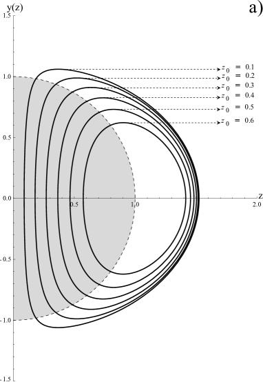
Figure 2: Magnetic dipole lines of a static charge in external magnetic field exampled with $B=\infty$. The pattern to be trusted inside the charge, $y^{2}+z^{2}<1$, following solution (83) with real $z_{0}$.

3.4.2 Exterior

Referring to the same basis and reference frame as in the previous Subsection, the magnetic field outside the sphere (67) reads

$$h_{i}^{\mathrm{out}}\left(\mathbf{x}\right) = B\left\{\left[\mathcal{A}^{\prime}+\left(\mathcal{B}^{\prime}+\mathcal{C}^{\prime}\right)y^{2}+\mathcal{D}^{\prime}y^{4}\right]e_{\left(3\right)i}+\left(\mathcal{C}^{\prime}+\mathcal{D}^{\prime}y^{2}\right)yze_{\left(1\right)i}\right\}$$

$$\mathcal{A}^{\prime} = \left(\frac{Ze}{4\pi r^{2}}\right)^{2}\left\{\frac{1}{2}\left(\mathcal{L}_{\mathfrak{FF}}-\mathcal{L}_{\mathfrak{GG}}-B^{2}\mathcal{L}_{\mathfrak{FGG}}\right)\right.$$

$$+ \left.\frac{r}{5R}\left(2\mathcal{L}_{\mathfrak{GG}}-3\mathcal{L}_{\mathfrak{FF}}+B^{2}\mathcal{L}_{\mathfrak{FGG}}\right)+\frac{9R}{35r}B^{2}\mathcal{L}_{\mathfrak{FGG}}\right\}$$

$$\mathcal{B}^{\prime} = \left(\frac{Ze}{4\pi r^{2}}\right)^{2}\frac{R^{2}}{r^{2}}\left(1-\frac{9R}{7r}\right)B^{2}\mathcal{L}_{\mathfrak{FGG}}\,,$$

$$\mathcal{D}^{\prime} = -3\left(\frac{Ze}{4\pi r^{2}}\right)^{2}\left(\frac{R}{r}\right)^{4}\left(1-\frac{R}{r}\right)B^{2}\mathcal{L}_{\mathfrak{FGG}}\,,$$

$$\mathcal{C}^{\prime} = \left(\frac{Ze}{4\pi r^{2}}\right)^{2}\left(\frac{R}{r}\right)^{2}\left\{2\left(-\mathcal{L}_{\mathfrak{FF}}+\frac{1}{2}\mathcal{L}_{\mathfrak{GG}}+B^{2}\mathcal{L}_{\mathfrak{FGG}}\right)\right.$$ (84)

$$+ \left.\frac{3r}{5R}\left(3\mathcal{L}_{\mathfrak{FF}}-2\mathcal{L}_{\mathfrak{GG}}-B^{2}\mathcal{L}_{\mathfrak{FGG}}\right)-\frac{9R}{7r}B^{2}\mathcal{L}_{\mathfrak{FGG}}\right\}$$

where $y=x_{3}/R$ and $z=x_{1}/R$. The ratio $h_{3}^{\mathrm{out}}\left(\mathbf{x}\right)/h_{1}^{\mathrm{out}}\left(\mathbf{x}\right)$ can be expressed as

$$\frac{h_{3}^{\mathrm{out}}\left(\mathbf{x}\right)}{h_{1}^{\mathrm{out}}\left(\mathbf{x}\right)} = \frac{\beta^{\prime}\left(y,z\right)}{yz}+\gamma^{\prime}\left(y,z\right)\frac{y}{z}+E^{\prime}\left(y,z\right)\frac{y^{3}}{z}\,,$$

$$\beta^{\prime}\left(y,z\right) = \frac{\mathcal{A}^{\prime}}{\mathcal{C}^{\prime}+\mathcal{D}^{\prime}y^{2}}\,,\ \ \gamma^{\prime}\left(y,z\right)=\frac{\mathcal{B}^{\prime}+\mathcal{C}^{\prime}}{\mathcal{C}^{\prime}+\mathcal{D}^{\prime}y^{2}}\,,\ \ E^{\prime}\left(y,z\right)=\frac{\mathcal{D}^{\prime}}{\mathcal{C}^{\prime}+\mathcal{D}^{\prime}y^{2}}\,,$$ (85)

Taking into account the asymptotic behavior at large magnetic field $B\gg m^{2}/e$ (81), the coefficients $\mathcal{A}^{\prime}$, $\mathcal{B}^{\prime}$, $\mathcal{D}^{\prime}$ and $\mathcal{C}^{\prime}$ are

$$\mathcal{A}^{\prime}=\left(\frac{Ze}{4\pi r^{2}}\right)^{2}\left(\frac{\alpha}{3\pi B}\right)\left(\frac{e}{m^{2}}\right)\left(\frac{x}{5R}\right)\left(1-\frac{9R^{2}}{7r^{2}}\right)\,,$$

$$\mathcal{B}^{\prime}=-\left(\frac{Ze}{4\pi r^{2}}\right)^{2}\left(\frac{\alpha}{3\pi B}\right)\left(\frac{e}{m^{2}}\right)\left(\frac{R^{2}}{r^{2}}\right)\left(1-\frac{9R}{7r}\right)\,,$$

$$\mathcal{D}^{\prime}=3\left(\frac{Ze}{4\pi r^{2}}\right)^{2}\left(\frac{\alpha}{3\pi B}\right)\left(\frac{e}{m^{2}}\right)\left(\frac{R}{r}\right)^{4}\left(1-\frac{R}{r}\right)\,,$$

$$\mathcal{C}^{\prime}=\left(\frac{Ze}{4\pi r^{2}}\right)^{2}\left(\frac{\alpha}{3\pi B}\right)\left(\frac{e}{m^{2}}\right)\left(\frac{R}{r}\right)^{2}\left(-1-\frac{3r}{5R}+\frac{9R}{7r}\right)\,,$$ (86)

then $\beta^{\prime}$, $\gamma^{\prime},$ and $E^{\prime}$ read

$$\beta^{\prime}\left(y,z\right)=-\frac{r^{3}}{5MR^{3}}\left(1-\frac{9R^{2}}{7r^{2}}\right)\,,$$

$$\gamma^{\prime}\left(y,z\right)=\frac{1}{M}\left(2+\frac{3r}{5R}-\frac{18R}{7r}\right)\,,$$

$$E^{\prime}\left(y,z\right)=-\frac{3R^{2}}{Mr^{2}}\left(1-\frac{R}{r}\right)\,,$$

$$M=1+\frac{3r}{5R}-\frac{9R}{7r}-3R^{2}\left(\frac{y}{r}\right)^{2}\left(1-\frac{R}{r}\right)\,.$$ (87)

Equating the derivative $dy/dz$ with the ratio $h_{3}^{\mathrm{out}}\left(\mathbf{x}\right)/h_{1}^{\mathrm{out}}\left(\mathbf{x}\right)$ (85) one finds the differential equation for the magnetic lines outside the sphere. Using (85)-(87) the differential equation has the final form

$$\frac{dy}{dz}=\frac{9R^{2}r^{4}-7r^{6}+\left(Rry\right)^{2}\left(21r^{2}+70Rr-90R^{2}\right)+105R^{5}y^{4}(R-r)}{R^{2}yz\left[r^{2}\left(21r^{2}+35Rr-45R^{2}\right)+105R^{3}y^{2}\left(R-r\right)\right]}\,.$$ (88)

This equation does not have analytic (closed) solutions. We found them by using numerical methods. The integration constant is fixed by the matching requirements with the pattern in Fig. 2: we demand that solutions of (79), for each fixed $z_{0}$, have the same numerical values as (88) at the border of the sphere $y^{2}+z^{2}=r^{2}/R^{2}=1$. In this way the continuous continuation of solutions of (79) to the outer region, where equation (88) is actual, is achieved. Figure 3-c) shows the overall pattern of magnetic lines to be trusted everywhere, wherefrom the lines beyond their domains of definition have been deleted. The values of $y\left(z\right)$ and $z$ at the border of the sphere are listed below for each integration constant $z_{0}$:

$$z_{0} = 0.1\rightarrow z\simeq 0.186\,,\ \ y\left(0.186\right)\simeq 0.983\,,$$

$$z_{0} = 0.2\rightarrow z\simeq 0.349\,,\ \ y\left(0.349\right)\simeq 0.973\,,$$

$$z_{0} = 0.3\rightarrow z\simeq 0.486\,,\ \ y\left(0.486\right)\simeq 0.874\,,$$

$$z_{0} = 0.4\rightarrow z\simeq 0.604\,,\ \ y\left(0.604\right)\simeq 0.797\,,$$

$$z_{0} = 0.5\rightarrow z\simeq 0.707\,,\ \ y\left(0.707\right)\simeq 0.707\,$$

$$z_{0} = 0.6\rightarrow z\simeq 0.8\,,\ \ y\left(0.8\right)\simeq 0.6\,.$$ (89)

The magnetic lines in 3-c) remind very much the standard pattern of those of a finite-thickness solenoid in classical magnetostatics.

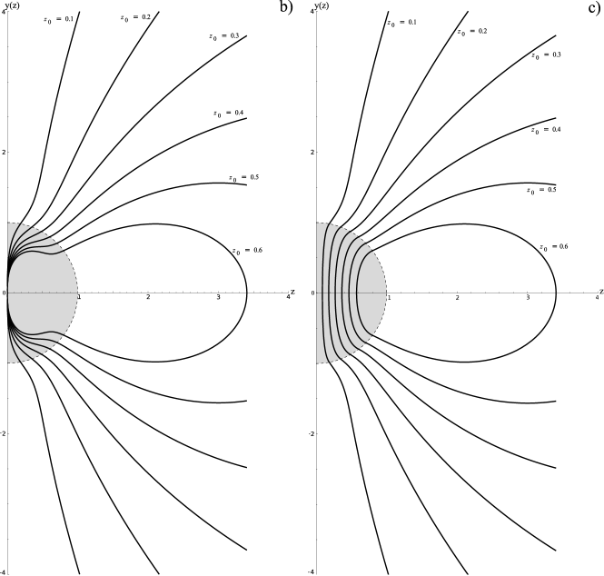
Figure 3: Magnetic dipole lines of a static charge in external magnetic field exampled with $B=\infty$. b) The pattern to be trusted outside the charge, $y^{2}+z^{2}>1$, following solution (88). For each choice of $z_{0}$ we extract from (83) the corresponding value for $y(z)$ at the border of the sphere. See (89) for some boundary conditions to (88). c) United pattern to be trusted throughout.

4 Beyond the spherical symmetry of the applied field

Here we search for an extension of (68) to spherically nonsymmetric applied electric field. Such generalization provides a more general form of the magnetic dipole moment $\boldsymbol{\mu}$.

Let us first see, how the result (68), (69) can be directly reproduced by considering long-range behavior of the magnetic response (37) to the spherically symmetric electric field (41), (42). According to (38) the field $\mathfrak{h}_{i}\left(\mathbf{x}\right)$ in the far-off domain reads

$$\mathfrak{h}_{i}\left(\mathbf{x}\right)\simeq\frac{1}{2r^{4}}\left(\frac{Ze}{4\pi}\right)^{2}\left[\left(\mathcal{L}_{\mathfrak{FF}}-\mathcal{L}_{\mathfrak{FGG}}\frac{\left(\mathbf{B\cdot x}\right)^{2}}{r^{2}}\right)B_{i}-2\mathcal{L}_{\mathfrak{GG}}\frac{\left(\mathbf{B\cdot x}\right)x_{i}}{r^{2}}\right]\,,$$ (90)

where we have restricted ourselves to the leading contribution at large $r=|\mathbf{x}|$. The leading behavior of the quantities $\mathfrak{I}_{k}\left(\mathbf{x}\right)$ in (37) is,

$$\mathfrak{I}_{k}(r)\simeq\frac{1}{r}\int d^{3}y\mathfrak{h}_{k}(\mathbf{y}),$$

provided that the integrals here converge. Then,

$$\partial_{i}\partial_{k}\mathfrak{I}_{k}(\mathbf{x})=\left(\frac{3x_{i}x_{k}}{r^{5}}-\frac{\delta_{ik}}{r^{3}}\right)\int d^{3}y\mathfrak{h}_{k}(\mathbf{y})\,.$$ (91)

The field $\mathfrak{h}_{i}\left(\mathbf{x}\right)$ (90) falls off faster than this, namely as $1/r^{4},$ hence its contribution into the first line of (37) can be neglected as compared to (91). So, the large-distance behavior of the nonlinear magnetic field $h_{i}\left(\mathbf{x}\right)$ (37) is just (91), i.e., that of a magnetic dipole. Its magnetic dipole moment $\mu_{i}^{\mathrm{LD}}$ is

$$\mu_{i}^{\mathrm{LD}}=\frac{1}{4\pi}\int d^{3}y\mathfrak{h}_{i}(\mathbf{y})\,,$$ (92)

$$\mathfrak{h}_{i}(\mathbf{y})=\frac{B_{i}}{2}\left(\mathcal{L}_{\mathfrak{FF}}\mathbf{E}^{2}\left(\mathbf{y}\right)-\mathcal{L}_{\mathfrak{FGG}}\left(\mathbf{B}\cdot\mathbf{E}\left(\mathbf{y}\right)\right)^{2}\right)-\mathcal{L}_{\mathfrak{GG}}\left(\mathbf{B}\cdot\mathbf{E}\left(\mathbf{y}\right)\right)E_{i}\left(\mathbf{y}\right)\,.$$

The result (92) agrees with the previous result (69) in case the spherically symmetric $\mathbf{E}$ is specialized to (39). To make sure of this it suffices to substitute expression (63) for $\mathfrak{h}_{i}(\mathbf{y})$ into (92) and fulfill the integration, which converges both at the lower, $y=0,$ and the upper, $y=\infty,$ limit.

However, the validity of the result (92) is much wider. For instance, let us take Eq. (33) or, equivalently, (34) for the scalar potential responsible for the remote cylindrically-symmetric electric field of a static extended charge $Q=Ze,$ whose density decreases sufficiently fast at infinity, but is otherwise arbitrary, not subject to any symmetry. Recall, that this cylindrical, instead of spherical, symmetry became in Sec. 2.1 the effect of the linear vacuum polarization in an external magnetic field. It is easy to make sure that when this electric field is substituted into (38) for $\mathfrak{h}_{i}\left(\mathbf{x}\right),$ the resulting expression in place of (90) also decreases as $1/r^{4},$ the same as it. Hence, we are left again with Eq. (91)  for the large-distance asymptote of the nonlinearly induced magnetic field $h_{i}\left(\mathbf{x}\right)$ (37). Since the electric field (34) is invariant under rotations around the external magnetic field $\mathbf{B,}$ the latter remains the only special direction in the space. Consequently, the magnetic moment (92) is directed along $\mathbf{B,}$ the same as (69).

5 Conclusion

In this work it was shown that a static charge, apart from being a source of the customary Coulomb-like electric field, is also a nonlinear source of a magnetic field. This field is generated due to a nonlinear induced current caused by a constant and homogeneous external magnetic field. As a result, the long-range magnetic field behaves like a magnetic field generated by a magnetic dipole moment. In other words, the extended charge has a long-range magnetic dipole character. The magnetic field lines resemble the well known magnetic dipole structure.

The validity of equations found here for the nonlinear magnetic response of the magnetic background to an applied electric field is restricted to the fields, smooth in time and space. They can be directly applied to charged large astrophysical objects, but lead to overestimation, where small objects as charged mesons and baryons are concerned. Therefore, to make such application reasonable, one needs to go beyond the infrared approximation. To this end QED calculations of three-photon diagram in an external magnetic field must be efficiently exploited beyond the photon mass shell. We hope to come back to this more complicated problem in future works.

Appendix

Performing derivations of the potential (39) leads to Dirac delta-functions and their derivatives as well. Taking into account smoothness conditions at $r=R$, one is able to simplify the explicit form of some quantities under consideration. One can see that,

$$a_{0}^{\mathrm{I}}\left(R\right)=a_{0}^{\mathrm{II}}\left(R\right)\,,\ \ \left.\frac{da_{0}^{\mathrm{I}}\left(r\right)}{dr}\right|_{r=R}=\left.\frac{da_{0}^{\mathrm{II}}\left(r\right)}{dr}\right|_{r=R}\,,\ \ \left.\frac{d^{2}a_{0}^{\mathrm{I}}\left(r\right)}{dr^{2}}\right|_{r=R}\neq\left.\frac{d^{2}a_{0}^{\mathrm{II}}\left(r\right)}{dr^{2}}\right|_{r=R}\,,$$ (93)

and higher derivatives are not continuous at $r=R$. In this way any function proportional to $da_{0}\left(r\right)/dr$,

$$\frac{da_{0}\left(r\right)}{dr}=\frac{da_{0}^{\mathrm{I}}\left(r\right)}{dr}\theta\left(R-r\right)+\frac{da_{0}^{\mathrm{II}}\left(r\right)}{dr}\theta\left(r-R\right)+\left(a_{0}^{\mathrm{II}}\left(r\right)-a_{0}^{\mathrm{I}}\left(r\right)\right)\delta\left(r-R\right)\,,$$ (94)

can be simplified  by omitting the Dirac delta-function terms. This simplification is supported by the fact that $\left(a_{0}^{\mathrm{II}}\left(r\right)-a_{0}^{\mathrm{I}}\left(r\right)\right)\delta\left(r-R\right)$ gives zero contribution, since

$$\int_{-\infty}^{\infty}drf\left(r\right)\left(a_{0}^{\mathrm{II}}\left(r\right)-a_{0}^{\mathrm{I}}\left(r\right)\right)\delta\left(r-R\right)=f\left(R\right)\left(a_{0}^{\mathrm{II}}\left(R\right)-a_{0}^{\mathrm{I}}\left(R\right)\right)=0\,,$$

where $f\left(r\right)$ represents any function, well-behaved at $r=R$. The same idea can be generalized to any function which depends on $d^{2}a_{0}\left(r\right)/dr^{2}$ or higher derivatives.

In order to evaluate the integrals $\mathfrak{I}_{k}\left(\mathbf{x}\right)$, which make part of the total magnetic field (37), one has to evaluate $v\left(r\right),\ u\left(r\right)$ and $w\left(r\right)$ (51)-(54). All of these functions can be conveniently written as sums of two other integrals. For example, we write (51) as $v\left(r\right)=\left(2\pi/r\right)\left[v_{1}\left(r\right)+v_{2}\left(r\right)\right]$ where,

$$v_{1}\left(r\right)=\int_{0}^{R}dy\left[\left(r+y-\left|r-y\right|\right)\frac{y^{3}}{R^{6}}\right]\,,\ \ v_{2}\left(r\right)=\int_{R}^{\infty}dy\left(\frac{r+y-\left|r-y\right|}{y^{3}}\right)\,.$$

Now, $v_{1}\left(r\right)$ can be calculated considering two situations, namely $r<R$ and $r>R$. Then

$$v_{1}\left(r\right) = \frac{1}{R^{6}}\left[\int_{0}^{r}dyy^{3}\left(2y\right)+\int_{r}^{R}dyy^{3}\left(2r\right)\right]=\frac{r}{2R}\left(1-\frac{r^{4}}{5R^{4}}\right)\,,\ \ r<R\,,$$

$$v_{1}\left(r\right) = \frac{2}{R^{6}}\int_{0}^{R}dyy^{4}=\frac{2}{5R}\,,\ \ r>R\,,$$

hence,

$$v_{1}\left(r\right)=\frac{r}{2R}\left(1-\frac{r^{4}}{5R^{4}}\right)\theta\left(R-r\right)+\frac{2}{5R}\theta\left(r-R\right)\,.$$ (95)

Similarly

$$v_{2}\left(r\right)=\frac{r}{R^{2}}\theta\left(R-r\right)+\left(\frac{2}{R}-\frac{1}{r}\right)\theta\left(r-R\right)\,.$$ (96)

Then (51) takes the final form (55).

Besides, it should be noted that $u\left(r\right)$ and $w\left(r\right)$ can be written in a simplified form,

$$x^{2}u\left(r\right) = \frac{1}{2}\left(\frac{3c\left(r\right)}{r^{2}}-v\left(r\right)\right)\,,\ \ w(r)=\frac{1}{2}\left(v\left(r\right)-\frac{c\left(r\right)}{r^{2}}\right)\,,$$

$$c\left(r\right) = 2\pi r^{2}\int_{0}^{\infty}dyy^{4}\mathcal{E}^{2}\left(y\right)V_{2}\left(r,y\right)\,,$$ (97)

such that after finding $c\left(r\right)$ we can immediately derive $u\left(r\right)$ and $w\left(r\right)$. Thus, using the angular integral (50), the function $c\left(r\right)$ takes the form

$$c\left(r\right)=\frac{4\pi}{15r}\left[\int_{0}^{r}dy\left(5r^{2}y^{4}+2y^{6}\right)\mathcal{E}^{2}\left(y\right)+\int_{r}^{\infty}dy\left(2r^{5}y+5r^{3}y^{3}\right)\mathcal{E}^{2}\left(y\right)\right]\,.$$ (98)

Considering again $r<R$ and $r>R$, separately, we list below each integral appearing above:

$$\int_{0}^{r}dy\left(5r^{2}y^{4}+2y^{6}\right)\frac{\theta\left(R-y\right)}{R^{6}}=\frac{9r^{7}}{7R^{6}}\theta\left(R-r\right)+\left(\frac{7r^{2}+2R^{2}}{7R}\right)\theta\left(r-R\right)\,;$$

$$\int_{0}^{r}dy\left(5r^{2}y^{4}+2y^{6}\right)\frac{\theta\left(y-R\right)}{y^{6}}=\left(\frac{5r^{2}-3rR-2R^{2}}{R}\right)\theta\left(r-R\right)\,;$$

$$\int_{r}^{\infty}dy\left(2r^{5}y+5r^{3}y^{3}\right)\frac{\theta\left(R-y\right)}{R^{6}}=\left(\frac{5r^{3}}{4R^{2}}+\frac{r^{5}}{R^{4}}-\frac{9r^{7}}{4R^{6}}\right)\theta\left(R-r\right)\,;$$

$$\int_{r}^{\infty}dy\left(2r^{5}y+5r^{3}y^{3}\right)\frac{\theta\left(y-R\right)}{y^{6}}=\frac{r^{3}}{R^{2}}\left(\frac{r^{2}}{2R^{2}}+\frac{5}{2}\right)\theta\left(R-r\right)+3r\theta\left(r-R\right)\,.$$

Substituting these results in (98) and using (97), the scalar functions take their final form (56).

References

- [1] D. M. Gitman and A. E. Shabad, Phys. Rev. D 86, 125028 (2012); arXiv:1209.6287.
- [2] C. V. Costa, D.M. Gitman, and A.E.Shabad, Phys. Rev. D 88, 085026 (2013), arXiv:1307.1802 [hep-th] (2013).
- [3] G. Mie, Ann. der Phys. 342, 511 (1912).
- [4] T. Erber, Rev. Mod Phys. 38, 626 (1966).
- [5] Z. Bialynicka-Birula and I. Bialynicki-Birula, Phys. Rev. D 2, 2341 (1970).
- [6] W. Dittrich and H. Gies, Springer Tracts Mod. Phys. 166, 1 (2000).
- [7] F. Karbstein, arXiv:1308:6184.
- [8] A. E. Shabad and V. V. Usov, Phys. Rev. D 81, 125008 (2010).
- [9] H. Gies, F.Karbstein, and N. Seegert, New Journ. Phys. 15, 083002 (2013), arXiv:1305:2320[hep-ph].
- [10] S. P. Gavrilov and D. M. Gitman, Phys. Rev. D 87, 125025 (2013), arXiv:1211.6776.
- [11] A. Di Piazza, C. Muller, K.Z. Hatsagortsyan, and C.H. Keitel, Rev. Mod. Phys. 84, 1177 (2012), arXiv:1111:3886 [hep-ph].
- [12] A. E. Shabad and V. V. Usov, Nature 295, 215 (1982).
- [13] A. E. Shabad and V. V. Usov, Astrophys. Space Sci 117, 309 (1985); 128, 377 (1986); V. V. Usov and A. E. Shabad, Pis’ma Zh. Eksp. Teor. Fiz. 42, 17 (1985) (Sov. Phys. JETP Lett. 42, 19 (1985)).
- [14] A.E. Shabad and V.V. Usov, Phys. Rev. Lett. 98, 180403 (2007); arXiv: 0707.3475; A.E. Shabad and V.V. Usov, Phys. Rev. D 77, 025001 (2008);“String-Like Electrostatic Interaction from QED with Infinite Magnetic Field.” in: “Particle Physics on the Eve of LHC” (Proc. of the 13th Lomonosov Conference on Elementary Particle Physics, Moscow, August 2007), Ed. A.I. Studenikin, World Scientific, Singapore, 392 (2009), arXiv:0801.0115 [hep-th].
- [15] N. Sadooghi and A. Sodeiri Jalili, Phys. Rev. D 76, 065013 (2007).
- [16] B. Machet and M. I. Vysotsky, Phys. Rev. D 83, 025022 (2011).0115 [hep-th].
- [17] V.N. Oraevskii, A.I. Rez, and V.B. Semikoz, Zh. Eksp. Teor. Fiz. 72, 820 (1977) [Sov. Phys. JETP 45, 428 (1977)], S. I. Godunov, B. Machet and M. I. Vysotsky, Phys. Rev. D 85, 044058 (2012).
- [18] A.E. Shabad and V.V. Usov, Phys. Rev .Lett. 96, 180401 (2006), Phys. Rev. D 73, 125021 (2006).
- [19] S.L. Adler, J.N. Bahcall, C.G. Callan, and M.N. Rosenbluth, Phys. Rev. Lett. 25, 1061 (1970); S.L. Adler, Ann. Phys. (N.Y.) 67, 599 (1971).
- [20] R.J. Stoneham, J.Phys. A: Math. Gen., 12, 2187 (1979).
- [21] S.L. Adler and C. Schubert, Phys. Rev. Lett. 77, 1695 (1996); M. Mentzel, D. Berg, G. Wunner, Phys. Rev. D 50, 1125 (1994); M.V. Chistyakov, A.V. Kuznetsov, and N.V. Mikheev, Phys. Lett. B 434, 67 (1998), Yad. Fiz. 62, 1638 (1999); M.G. Baring, Phys. Rev. D 62, 016003 (2000); J.I. Weise, M.G. Baring, and D.B. Melrose, Phys. Rev. D 57, 5526 (1998); C. Wilke and G. Wunner, Phys. Rev. D 55,997 (1997); V. N. Baier, A. I. Mil’shtein, and R. Zh. Shaisultanov, Phys. Rev. Lett. 77, 1691 (1996), Zh. Eksp. Teor. Fiz. 111, 52 (1997) [Sov. Phys. JETP 84, 29 (1997)].
- [22] V.O. Papanyan and V.I. Ritus, Sov. Phys. JETP 34, 1195 (1972); 38, 879 (1974).
- [23] V. B. Berestetsky, E. M. Lifshits, and L. P. Pitayevsky, Quantum Electrodynamics (Nauka, Moscow, 1989; Pergamon Press, Oxford, New York, 1982).
- [24] S. Weinberg, The Quantum Theory of Fields, (University Press, Cambridge, 2001).
- [25] E.H.Wichmann and N. M. Kroll, Phys. Rev. 96, 232 (1954); 101, 843 (1956).
- [26] T. C. Adorno, D. M. Gitman, A. E. Shabad and D. V. Vassilevich, Phys. Rev. D 84, 085031 (2011); 84, 065003 (2011); T. C. Adorno, D. M. Gitman and A. E. Shabad, Phys. Rev. D 86, 027702 (2012).
- [27] I. A. Batalin and A.E. Shabad, Zh. Eksp. Teor .Fiz. 60, 894 (1971) [ Sov. Phys . JETP 33, 483 (1971)], A. E. Shabad, Lett. Nuovo Cimento 3, 457 (1972); A. E. Shabad, Ann. Phys. 90, 166 (1975), A. E. Shabad, Polarization of the Vacuum and Quantum Relativistic Gas in an External Field (Nova Science Publishers, New York 1991). See also in Polarization effects in an external gauge fields Ed. V. L. Ginzburg, Proc. P. N. Lebedev Phys. Inst. 192,05 (Nauka, Moscow, 1988) in Russian.
- [28] V.I. Ritus, in Issues in Intense-Field Quantum Electrodynamics, Proc. Lebedev Phys. Inst. 168, 5, Ed. V. L. Ginzburg (Nauka, Moscow, 1986; Nova Science Publ., New York , 1987).
- [29] M. Born and L. Infeld, Proc. Roy. Soc. A 144, 425 (1934).
- [30] A.E. Shabad and V.V. Usov, Phys. Rev. D 83, 105006 (2011).
- [31] S. V.-Chavez and A.E. Shabad, Phys. Rev. D 86, 105040 (2012).
- [32] T. C. Adorno, D. M. Gitman, A. E. Shabad, “Electric charge is a magnetic dipole when placed in a background magnetic field ”, arXiv:1402.3848 [hep-th] (2014), Phys. Rev. D 89, 047504 (2014)
- [33] I. S. Gradshtein, N. M. Ryzhik, Tables of Integrals, Series and Products, 70th Ed., Academic Press, 2007.
- [34] E. Kamke, Differentialgleihungen. Lösungsmethoden und Lösungen: I.Gewöhnliche Differentialgleihungen (Part II) (Leipzig: Akademische Verlagsgesellschaft, 1959).
- [35] W. Heisenberg and H. Euler, Z. Phys. 98, 714 (1936); V. Weiskopf, K. Dan. Vidensk. Selsk. Mat. Fys. Medd. 14, 6 (1936); J. Schwinger, Phys. Rev. 82, 664 (1951); V.B. Berestetsky, E.M. Lifshits, and L.P. Pitayevsky.