Polynomial-time Solvable #CSP Problems
via Algebraic Models and Pfaffian Circuits

Abstract

A Pfaffian circuit is a tensor contraction network where the edges are labeled with changes of bases in such a way that a very specific set of combinatorial properties are satisfied. By modeling the permissible changes of bases as systems of polynomial equations, and then solving via computation, we are able to identify classes of 0/1 planar #CSP problems solvable in polynomial-time via the Pfaffian circuit evaluation theorem (a variant of L. Valiant’s Holant Theorem). We present two different models of 0/1 variables, one that is possible under a homogeneous change of basis, and one that is possible under a heterogeneous change of basis only. We enumerate a series of 1,2,3, and 4-arity gates/cogates that represent constraints, and define a class of constraints that is possible under the assumption of a “bridge” between two particular changes of bases. We discuss the issue of planarity of Pfaffian circuits, and demonstrate possible directions in algebraic computation for designing a Pfaffian tensor contraction network fragment that can simulate a swap gate/cogate. We conclude by developing the notion of a decomposable gate/cogate, and discuss the computational benefits of this definition.

1 Introduction

A solution to a constraint satisfaction problem (CSP) is an assignment of values to a set of variables such that certain constraints on the combinations of values are satisfied. A solution to a counting constraint satisfaction problem (#CSP) is the number of solutions to a given CSP. For example, the classic NP-complete problem 3-SAT is a CSP problem, but counting the number of satisfying assignments is a #CSP problem. CSP and #CSP problems are ubiquitous in computer science, optimization and mathematics: they can model problems in fields as diverse as Boolean logic, graph theory, database query evaluation, type inference, scheduling and artificial intelligence. This paper uses computational commutative algebra to study the classification of #CSP problems solvable in polynomial-time by Pfaffian circuits.

In a seminal paper [valiant_ha], Valiant used “matchgates” to demonstrate polynomial-time algorithms for a number of #CSP problems, where none had been previously known before. Pfaffian circuits [lands_hol_wo_mg, morton_pfaff, morton2013generalized] are a simplified and extensible reformulation of Valiant’s notion of a holographic algorithm, which builds on J.Y. Cai and V. Choudhary’s work in expressing holographic algorithms in terms of tensor contraction networks [cai_mg_ten]. Valiant’s Holant Theorem ([valiant_qc, valiant_ha]) is an equation where the left-hand side has both an exponential number of terms and an exponential number of term cancellations, whereas the right-hand side is computable in polynomial-time. Extensions to holographic algorithms made possible by Pfaffian circuits include swapping out this equation for another combinatorial identity [morton2013generalized], viewing this equation as an equivalence of monoidal categories [morton2013generalized], or, as is done here, using heterogeneous changes of bases with the aid of computational commutative algebra.

In a series of papers ([bulatov_dalmau_maltsev, bulatov_dalmau_towdic, bulatov_grohe]) culminating in [bulatov_dic, bulatov2013complexity], A. Bulatov explored the problem of counting the number of homomorphisms between two finite relational structures (an equivalent statement of the general #CSP problem). In [bulatov_dic, bulatov2013complexity], Bulatov demonstrates a complete dichotomy theorem for #CSP problems. In other words, Bulatov demonstrates that a #CSP problem is either in FP (solvable in polynomial time), or it is #P-complete. However, not only does his paper rely on an thorough knowledge of universal algebras, but it relies on the notion of a congruence singular finite relational structure, and the complexity of determining if a given structure has this property is unknown (perhaps even undecidable). However, in 2010, Dyer and Richerby [dyer2010effective] offered a simplified proof of Bulatov’s result, and furthermore established a new criterion (known as strong balance) for the #CSP dichotomy that is not only decidable, but is in fact in NP.

In light of these elegant and conclusive dichotomy theorems, research on #CSP problems focused in a different direction. The dichotomy theorems were specialized to categorize both 0/1 and finite alphabets [bulatov_fa, cai2012complexity], and also specialized for restricted input cases such as planar instances, symmetric signatures, or homogeneous change of basis [cai_lu_xia:dichotomy]. This paper begins the process of developing a dichotomy theorem for Pfaffian circuits under a non-homogeneous (heterogeneous) change of basis by identifying classes of symmetric and asymmetric planar 0/1 polynomial-time solvable instances via algebraic methods and computation. It is the first systematic exploration of the heterogeneous basis case.

For clarity, we list four main reasons for this approach. First, since the time complexity of determining the Pfaffian of a matrix is equivalent to that of finding the determinant, our approach is not only polynomial-time, but $O(n^{\omega_{p}})$ (where $1.19\leq\omega_{p}\leq 3$ and $n$ is the total number of variable inclusions in the clauses). We observe that Valiant’s matchgate approach has a similar time complexity; however, the tensor contraction network representation of the underlying #CSP instance is often a more compact representation than that of the matchgate encoding. Second, our approach is based on algebraic computational methods, and thus, any independent innovations to Gröbner basis algorithms (or determinant algorithms, for that matter) will make it easier to classify problems. Third, by approaching Pfaffian circuits via algebraic computation, we are able to consider non-homogeneous (heterogeneous) changes of bases, an option which has not yet been explored. The use of a heterogeneous changes of bases brings us to our final reason for considering Pfaffian circuits: the gates/cogates may be decomposable into smaller gates/cogates in such a way that lower degree polynomials are used, which exponentially enhances the performance of this method.

We begin Sec. 2 with a detailed introduction to tensor contraction networks, which can be skipped by those already familiar with these ideas. We next recall the definition of Pfaffian gates/cogates, and their connection to classical logic gates (OR, NAND, etc.). In Sec. 2.5, we define Pfaffian circuits, and give a step-by-step example of evaluating a Pfaffian circuit via the polynomial-time Pfaffian circuit evaluation theorem [morton_pfaff]. In Sec. 3, we present the new algebraic and computational aspect of this project: given a gate/cogate, we describe a system of polynomial equations such that the solutions (if any) are in bijection to the changes of bases (not necessarily homogeneous) where the gate/cogate is “Pfaffian”. By “linking” the ideals associated with these gates/cogates together, and then solving using software such as Singular [singular], we begin the process of characterizing the building blocks of Pfaffian circuits.

In Sec. 4, we present the first results of our computational exploration. We demonstrate two different ways of simulating 0/1 variables as planar, Pfaffian, tensor contraction network fragments. The first uses a homogeneous change of a basis, and the second (known as a Boolean tree) is possible under a heterogeneous change of basis only. We use the Boolean trees to develop two classes of compatible constraints, the first of which identifies gates/cogates that are Pfaffian under a homogeneous change of basis, and the second of which utilizes the two existing changes of bases ($A$ and $B$), and then posits the existence of a third change of basis $C$, to identify 24 additional Pfaffian gates/cogates. Thus, Sec. 4 begins the process of characterizing (via algebraic computation) planar, Pfaffian, 0/1 #CSP problems that are solvable in polynomial-time.

In Sec. 5, we investigate the question of planarity. Within the Pfaffian circuit framework, the addition of a swap gate/cogate is not equivalent to lifting the planarity restriction, since the compatible gates/cogates representing solvable #CSP problems are not automatically identifiable. Thus, there are no inherent complexity-theoretic stumbling blocks to investigating a Pfaffian swap gate/cogate, and indeed the hope is that such an investigation would eventually yield a new sub-class of non-planar poloynomial-time solvable #CSP problems. However, in this paper, we only demonstrate that specific gates which can be used as building blocks for a swap gate (such as CNOT) are indeed Pfaffian (under a heterogeneous change of basis only). We then describe several attempts to construct a Pfaffian swap gate, indicating precisely where the attempts fail, and conclude by presenting a partial swap gate. This result suggests a specific direction (in both algebraic computation and combinatorial structure), for constructing a Pfaffian swap gate. We conclude in Sec. 6 by introducing the notion of a decomposable gate/cogate, and discussing the computational advantages of gate decompositions.

To summarize, this project models Pfaffian circuits as systems of polynomial equations, and then solves the systems using Singular [singular], with the goal of identifying classes of planar 0/1 #CSP problems that are solvable in polynomial-time.

2 Background and Definitions of Pfaffian Circuits

In this section, we develop the necessary background for modeling #CSP problems as Pfaffian circuits, and then solving them via the Pfaffian circuit evaluation theorem [morton_pfaff]. We begin with tensors and the convenience of the Dirac (bra/ket) notation from quantum mechanics, and then express Boolean predicates (which we call gates/cogates) as elements of a tensor product space. We then describe the process of applying a change of basis to these gates/cogates such that they are expressible as tensors with coefficients that are the sub-Pfaffians of some skew-symmetric matrix. We conclude with a step-by-step example of solving a particular Pfaffian circuit with the Pfaffian circuit evaluation theorem.

2.1 Tensors and Dirac Notation

Let $U$ and $V$ be two-dimensional complex vector spaces equipped with bases, with $v\in V$ and $u\in U$. In the induced basis we can express the tensor product $v\otimes u$ as the Kronecker product, the vector $w\in\mathbb{C}^{4}$ ($w=[w_{0},w_{1},w_{2},w_{3}]^{T}$) with $w_{2i+j}=v_{i}u_{j}$ for $0\leq i,j\leq 1$. For example,

$$\left[\begin{array}[]{c}3\\ 1/3+i\end{array}\right]\otimes\left[\begin{array}[]{c}1+2i\\ 1/2\end{array}\right]=\left[\begin{array}[]{c}\hskip 13.0pt3\hskip 15.0pt\left[\begin{array}[]{c}1+2i\\ 1/2\end{array}\right]\\ (1/3+i)\left[\begin{array}[]{c}1+2i\\ 1/2\end{array}\right]\\ \end{array}\right]=\left[\begin{array}[]{c}3+6i\\ 3/2\\ -5/3+5/3i\\ 1/6+i/2\end{array}\right]~{}.$$

Now let $V_{1},\ldots,V_{n}$ each be isomorphic to $\mathbb{C}^{2}$, and let $\{v^{0}_{i},v^{1}_{i}\}$ be a basis of $V_{i}$. Any induced basis vector in the tensor product space $V_{1}\otimes V_{2}\otimes\cdots\otimes V_{n}$ can be concisely written as a ket, where $v^{0}$ is denoted by $|0\rangle$ and $v^{1}$ is denoted by $|1\rangle$. For example, a basis element of $V_{1}\otimes V_{2}\otimes\cdots\otimes V_{n}$ can be written as

$$\underbrace{|1101\cdots 01\rangle}_{\text{ket}}~{} =v^{\mathbf{1}}_{1}\otimes v^{\mathbf{1}}_{2}\otimes v^{\mathbf{0}}_{3}\otimes v^{\mathbf{1}}_{4}\otimes\cdots\otimes v^{\mathbf{0}}_{n-1}\otimes v^{\mathbf{1}}_{n}~{},$$

and an arbitrary vector $w\in V_{1}\otimes V_{2}\otimes\cdots\otimes V_{n}$ can be written as

$$w =\alpha_{1}\underbrace{|00\cdots 0\rangle}_{\text{ket}}+\alpha_{2}\underbrace{|10\cdots 0\rangle}_{\text{ket}}+\cdots+\alpha_{2^{n}}\underbrace{|11\cdots 1\rangle}_{\text{ket}}~{},\quad\text{with~{}}\alpha_{1},\cdots,\alpha_{2^{n}}\in\mathbb{C}~{}.$$

Given a vector space $V$, the dual vector space $V^{*}$ is the vector space of all linear functions on $V$. Given $V_{1},\ldots,V_{n}$, let $V^{*}_{1},\ldots,V^{*}_{n}$ be their duals, with $\{\nu^{0*}_{i},\nu^{1*}_{i}\}$ the dual basis of $V^{*}_{i}$. We write a linear function in the tensor product space $V^{*}_{1}\otimes\cdots\otimes V^{*}_{n}$ as a bra, with $\nu^{0*}$ denoted by $\langle 0|$ and $\nu^{1*}$ denoted by $\langle 1|$. For example, a basis element can be written as

$$\underbrace{\langle 1101\cdots 01|}_{\text{bra}} =\nu^{\mathbf{1}*}_{1}\otimes\nu^{\mathbf{1}*}_{2}\otimes\nu^{\mathbf{0}*}_{3}\otimes\nu^{\mathbf{1}*}_{4}\otimes\cdots\otimes\nu^{\mathbf{0}*}_{n-1}\otimes\nu^{\mathbf{1}*}_{n}~{},$$

and an arbitrary linear function $w\in V^{*}_{1}\otimes V^{*}_{2}\otimes\cdots\otimes V^{*}_{n}$ can be written as

$$w =\beta_{1}\underbrace{\langle 00\cdots 0|}_{\text{bra}}+\beta_{2}\underbrace{\langle 10\cdots 0|}_{\text{bra}}+\cdots+\beta_{2^{n}}\underbrace{\langle 11\cdots 1|}_{\text{bra}}~{},\quad\text{with~{}}\beta_{1},\cdots,\beta_{2^{n}}\in\mathbb{C}~{}.$$

We may use subscripts to identify sub-tensor-products: for example, $|0_{6}1_{9}0_{11}\rangle$ denotes the induced basis element $v^{0}_{6}\otimes v^{1}_{9}\otimes v^{0}_{11}$ in the tensor product space $V_{6}\otimes V_{9}\otimes V_{11}$ (and similarly for the bras).

The dual basis element $\nu^{j*}_{i}$ with $j\in\{0,1\}$ yields a Kronecker delta function:

$$\nu^{j*}_{i}(v^{k}_{i})=\begin{cases}1&\text{if $j=k$~{},}\\ 0&\text{otherwise~{}.}\end{cases}$$

In the bra-ket notation, this is expressed as a contraction; e.g.  $\langle 0|0\rangle=1$ and $\langle 0|1\rangle=0$.

In classical computing, a bit takes on the value of 0 or 1. In quantum computing, given an orthonormal basis $\big{\{}|0\rangle,|1\rangle\big{\}}$, a pure state of a qubit is given by the superposition of states, denoted $\alpha|0\rangle+\beta|1\rangle$, with $\alpha^{2}+\beta^{2}=1$ and $\alpha,\beta\in\mathbb{C}$.

2.2 Boolean Predicates as Tensor Products

A Boolean predicate is a 0/1-valued function where the true/false output is dependent on the true/false input assignments of the variables. Here we see the 2-input Boolean predicate OR represented as both a bra and a ket.

OR = 0 0 0 1 0 1 0 1 1 1 1 1

OR (as a ket) $$=0\cdot|00\rangle+1\cdot|10\rangle+1\cdot|01\rangle+1\cdot|11\rangle~{}$$

$$=|10\rangle+|01\rangle+|11\rangle~{},\quad\text{and}$$

OR (as a bra) $$=\langle 10|+\langle 01|+\langle 11|~{}.$$

A Boolean predicate represented as a ket is a gate, and a Boolean predicate represented as a bra is a cogate. Just as Boolean predicates can be connected to describe a (counting) constraint satisfaction problems, these gates and cogates can be connected to describe a tensor contraction network.

2.3 Tensor Contraction Networks

A bipartite graph $G=\{X,Y,E\}$ is a graph partitioned into two disjoint vertex sets, $X$ and $Y$, such that every edge in the graph is incident on a vertex in both $X$ and $Y$. A bipartite tensor contraction network $\Gamma$ is a bipartite graph partitioned into gates and cogates. If $\Gamma$ contains $m$ edges, we consider the vector spaces $V_{1},\ldots,V_{m}$ (and vector space duals $V^{*}_{1},\ldots,V^{*}_{m}$) , and every vertex in $\Gamma$ is labeled with either a gate or cogate. Consider a vertex of degree $d$ which is incident on edges $e_{1},\ldots,e_{d}$. Then, the gate (or cogate) associated with that vertex is an element of the tensor product space $V_{e_{1}}\otimes\cdots\otimes V_{e_{d}}$ (or $V^{*}_{e_{1}}\otimes\cdots\otimes V^{*}_{e_{d}}$, respectively). We denote the tensor contraction network $\Gamma$ as the 3-tuple $\{G,C,E\}$ consisting of gates, cogates and edges. Every tensor contraction network considered in this paper is bipartite.

Example 1.

Consider the following tensor contraction network $\Gamma$ with arbitrary gates/cogates:

$$\quad\Gamma =\begin{cases}G=\begin{cases}G_{1}=|0_{4}0_{5}0_{6}\rangle+|1_{4}1_{5}1_{6}\rangle~{},\\ G_{2}=|1_{1}0_{2}1_{3}\rangle+|0_{1}1_{2}1_{3}\rangle+|1_{1}1_{2}1_{3}\rangle~{},\end{cases}\\ C=\begin{cases}C_{1}=\langle 0_{3}1_{6}|+\langle 1_{3}0_{6}|~{},\\ C_{2}=\langle 0_{2}1_{5}|+\langle 1_{2}0_{5}|~{},\\ C_{3}=\langle 1_{1}1_{4}|~{},\end{cases}\\ E=\{1,\ldots,6\}~{}.\end{cases}$$

Gates are denoted by boxes ($\Box$) and cogates by circles ($\circ$). Note that gate $G_{2}$ is incident on edges $1,2$ and $3$, and is an element of the tensor product space $V_{1}\otimes V_{2}\otimes V_{3}$. Similarly, cogate $C_{3}$ is incident on edges $1$ and $4$, and $C_{3}\in V^{*}_{1}\otimes V^{*}_{4}$. $\Box$

Given a tensor contraction network $\Gamma$, the value of the tensor contraction network, denoted $val(\Gamma)$, is the contraction of all the tensors in $\Gamma$. The value of any bipartite tensor contraction network is a scalar. We observe that the value of the tensor contraction network $\Gamma$ in Ex. 1 is $0$ (see Sec 2.5 for a contraction example).

2.4 Pfaffian Gates, Cogates and Circuits

In the previous section, we defined gates/cogates as the fundamental building blocks of tensor contraction networks. In this section, we describe how to find the value of a tensor contraction network in polynomial-time when the network satisfies certain combinatorial and algebraic conditions. In particular, we describe what it means for an individual gate/cogate to be Pfaffian.

An $n\times n$ skew-symmetric matrix $A$ has $a_{ij}=-a_{ji}$, and thus $a_{ii}=0$. For $n$ odd, the determinant of a skew-symmetrix matrix $A$ is zero, and for $n$ even, $\det(A)$ can be written as the square of a polynomial known as the Pfaffian of $A$. Given an even integer $n$, let $S^{\text{Pf}}_{n}\subseteq S_{n}$ be the set of permutations $\sigma\in S_{n}$ such that $\sigma(1)<\sigma(2),\sigma(3)<\sigma(4),\ldots,\sigma({n-1})<\sigma(n)$, and $\sigma(1)<\sigma(3)<\sigma(5)<\cdots<\sigma({n-1})$. Then, the Pfaffian of an $n\times n$ skew-symmetric matrix $A$, denoted $\text{Pf}(A)$, is given by

$$\text{Pf}(A)=\begin{cases}0~{},&\text{for $n$ odd}~{},\\ 1~{},&\text{for $n=0$}~{},\end{cases}~{},\quad\text{and}\quad\text{Pf}(A)=\overbrace{\sum\limits_{\sigma\in S^{\text{Pf}}_{n}}\text{sgn}(\sigma)a_{\sigma(1),\sigma(2)}a_{\sigma(3),\sigma(4)}\cdots a_{\sigma({n-1}),\sigma(n)}}^{\text{for $n$ even}}~{},$$

and $\big{(}\text{Pf}(A)\big{)}^{2}=\det(A)$. For example, if $A$ is a $2\times 2$ matrix, then $\text{Pf}(A)=a_{12}$. If $A$ is a $4\times 4$ matrix, then $\text{Pf}(A)=a_{12}a_{34}-a_{13}a_{24}+a_{14}a_{23}$. Laplace expansion can also be used to compute $\text{Pf}(A)$. For example, if $A$ is a $6\times 6$ matrix, then $\text{Pf}(A)=a_{12}\text{Pf}(A|_{3456})-a_{13}\text{Pf}(A|_{2456})+a_{14}\text{Pf}(A|_{2356})-a_{15}\text{Pf}(A|_{2346})+a_{16}\text{Pf}(A|_{2345})$, where $A|_{2356}$ is the submatrix of $A$ consisting only of the rows and columns indexed by $\{2,3,5,6\}$.

Let $[n]=\{1,\ldots,n\}$, and $I\subseteq[n]$. Then $|I\rangle$ is the ket corresponding to subset $I$. For example, given $I=\{2,5,7\}\subseteq[8]$, then $|I\rangle=|01001010\rangle$. Additionally, given $J=\{1,2,4,6,8\}\subseteq[8]$, then $J^{C}$ is the set of integers not present in $J$, or $J^{C}=\{3,5,7\}$.

Definition 1.

[morton_pfaff, lands_hol_wo_mg] Given an $n\times n$ skew-symmetric matrix $\Xi$, we define the subPfaffian of $\Xi$ and the subPfaffian dual of $\Xi$, denoted by $\text{\emph{sPf}}(\Xi)$ and $\text{\emph{sPf}}^{*}(\Xi)$ respectively, as

$$\text{\emph{sPf}}(\Xi) =\sum_{I\subseteq[n]}\text{\emph{Pf}}(\Xi|_{I})|I\rangle~{},\quad\quad\text{\emph{sPf}}^{*}(\Xi)=\sum_{J\subseteq[n]}\text{\emph{Pf}}(\Xi|_{J^{C}})\langle J|~{},$$

where $\Xi|_{I}$ is the submatrix of $\Xi$ with rows/columns indexed by $I$ (and similarly for $\Xi|_{J^{C}}$).

Example 2.

Given the $4\times 4$ skew-symmetric matrix $\Xi$, we calculate $\text{\emph{sPf}}(\Xi),\text{\emph{sPf}}^{*}(\Xi)$:

$$\Xi=\left[\begin{array}[]{cccc}0&i&0&2\\ -i&0&-1&0\\ 0&1&0&3\\ -2&0&-3&0\end{array}\right],$$

$$\text{\emph{sPf}}(\Xi) =\text{\emph{Pf}}(\Xi|_{\emptyset})|0000\rangle+\text{\emph{Pf}}(\Xi|_{1})|1000\rangle+\cdots+\text{\emph{Pf}}(\Xi|_{1234})|1111\rangle~{}$$

$$=|0000\rangle+i|1100\rangle+2|1001\rangle-|0110\rangle+3|0011\rangle+(-2+3i)|1111\rangle~{},$$

$$\text{\emph{sPf}}^{*}(\Xi) =\text{\emph{Pf}}(\Xi|_{1234})\langle 0000|+\text{\emph{Pf}}(\Xi|_{234})\langle 1000|+\cdots+\text{\emph{Pf}}(\Xi|_{\emptyset})\langle 1111|~{}$$

$$=(-2+3i)\langle 0000|+3\langle 1100|-\langle 1001|+2\langle 0110|+i\langle 0011|+\langle 1111|~{}.$$

We observe that, while $\text{\emph{Pf}}(\Xi)=-2+3i$ is a scalar, $\text{\emph{sPf}}(\Xi)$ is an element of the tensor product space $V_{1}\otimes\cdots\otimes V_{4}$ and $\text{\emph{sPf}}^{*}(\Xi)$ is an element of $V^{*}_{1}\otimes\cdots\otimes V^{*}_{4}$. $\Box$

The value of a closed tensor network is invariant under the action of $\times_{i}\operatorname{GL}V_{i}$, with each $\operatorname{GL}V_{i}$ acting on the corresponding wire. To see this explicitly, we now apply a change of basis $A$ to an edge in a tensor contraction network.

Consider

$$\text{, where }A=\left[\begin{array}[]{cc}a_{00}&a_{01}\\ a_{10}&a_{11}\end{array}\right],\text{ and }A^{-1}=\frac{1}{\det(A)}\left[\begin{array}[]{cc}a_{11}&-a_{01}\\ -a_{10}&a_{00}\end{array}\right]~{}.$$

The choice of indexing the rows and columns from zero is a notational convenience which will become clear in Sec. 3. When the change of basis $A$ is applied to an edge, the contraction property $\langle 0|1\rangle=\langle 1|0\rangle=0$ and $\langle 0|0\rangle=\langle 1|1\rangle=1$ must be preserved, since applying a change of basis must not affect $val(\Gamma)$. Since every edge in a bipartite tensor contraction network is incident on both a gate and cogate, when we apply the change of basis to the gate, we find $A|0\rangle=a_{00}|0\rangle+a_{10}|1\rangle$, and $A|1\rangle=a_{01}|0\rangle+a_{11}|1\rangle$. When we apply the change of basis to the cogate, we find $A^{-1}\langle 0|=\det(A)^{-1}\big{(}a_{11}\langle 0|-a_{01}\langle 1|\big{)}$, and $A^{-1}\langle 1|=\det(A)^{-1}\big{(}-a_{10}\langle 0|+a_{00}\langle 1|\big{)}$. Note that

$$1=\langle 0|0\rangle =\Big{\langle}A^{-1}\langle 0|,~{}A|0\rangle\Big{\rangle}=\Big{\langle}\det(A)^{-1}\big{(}a_{11}\langle 0|-a_{01}\langle 1|\big{)},~{}a_{00}|0\rangle+a_{10}|1\rangle\Big{\rangle}~{}$$

$$=\frac{a_{11}a_{00}\langle 0|0\rangle+a_{11}a_{10}\langle 0|1\rangle-a_{01}a_{00}\langle 1|0\rangle-a_{01}a_{10}\langle 1|1\rangle~{}}{\det(A)}=\frac{a_{11}a_{00}-a_{01}a_{10}}{\det(A)}=1~{}.$$

Therefore, when the change of basis $A$ is applied to the gate, the change of basis $A^{-1}$ is applied to the cogate. For convenience, this is denoted as follows:

xx

is denoted as

We now present the notion of a Pfaffian gate/cogate. Recall that in a tensor contraction network, the number of edges incident on the gate/cogate is the arity of the gate/cogate. For example, in Ex. 1, cogate $C_{2}=\langle 0_{2}1_{5}|+\langle 1_{2}0_{5}|$ is incident on edges 2 and 5, and thus has arity two.

Definition 2.

An arity-$n$ gate $G$ is Pfaffian after a change of basis if there exists an $n\times n$ skew-symmetric matrix $\Xi$, an $\alpha\in\mathbb{C}$, and matrices $A_{1},\ldots,A_{n}\in\mathbb{C}^{2\times 2}$ such that

$$(A_{1}\otimes\cdots\otimes A_{n})G =\alpha\hskip 1.0pt\text{sPf}(\Xi)~{}.$$

An arity-$n$ cogate $C$ is Pfaffian after a change of basis if there exists an $n\times n$ skew-symmetric matrix $\Theta$, a $\beta\in\mathbb{C}$, and matrices $A_{1},\ldots,A_{n}\in\mathbb{C}^{2\times 2}$ such that

$$(A^{-1}_{1}\otimes\cdots\otimes A^{-1}_{n})C =\beta\hskip 1.0pt\text{sPf}^{*}(\Theta)~{}.$$

When $A_{1}=\cdots=A_{n}$, we say that $G$ is Pfaffian under a homogeneous change of basis. Otherwise, we say that $G$ is Pfaffian under a heterogeneous change of basis. When no change of basis is needed, we simply say that $G$ is Pfaffian (and similarly for cogates).

Example 3 (Pfaffian Gates and Cogates).

Consider the change of basis matrix $A$:

$$A=\left[\begin{array}[]{cc}\frac{1}{10}\big{(}-5^{3/4}+5^{5/4})&5^{-1/4}\\ \frac{1}{10}\big{(}-5^{3/4}-5^{5/4}\big{)}&5^{-1/4}\end{array}\right]~{}.$$

Consider the OR gate $|10\rangle+|01\rangle+|11\rangle$, and observe that

$$(A\otimes A)\big{(}|10\rangle+|01\rangle+|11\rangle\big{)} =|00\rangle-|11\rangle~{}=\alpha\hskip 2.0pt\text{\emph{sPf}}(\Xi)=\text{\emph{sPf}}\left(\left[\begin{array}[]{cc}0&-1\\[-6.45831pt] 1&0\end{array}\right]\right)~{}.$$

Additionally, consider the cogate $\langle 00|+\langle 11|$, and observe that

$$\big{(}A^{-1}\otimes A^{-1}\big{)}\big{(}\langle 00|+\langle 11|\big{)} =\beta\hskip 2.0pt\text{\emph{sPf}}^{*}(\Theta)~{}=\underbrace{\Big{(}\frac{\sqrt{5}}{2}-\frac{1}{2}\Big{)}}_{\beta}\text{\emph{sPf}}^{*}\left(\left[\begin{array}[]{cc}0&\frac{\sqrt{5}}{2}+\frac{3}{2}\\ -\big{(}\frac{\sqrt{5}}{2}+\frac{3}{2}\big{)}&0\end{array}\right]\right)~{}.$$

Therefore the gate $|10\rangle+|01\rangle+|11\rangle$ and the cogate $\langle 00|+\langle 11|$ are both Pfaffian under the homogeneous change of basis $A$. We observe that the change of basis matrix $A$ was found computationally via the algebraic method described in Sec. 3. $\Box$

A Pfaffian circuit [morton_pfaff] is a tensor contraction network where some change of basis (possibly the identity) has been applied to every edge such that every gate/cogate in the network is Pfaffian. In the next section, we explain the importance of Pfaffian circuits.

2.5 Pfaffian Circuits and the Pfaffian Circuit Evaluation Theorem

In this section, we explain the Pfaffian circuit evaluation theorem. Just as Valiant’s Holant Theorem involves an identity where the left-hand side seems to require exponential time, while the right-hand side can be evaluated in polynomial time, the Pfaffian circuit evaluation theorem is a similar equation. In this section, we follow a particular example, and evaluate both the left and right-hand sides of the identity, in exponential and polynomial-time, respectively.

Consider the following Boolean formula (an example of 2-SAT) in variables $x_{1},x_{2},x_{3}$:

$$(x_{1}\vee x_{2})\wedge(x_{2}\vee x_{3})\wedge(x_{1}\vee x_{3})~{}.$$ (1)

The tensor contraction network $\Gamma$ displayed in Fig. 1 (top) is a model for the above Boolean formula.

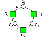
$$,\quad\Gamma =\begin{cases}G=\begin{cases}G_{1}=|1_{1}0_{6}\rangle+|0_{1}1_{6}\rangle+|1_{1}1_{6}\rangle~{},&\text{clause $(x_{1}\vee x_{2})$}\\ G_{2}=|1_{2}0_{3}\rangle+|0_{2}1_{3}\rangle+|1_{2}1_{3}\rangle~{},&\text{clause $(x_{2}\vee x_{3})$}\\ G_{3}=|1_{4}0_{5}\rangle+|0_{4}1_{5}\rangle+|1_{4}1_{5}\rangle~{},&\text{clause $(x_{1}\vee x_{3})$}\end{cases}\\ C=\begin{cases}{C}_{1}=\langle 0_{5}0_{6}|+\langle 1_{5}1_{6}|~{},&\hskip 38.0pt\text{variable $x_{1}$}\\ {C}_{2}=\langle 0_{1}0_{2}|+\langle 1_{1}1_{2}|~{},&\hskip 38.0pt\text{variable $x_{2}$}\\ {C}_{3}=\langle 0_{3}0_{4}|+\langle 1_{3}1_{4}|~{},&\hskip 38.0pt\text{variable $x_{3}$}\end{cases}\\ E=\{1,\ldots,6\}~{}.\end{cases}$$

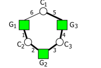
$$,\quad\quad\quad\underbrace{G_{2}\Big{(}C_{2}\big{(}G_{1}\big{)},C_{3}\big{(}G_{3}(C_{1})\big{)}\Big{)}}_{\text{Cayley/Dyck/Newick format}} \Longrightarrow$$

$$\quad\quad\quad\quad\quad\quad G_{2}\otimes C_{2}\otimes G_{1}\otimes C_{3}\otimes G_{3}\otimes C_{1} =val(\Gamma)~{}.$$

Figure 1: The tensor contraction network $\Gamma$ associated with boolean formula Eq. 1 (top). A minimum spanning tree $T$ rooted at $G_{2}$, and the corresponding Newick format (bottom).

We claim that the $val(\Gamma)=4$, which is the number of satisfying solutions to the Boolean formula in Eq. 1. We first examine the cogates $C_{1},C_{2},C_{3}$. Observe that the bra $\langle 00|+\langle 11|$ forces the state of the incident edges to be either all zero ($\langle 0|$) or all one ($\langle 1|$). This is combinatorially analogous to the fact that if a variable is set to false in a clause, then it is false everywhere in the Boolean formula (and similarly for true). We now examine gates $G_{1},G_{2},G_{3}$. The only kets that exist in these gates are kets consistent with a standard OR operation. For example, $|10\rangle,|01\rangle$ or $|11\rangle$. As we compute the tensor contraction of $\Gamma$, we will see that the contractions of bras and kets that are performed represent a brute-force iteration over every possible solution, and the only contractions $\langle x|y\rangle$ that equal one (and are thus “counted”) correspond to legitimate solutions.

We first compute $val(\Gamma)$ via a standard exponential-time algorithm. In Step 1, we arbitrarily choose a root of $\Gamma$, and compute a minimum spanning tree. In Step 2, we represent the minimum spanning tree in Cayley/Dyck/Newick format. In Step 3, we perform the contraction according to the order defined by the Newick tree representation.

In Fig. 1 (bottom), we demonstrate a minimum spanning tree of $\Gamma$ with $G_{2}$ as the root, and the corresponding nested Newick [cite_newick] format which defines the order of the contraction. We now calculate $val(\Gamma)$.

$$G_{3}\otimes C_{1} =\big{(}|1_{4}0_{5}\rangle+|0_{4}1_{5}\rangle+|1_{4}1_{5}\rangle\big{)}\otimes\big{(}\langle 0_{5}0_{6}|+\langle 1_{5}1_{6}|\big{)}=\langle 0_{6}|1_{4}\rangle+\langle 1_{6}|0_{4}\rangle+\langle 1_{6}|1_{4}\rangle~{}.$$

$${C}_{3}\otimes G_{3}\otimes C_{1} =\big{(}\langle 0_{3}0_{4}|+\langle 1_{3}1_{4}|\big{)}\otimes\big{(}\langle 0_{6}|1_{4}\rangle+\langle 1_{6}|0_{4}\rangle+\langle 1_{6}|1_{4}\rangle\big{)}~{}=\langle 0_{3}1_{6}|+\langle 1_{3}0_{6}|+\langle 1_{3}1_{6}|~{}.$$

$$G_{2}\otimes C_{2}\otimes G_{1}\otimes C_{3}\otimes G_{3}\otimes C_{1} =\mathbf{4}~{}.$$

By inspecting the intermediary steps, we see that the individual bra-ket contractions performed throughout the calculation are essentially a brute-force iteration over all the possible true-false assignments to the variables in the original Boolean formula. Thus, it is clear that processing the contraction in this way takes exponential time.

We will now present an alternative, polynomial-time computable method for calculating $val(\Gamma)$. First we recall the direct sum (denoted $\oplus$) of two labeled matrices. In order to describe the labeling method of the rows and columns, recall that in a tensor contraction network, every gate or cogate is an element of a tensor product space as defined by the incident edges. For example, in Fig. 1, observe that cogate $C_{3}$ is incident on edges 3 and 4, and $C_{3}=\langle 0_{3}0_{4}|+\langle 1_{3}1_{4}|\in V^{*}_{3}\otimes V^{*}_{4}$. Since cogate $C_{3}$ is Pfaffian (see Ex. 3), there exists a matrix $\Theta$ and a scalar $\beta$ such that $\beta\hskip 1.0pt\text{sPf}^{*}(\Theta)=\langle 0_{3}0_{4}|+\langle 0_{3}0_{4}|$. In this case, $\Theta$ is a $2\times 2$ matrix (since $C_{3}$ is a 2-arity cogate), and the rows and columns of $\Theta$ are labeled with edges $3$ and $4$:

$$\hbox{}\;\vbox{\kern 28.46666pt\hbox{$\kern 62.22226pt\kern-4.75pt\left[\kern-62.22226pt\vbox{\kern-28.46666pt\vbox{\halign{$#$\hfil\kern 2\p@\kern\@tempdima&\thinspace\hfil$#$\hfil&&\quad\hfil$#$\hfil\cr\hfil\crcr\kern-12.0pt\cr$\hfil\kern 2.0pt\kern 4.75pt&3&4\crcr\kern 2.0pt\cr 3$\hfil\kern 2.0pt\kern 4.75pt&0&\frac{\sqrt{5}}{2}+\frac{3}{2}\cr 4$\hfil\kern 2.0pt\kern 4.75pt&-\big{(}\frac{\sqrt{5}}{2}+\frac{3}{2}\big{)}&0\cr\cr}}\kern-12.0pt}\,\right]$}}~{}.$$

Now consider a tensor contraction network $\Gamma=\{G,C,E\}$ with all gates/cogates Pfaffian, and let $\{\Xi_{1},\ldots,\Xi_{|G|}\}$ be the set of matrices associated with the Pfaffian gates $G=\{G_{1},\ldots,G_{|G|}\}$ (note that no cogates are included). Since $\Gamma$ is a bipartite graph, the row and column labels associated with any two $\Xi,\Xi^{\prime}\in\{\Xi_{1},\ldots,\Xi_{|G|}\}$ are disjoint. Let $I$ be the set of row/column labels of $\Xi$ and $J$ be the set of row/column labels of $\Xi^{\prime}$, and let $\sigma$ be an order on the edges of $\Gamma$. Then the direct sum $\Xi\oplus_{\sigma}\Xi^{\prime}$ is the matrix $\Xi^{\prime\prime}$ with row/column label set $I\cup J$ ordered according to $\sigma$ where $\xi^{\prime\prime}_{k\ell}=0$ if $k\in I$ and $\ell\in J$ or vice versa, $\xi^{\prime\prime}_{k\ell}=\xi_{k\ell}$ if $k,\ell\in I$, and $\xi^{\prime\prime}_{k\ell}=\xi^{\prime}_{k\ell}$ if $k,\ell\in J$. For example,

$$\underbrace{\bordermatrix{&4&5&6\cr 4&\xi_{44}&\xi_{45}&\xi_{46}\cr 5&\xi_{54}&\xi_{55}&\xi_{56}\cr 6&\xi_{64}&\xi_{65}&\xi_{66}\cr}}_{\Xi}\quad\oplus_{\sigma}\quad\underbrace{\bordermatrix{&1&3&8&9\cr 1&\xi^{\prime}_{11}&\xi^{\prime}_{13}&\xi^{\prime}_{18}&\xi^{\prime}_{19}\cr 3&\xi^{\prime}_{31}&\xi^{\prime}_{33}&\xi^{\prime}_{38}&\xi^{\prime}_{39}\cr 8&\xi^{\prime}_{81}&\xi^{\prime}_{83}&\xi^{\prime}_{88}&\xi^{\prime}_{89}\cr 9&\xi^{\prime}_{91}&\xi^{\prime}_{93}&\xi^{\prime}_{98}&\xi^{\prime}_{99}}}_{\Xi^{\prime}}\quad=\quad\underbrace{\bordermatrix{&1&3&4&5&6&8&9\cr 1&\xi^{\prime}_{11}&\xi^{\prime}_{13}&0&0&0&\xi^{\prime}_{18}&\xi^{\prime}_{19}\cr 3&\xi^{\prime}_{31}&\xi^{\prime}_{33}&0&0&0&\xi^{\prime}_{38}&\xi^{\prime}_{39}\cr 4&0&0&\xi_{44}&\xi_{45}&\xi_{46}&0&0\cr 5&0&0&\xi_{54}&\xi_{55}&\xi_{56}&0&0\cr 6&0&0&\xi_{64}&\xi_{65}&\xi_{66}&0&0\cr 8&\xi^{\prime}_{81}&\xi^{\prime}_{83}&0&0&0&\xi^{\prime}_{88}&\xi^{\prime}_{89}\cr 9&\xi^{\prime}_{91}&\xi^{\prime}_{93}&0&0&0&\xi^{\prime}_{98}&\xi^{\prime}_{99}}}_{\Xi\oplus_{\sigma}\Xi^{\prime}=\Xi^{\prime\prime}}$$

The Pfaffian circuit evaluation theorem relies on the planar spanning tree edge order.

(a)

(b)

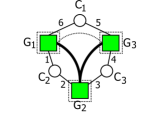
(c)

(d)

Figure 2: Finding the planar spanning tree edge order.

In order to the find the planar spanning tree edge order, we follow the four steps demonstrated in Fig. 2. Given a tensor contraction network $\Gamma$, for each interior face, we connect the gates incident on that interior face in a cycle (Fig. 2.a). Next, we take a spanning tree of the edges in those cycles (Fig. 2.b), and draw “boxes” around each of the gates (Fig. 2.c). Finally, we trace the spanning tree from gate to gate, following the “boxes” around the gates (Fig. 2.d). This creates a closed curve that crosses every edge exactly once. Then, we trace the curve, beginning at any point, and tracing in any direction, ordering the edges according to when they are crossed by the curve. For example, in Fig. 2.d, if we begin at $G_{1}$ where the curve crosses between gate $G_{1}$ and cogate $C_{2}$, and trace in counter-clockwise order. This yields the very convenient edge order $\{1,2,3,4,5,6\}$. The planar spanning tree edge order is discussed in detail in [morton_pfaff].

The following lemma is the first part of the Pfaffian circuit evaluation theorem.

Lemma 1 ([morton_pfaff]).

Let $\Gamma$ be a planar tensor contraction network of Pfaffian gates and cogates and let $\sigma$ be a planar spanning tree edge order. Let $G_{1},\ldots,G_{|G|}$ be the Pfaffian gates with $G_{i}=\alpha_{i}\hskip 1.0pt\text{sPf}(\Xi_{i})$ for $1\leq i\leq|G|$. Then

$$G_{1}\otimes\cdots\otimes G_{|G|}=\big{(}\alpha_{1}\cdots\alpha_{|G|}\big{)}\hskip 2.0pt\text{\emph{sPf}}\big{(}\Xi_{1}\oplus_{\sigma}\cdots\oplus_{\sigma}\Xi_{|G|}\big{)}~{}.$$ (2)

The analogous result holds for cogates.

Observe that both sides of Eq. 2 require exponential time to evaluate. However, the direct sum $\Xi_{1}\oplus_{\sigma}\cdots\oplus_{\sigma}\Xi_{|G|}$ can be calculated in polynomial-time. We now combine the gate and cogate versions of Lemma 1 to state the Pfaffian circuit evaluation theorem.

Theorem 1 (Pfaffian circuit evaluation theorem, [morton_pfaff]).

Given a planar, Pfaffian tensor contraction network with an even number of edges and an edge order $\sigma$, let $\Xi_{1},\ldots,\Xi_{|G|}$ (and $\Theta_{1},\ldots,\Theta_{|C|}$, respectively) be the matrices from Lemma 1. Furthermore, let $\Xi=\Xi_{1}\oplus_{\sigma}\cdots\oplus_{\sigma}\Xi_{|G|}$, and $\Theta=\Theta_{1}\oplus_{\sigma}\cdots\oplus_{\sigma}\Theta_{|C|}$. Let $\widetilde{\Theta}$ be $\Theta$ with the signs flipped such that $\widetilde{\theta}_{ij}=(-1)^{i+j+1}\theta_{ij}$. Then

$$\underbrace{\big{\langle}\beta\hskip 1.0pt\text{\emph{sPf}}^{*}(\widetilde{\Theta})~{}|~{}\alpha\hskip 1.0pt\text{\emph{sPf}}(\Xi)\big{\rangle}}_{\text{exponential-time}} =\underbrace{\alpha\beta\hskip 1.0pt\text{\emph{Pf}}(\widetilde{\Theta}+\Xi)}_{\text{polynomial-time}}~{}.$$ (3)

Observe that the left-hand side of Eq. 3 requires exponential-time to compute, since it involves the contraction of every bra/ket in the subPfaffian/subPfaffian dual. However, the right-hand side has the same complexity as the determinant of an $m\times m$ matrix (where $\Gamma$ has $m$ edges), and is thus computable in polynomial-time in the size of $\Gamma$. To conclude our example, let

$$k =\frac{5^{1/2}}{2}+\frac{3}{2}~{},\quad\quad\text{and let}\quad A=\left[\begin{array}[]{cc}\frac{1}{10}\big{(}-5^{3/4}+5^{5/4})&5^{-1/4}\\ \frac{1}{10}\big{(}-5^{3/4}-5^{5/4}\big{)}&5^{-1/4}\end{array}\right]~{}.$$

Observe that, via Ex. 3 and Fig. 1, $\Gamma$ is Pfaffian under the homogeneous change of basis $A$. Then, via Lemma 1 and Ex. 3, we see representations for $G_{2}\otimes G_{1}\otimes G_{3}$ and $C_{1}\otimes C_{2}\otimes C_{3}$:

$$(A\oplus A)(G_{2}\otimes G_{1}\otimes G_{3}) =\text{sPf}(\underbrace{\Xi_{2}\oplus_{\sigma}\Xi_{1}\oplus_{\sigma}\Xi_{3}}_{\Xi})~{},$$

$$(A^{-1}\oplus A^{-1})C_{1}\otimes C_{2}\otimes C_{3} =\beta^{3}\text{sPf}^{*}(\underbrace{\Theta_{1}\oplus_{\sigma}\Theta_{2}\oplus_{\sigma}\Theta_{3}}_{\Theta})~{}.$$

Therefore,

$$\overbrace{\bordermatrix{\text{}&2&3\cr 2&0&-1\cr 3&1&0}}^{\Xi^{G}_{2}}\quad\oplus_{\sigma}\quad\overbrace{\bordermatrix{\text{}&1&6\cr 1&0&-1\cr 6&1&0}}^{\Xi^{G}_{1}}\quad\oplus_{\sigma}\quad\overbrace{\bordermatrix{\text{}&4&5\cr 4&0&-1\cr 5&1&0}}^{\Xi^{G}_{3}}\quad=\quad\bordermatrix{\text{}&1&2&3&4&5&6\cr 1&0&0&0&0&0&-1\cr 2&0&0&-1&0&0&0\cr 3&0&1&0&0&0&0\cr 4&0&0&0&0&-1&0\cr 5&0&0&0&1&0&0\cr 6&1&0&0&0&0&0}\quad\text{and~{},}$$

$$\overbrace{\bordermatrix{\text{}&1&2\cr 1&0&k\cr 2&-k&0}}^{\Theta_{1}}\quad\oplus_{\sigma}\quad\overbrace{\bordermatrix{\text{}&3&4\cr 3&0&k\cr 4&-k&0}}^{\Theta_{2}}\quad\oplus_{\sigma}\quad\overbrace{\bordermatrix{\text{}&5&6\cr 5&0&k\cr 6&-k&0}}^{\Theta_{3}}\quad=\quad\underbrace{\bordermatrix{\text{}&1&2&3&4&5&6\cr 1&0&k&0&0&0&0\cr 2&-k&0&0&0&0&0\cr 3&0&0&0&k&0&0\cr 4&0&0&-k&0&0&0\cr 5&0&0&0&0&0&k\cr 6&0&0&0&0&-k&0}}_{\Theta}\quad\phantom{\text{and~{}}}.$$

Finally, we see

$$\widetilde{\Theta}+\Xi =\bordermatrix{\text{}&1&2&3&4&5&6\cr 1&0&k&0&0&0&-1\cr 2&-k&0&-1&0&0&0\cr 3&0&1&0&k&0&0\cr 4&0&0&-k&0&-1&0\cr 5&0&0&0&1&0&k\cr 6&1&0&0&0&-k&0}\Longrightarrow$$

$$\text{Pf}\big{(}\widetilde{\Theta}+\Xi\big{)} =8+4\sqrt{5}~{},$$

$$\beta^{3}\text{Pf}\big{(}\widetilde{\Theta}+\Xi\big{)} =\bigg{(}\frac{\sqrt{5}}{2}-\frac{1}{2}\bigg{)}^{3}\big{(}8+4\sqrt{5}\big{)}~{},$$

$$=\mathbf{4}~{}.$$

Thus, $val(\Gamma)$, as calculated by the Pfaffian circuit evaluation theorem, is equal to the number of satisfying solutions to the underlying combinatorial problem. We conclude by mentioning that if the number of edges in $\Gamma$ is odd, then $\text{Pf}(\widetilde{\Theta}+\Xi)=0$, and there is no relation between the Pfaffian and $val(\Gamma)$. This explains why the Pfaffian circuit evaluation theorem only applies to planar, Pfaffian circuits with an even number of edges (see [morton_pfaff] for more detail).

3 Constructing Pfaffian Circuits via Algebraic Methods

A gate is Pfaffian (after a heterogeneous change of basis) if there exists an $n\times n$ skew-symmetric matrix $\Xi$, an $\alpha\in\mathbb{C}$, and matrices $A_{1},\ldots,A_{n}\in\mathbb{C}^{2\times 2}$ such that $(A_{1}\otimes\cdots\otimes A_{n})G=\alpha\hskip 1.0pt\text{sPf}(\Xi)$ (Def. 2). In this section, we present an algebraic model of this property. In other words, given a gate $G$ (or cogate $C$), we present a system of polynomial equations such that the changes of bases $A_{1},\ldots,A_{n}$ under which $G$ is Pfaffian are in bijection to the solutions of this system. If there are no solutions, then there do not exist any matrices $A_{1},\ldots,A_{n}$ such that $(A_{1}\otimes\cdots\otimes A_{n})G=\alpha\hskip 1.0pt\text{sPf}(\Xi)$, and $G$ is not Pfaffian. We comment that there is a wealth of literature on pursuing combinatorial problems via systems of polynomial equations (see [alonsurvey, alontarsi, susan_cpc, lovasz1, onn] and references therein).

Throughout the rest of this paper, in order to prove that a given gate/cogate is Pfaffian, we simply demonstrate the $n\times n$ skew-symmetric matrix $\Xi$, the scalar $\alpha$, and the change of basis matrices $A_{1},\ldots,A_{n}$ such that $G$ is Pfaffian, without further explanation. But we observe in advance that all such “Pfaffian certificates” (i.e., those displayed in Ex. 3) are found via solving the system of equations presented below. When we state that a given gate/cogate is not Pfaffian, we specifically mean that the Gröbner basis of the system of polynomial equations described below (found via computation with Singular) consists of the single polynomial 1. Thus, the variety associated with the ideal is empty, and there are no solutions.

Before presenting the system of polynomial equations, we introduce the following notation. Let $[n]$ denote the set of integers $\{1,\ldots,n\}$. Given an integer $i\in[n]$ and a set $I\subseteq[n]$, the notation $I_{i}\in\{0,1\}$ denotes the $i$-th bit of the bitstring representation of $I$. For example, given $I=\{1,3\}\subseteq[4]$, then $|I\rangle$ is equivalent to $|1010\rangle$, with $I_{1}=1,I_{2}=0,I_{3}=1$ and $I_{4}=0$. Given an $n$-arity gate $G=\sum_{I\subseteq[n]}G_{I}|I\rangle$, let $G^{\prime}=(A_{1}\otimes\cdots\otimes A_{n})G$, and then the following formula defines the coefficient $G^{\prime}_{I^{\prime}}$ where $I^{\prime}\subseteq[n]$:

$$G^{\prime}_{I^{\prime}} =\sum_{I\subseteq[n]}G_{I}\prod_{i=1}^{n}A_{i}[I^{\prime}_{i},I_{i}]~{}.$$ (4)

Example 4.

Let $A$ be the matrix below and consider a generic 3-arity gate $G$:

$$A=\left[\begin{array}[]{cc}a_{00}&a_{01}\\[-4.30554pt] a_{10}&a_{11}\end{array}\right]~{},\quad\quad$$

$$G =G_{000}|000\rangle+G_{010}|010\rangle+G_{001}|001\rangle+G_{011}|011\rangle+G_{100}|100\rangle$$

$$\phantom{=~{}}+G_{110}|110\rangle+G_{101}|101\rangle+G_{111}|111\rangle~{}.$$

Then, given $G^{\prime}=A^{\otimes 3}G$, the coefficient of the ket $|100\rangle$ in $G^{\prime}$, denoted $G^{\prime}_{100}$, is

$$G^{\prime}_{100} =G_{000}a_{10}a_{00}^{2}+G_{100}a_{11}a_{00}^{2}+G_{010}a_{10}a_{01}a_{00}+G_{001}a_{10}a_{00}a_{01}+G_{110}a_{11}a_{01}a_{00}$$

$$\phantom{=}+G_{101}a_{11}a_{00}a_{01}+G_{011}a_{10}a_{01}^{2}+G_{111}a_{11}a_{01}^{2}~{}.$$

$\Box$

Finally, given $I\subseteq[n]$ with $|I|$ even and $|I|\geq 4$, let $I_{\min}$ be the smallest integer in $I$.

Theorem 2.

Let $G=\sum_{I\subseteq[n]}G_{I}|I\rangle$ be an $n$-arity gate, and let $G^{\prime}=(A_{1}\otimes\cdots\otimes A_{n})G$ with $G^{\prime}_{I^{\prime}}$ defined by Eq. 4. Then, the solutions to the following system of polynomial equations are in bijection to the changes of bases $A_{1},\ldots,A_{n}$ such that $G$ is Pfaffian.

$$\big{(}G^{\prime}_{\emptyset}\big{)}^{-1}{G^{\prime}}_{I^{\prime}} =0,\hskip 148.0pt\text{~{}$\forall$ $I^{\prime}\subseteq[n]$ with $|I^{\prime}|$ odd}~{},$$ (5)

$$\big{(}G^{\prime}_{\emptyset}\big{)}^{-1}{G^{\prime}}_{I^{\prime}} =\sum_{i\in{I^{\prime}}\setminus{I^{\prime}}_{\min}}(-1)^{{I^{\prime}}_{\min}+i+1}\Big{(}\big{(}G^{\prime}_{\emptyset}\big{)}^{-1}\Big{)}^{2}G^{\prime}_{{I^{\prime}}_{\min},i}{G^{\prime}}_{{I^{\prime}}\setminus\{{I^{\prime}}_{\min},i\}}~{},$$

$$\hskip 105.0pt\text{~{}$\forall$ $I^{\prime}\subseteq[n]$ with $|I^{\prime}|$ even and $|I^{\prime}|\geq 4$}~{},$$ (6)

$$\sum_{I\subseteq[n]}G_{I}\prod_{i=1}^{n}A_{i}[0,I_{i}]-G^{\prime}_{\emptyset} =0~{},$$ (7)

$$G^{\prime}_{\emptyset}\big{(}G^{\prime}_{\emptyset}\big{)}^{-1}-1=0~{},$$ (8)

$$\det(A_{i})\big{(}\det(A_{i})\big{)}^{-1}-1 =0,\text{~{}for~{}$1\leq i\leq n$}~{},$$ (9)

We refer to Eqs. 8 and 9 as the “inversion” equations, since Eq. 9 insures that each of the matrices $A_{1},\ldots,A_{n}$ are invertible, and Eq. 8 insures that the coefficient for $G^{\prime}_{\emptyset}$ can be scaled to equal one (since the Pfaffian of the empty matrix is equal to one by definition). This scaling factor appears again in Eqs. 5 and 6, taking into account that each coefficient $G^{\prime}_{I^{\prime}}$ is scaled by $\alpha$ since $(A_{1}\otimes\cdots\otimes A_{n})G=\alpha\hskip 1.0pt\text{sPf}(\Xi)$. Eq. 7 is simply the equation for $G^{\prime}_{\emptyset}$ according to the change of basis formula given in Eq. 4. We refer to Eqs. 5 and 6 as the “parity” and “consistency” equations, respectively. The parity equations capture the condition that the Pfaffian of an $n\times n$ matrix with $n$ odd is zero. To understand the “consistency” equations, recall that the Pfaffian of a given $n\times n$ matrix with $n$ even can be recursively written in terms the Pfaffians of each of the $(n-1)\times(n-1)$ submatrices. For example, the Pfaffian of $6\times 6$ matrix $A$ can be expressed as $a_{12}\text{Pf}(A|_{3456})-a_{13}\text{Pf}(A|_{2456})+a_{14}\text{Pf}(A|_{2356})-a_{15}\text{Pf}(A|_{2346})+a_{16}\text{Pf}(A|_{2345})$. In this case, observe that $I^{\prime}=\{1,2,3,4,5,6\}$, and $I^{\prime}_{\min}=1$. Though Theorem 2 refers gates, there is an analogous theorem for cogates.

Example 5.

Let $G=\text{OR}=|10\rangle+|01\rangle+|11\rangle$, and let $G^{\prime}=(A\otimes B)G$. Then, the system of equations associated with Theorem 2 is as follows:

$$\big{(}{G^{\prime}}_{\emptyset}\big{)}^{-1}(a_{11}b_{00}+a_{10}b_{01}+a_{11}b_{01})=\big{(}{G^{\prime}}_{\emptyset}\big{)}^{-1}(a_{01}b_{10}+a_{00}b_{11}+a_{01}b_{11})=0~{},$$

$$a_{01}b_{00}+a_{00}b_{01}+a_{01}b_{01}-{G^{\prime}}_{\emptyset}=a_{00}a_{11}-a_{01}a_{10}-\det(A)=b_{00}b_{11}-b_{01}b_{10}-\det(B)=0~{},$$

$${G^{\prime}}_{\emptyset}\big{(}{G^{\prime}}_{\emptyset}\big{)}^{-1}-1=0~{},\quad\det(A)\big{(}\det(A)\big{)}^{-1}-1=0~{},\quad\det(B)\big{(}\det(B)\big{)}^{-1}-1=0~{}.$$

Note that the change of basis in Ex. 3 is indeed a solution to this system of equations.

The next two sections detail the results of computing with these algebraic models.

4 Boolean Variables and Tensor Contraction Networks

In the field of combinatorial optimization, there are an almost countless number of problems (independent set, dominating set, bin packing, partition, satisfiability, etc.) that can be modeled as a series of equations in which the variables are restricted to 0/1 values (also called binary or Boolean variables). In a generalized counting constraint satisfaction setting, we cannot assume that we are allowed to swap variables or copy them (indeed the latter is impossible in the quantum setting). Thus to demonstrate the applicability of Pfaffian circuits to 0/1 #CSP problems, we must first demonstrate a planar, Pfaffian tensor representation of a variable that is either zero or one in every constraint where it appears. Such a tensor may only be avaiable for restricted arities; hence the popularity of restrictions such as “read-twice” in the literature on holographic algorithms. In this section, we explore two different representations of Boolean variables, the first utilizing a homogeneous change of basis, and the second possible under a heterogeneous change of basis only. We compare and contrast these two constructions, focusing in particular on categorizing the gates/cogates that pair with these representations, since these collections represent a class of 0/1 #CSP problems solvable in polynomial time.

In order to model a 0/1 #CSP problem as a tensor contraction network, we first recall the standard variable/constraint graph (see Fig. 3.a), which is a bipartite graph with variables above and constraints below, and an edge between a variable and constraint if a given variable appears in a particular constraint. In order to translate this graph to a Pfaffian circuit, we simply model variables as cogates and constraints as gates (see Fig. 3.b), or vice versa.

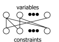
(a)

(b)

Figure 3: Variable/constraint graph as a tensor contraction network.

Following the graphs presented in Fig. 3, we need a tensor that models the property that if a variable is set to zero, it is simultaneously zero in every constraint in which it appears (and similarly for one). The obvious suggestion for modeling a Boolean variable as a tensor is the following gate or cogate, commonly denoted as the equal gate/cogate:

$$|00\cdots 0\rangle+|11\cdots 1\rangle~{},\quad\quad\langle 00\cdots 0|+\langle 11\cdots 1|~{}.$$

Consider the gate $|0\cdots 0\rangle+|1\cdots 1\rangle$. If any edge is set to $|0\rangle$, then every edge is set to $|0\rangle$, and similarly for $|1\rangle$ (see Ex. 6). Observe that gate $(|0\rangle+|1\rangle)^{\otimes n}$ does not satisfy this property.

Example 6.

Consider the following tensor contraction network fragment, containing gate $G_{1}$ and cogates $C_{1}$ and $C_{2}$, where edges $1,\ldots,6$ are labeled, and $7,\ldots,m$ are unlabeled.

$$G_{1} =|0_{1}0_{4}\cdots 0_{m}\rangle+|1_{1}1_{4}\cdots 1_{m}\rangle~{},$$

$$C_{1} =\langle 0_{1}0_{2}1_{3}|+\langle 0_{1}1_{2}0_{3}|+\langle 0_{1}1_{2}1_{3}|~{},$$

$$C_{2} =\langle 0_{4}1_{5}1_{6}|+\langle 1_{4}0_{5}0_{6}|~{}.$$

While computing $val(\Gamma)$, the contraction $C_{1}\otimes G_{1}$ is performed:

$$\Big{\langle}\big{(}\langle 0_{1}0_{2}1_{3}|+\langle 0_{1}1_{2}0_{3}|+\langle 0_{1}1_{2}1_{3}|\big{)}\Big{|}\big{(}|0_{1}0_{4}\cdots 0_{m}\rangle+|1_{1}1_{4}\cdots 1_{m}\rangle\big{)}\Big{\rangle}~{}.$$

Since $\langle 0_{1}|1_{1}\rangle=0$, the partial contraction $\Big{\langle}\langle 0_{1}0_{2}1_{3}|+\langle 0_{1}1_{2}0_{3}|+\langle 0_{1}1_{2}1_{3}|\Big{|}|1_{1}1_{4}\cdots 1_{m}\rangle\Big{\rangle}~{}=~{}0$. Therefore, the only non-zero terms arise from $\Big{\langle}\big{(}\langle 0_{1}0_{2}1_{3}|+\langle 0_{1}1_{2}0_{3}|+\langle 0_{1}1_{2}1_{3}|\big{)}\Big{|}\big{(}|0_{1}0_{4}\cdots 0_{m}\rangle\big{)}\Big{\rangle}$, since $\langle 0_{1}|0_{1}\rangle=1$. Thus, even though cogate $C_{2}$ contains bra $\langle 1_{4}0_{5}0_{6}|$, that combination is not counted as a solution since $\langle 1_{4}0_{5}0_{6}|0_{1}0_{4}\cdots 0_{m}\rangle=0$. Thus, for any tensor contraction network containing $G_{1}$ (or a similar boolean tensor), if any edge of $G_{1}$ is set to $|0\rangle$ (or $|1\rangle$), all the edges of $G_{1}$ are set to $|0\rangle$ (or $|1\rangle$, respectively). $\Box$

Throughout this section, we refer to $|00\cdots 0\rangle+|11\cdots 1\rangle$ as the n-arity equal gate (or cogate, respectively). The following is a variant of the Hadamard basis of [valiant_qc].

Proposition 1.

The $n$-arity equal gate (or cogate, respectively) is Pfaffian under the homogeneous change of basis $(A\otimes\cdots\otimes A)$ (or $(B^{-1}\otimes\cdots\otimes B^{-1})$, respectively).

$$A=\left[\begin{array}[]{cc}1&1\\[-4.30554pt] 1&-1\end{array}\right]$$

$$,~{}\text{and}~{}B=\left[\begin{array}[]{cc}1&-1\\[-4.30554pt] 1/2&1/2\end{array}\right]~{},~{}B^{-1}=\left[\begin{array}[]{cc}1/2&1\\[-4.30554pt] -1/2&1\end{array}\right]~{},$$

Proof..

We provide a generalized form for the matrices $\Xi$ and $\Theta$ in the “Pfaffian certificates” $(A\otimes\cdots\otimes A)\big{(}|00\cdots 0\rangle+|11\cdots 1\rangle\big{)}=2\hskip 1.0pt\text{sPf}(\Xi)$ and $(B^{-1}\otimes\cdots\otimes B^{-1})\big{(}\langle 00\cdots 0|+\langle 11\cdots 1|\big{)}=2\hskip 1.0pt\text{sPf}^{*}(\Theta)$.

$$(A\otimes\cdots\otimes A)\big{(}|00\cdots 0\rangle+|11\cdots 1\rangle\big{)} =2\hskip 1.0pt\text{sPf}\left(\left[{\begin{array}[]{ccccc}0&1&\cdots&\cdots&1\\[-6.45831pt] -1&0&1&\cdots&1\\[-6.45831pt] \vdots&-1&\ddots&\ddots&\vdots\\[-6.45831pt] \vdots&&\ddots&0&1\\[-6.45831pt] -1&-1&\cdots&-1&0\end{array}}\right]\right)~{},$$

$$(B^{-1}\otimes\cdots\otimes B^{-1})\big{(}\langle 00\cdots 0|+\langle 11\cdots 1|\big{)} =2\hskip 1.0pt\text{sPf}^{*}\left(\left[{\begin{array}[]{ccccc}0&1/4&\cdots&\cdots&1/4\\[-6.45831pt] -1/4&0&1/4&\cdots&1/4\\[-6.45831pt] \vdots&-1/4&\ddots&\ddots&\vdots\\[-6.45831pt] \vdots&&\ddots&0&1/4\\[-6.45831pt] -1/4&-1/4&\cdots&-1/4&0\end{array}}\right]\right)~{}.$$

$\Box$

We now introduce a tensor contraction network fragment that is equivalent to the $n$-arity equal gate/cogate, in that if any edge in the fragment is fixed to $|0\rangle$ or $|1\rangle$, then every edge in the fragment is automatically fixed to the same state. In the following theorem, every vertex is associated with a equal tensor (i.e., the 2-arity cogate is $\langle 00|+\langle 11|$, and the 3-arity gate is $|000\rangle+|111\rangle$, etc.).

Theorem 3.

      

1. There does not exist a matrix $A\in\mathbb{C}^{2\times 2}$ such that the collection of equal gates/cogates in Fig. 4.a are Pfaffian under the change of basis $A$.

2. There do exist matrices $A,B\in\mathbb{C}^{2\times 2}$ such that the collection of equal gates/cogates in Fig. 4.b are Pfaffian under the changes of bases $A$ and $B$.

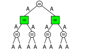
(a)

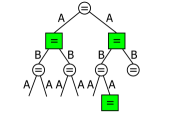
(b)

Figure 4: Boolean trees (homogeneous and heterogeneous)

Proof..

The proof of Theorem 3.1 is by a Gröbner basis computation that runs in under a second. For Theorem 3.2, we present the “Pfaffian certificates” for each of the equal gates/cogates present in the Boolean tree. Let $A,B\in\mathbb{C}^{2\times 2}$ be as follows:

$$A=\left[\begin{array}[]{cc}1&1\\[-6.45831pt] 1&-1\end{array}\right]~{},\quad A^{-1}=-\frac{1}{2}\left[\begin{array}[]{cc}-1&-1\\[-6.45831pt] -1&1\end{array}\right]~{},\quad B=\left[\begin{array}[]{cc}1&-1\\[-6.45831pt] 1/2&1/2\end{array}\right]~{},\quad B^{-1}=\left[\begin{array}[]{cc}1/2&1\\[-6.45831pt] -1/2&1\end{array}\right]~{},$$

$$\big{(}A^{-1}\otimes A^{-1}\big{)}\big{(}\langle 00|+\langle 11|\big{)} =\frac{1}{2}\hskip 1.0pt\text{sPf}^{*}\left(\left[\begin{array}[]{cc}0&1\\[-6.45831pt] -1&0\end{array}\right]\right)~{},$$

$$(A\otimes B\otimes B)\big{(}|000\rangle+|111\rangle\big{)} =2\hskip 1.0pt\text{sPf}\left(\left[\begin{array}[]{ccc}0&1/2&1/2\\[-6.45831pt] -1/2&0&1/4\\[-6.45831pt] -1/2&-1/4&0\end{array}\right]\right)~{},$$

$$\big{(}B^{-1}\otimes A^{-1}\otimes A^{-1}\big{)}\big{(}\langle 000|+\langle 111|\big{)} =\frac{1}{2}\hskip 1.0pt\text{sPf}^{*}\left(\left[\begin{array}[]{ccc}0&1/2&1/2\\[-6.45831pt] -1/2&0&1\\[-6.45831pt] -1/2&-1&0\end{array}\right]\right)~{},$$

$$B^{-1}\big{(}\langle 0|+\langle 1|\big{)}=2\hskip 1.0pt\text{sPf}^{*}\left(\left[\begin{array}[]{c}0\end{array}\right]\right)~{}, \quad A\big{(}|0\rangle+|1\rangle\big{)}=2\hskip 1.0pt\text{sPf}\left(\left[\begin{array}[]{c}0\end{array}\right]\right)~{}.$$

$\Box$

We will refer to the trees defined by Theorem 3.2 as Boolean trees, since they are meant to represent 0/1 variables or $n$-arity equal gates/cogates. We first observe that these trees can be extended to an arbitrary height. Since the gates ($\Box$) are Pfaffian under the change of basis $A,BB$, and the cogates ($\circ$) are Pfaffian under the change of basis $B,AA$, the gates can always be connected to the cogates, and vice versa, allowing the tree to be indefinitely “grown”. We next observe that any gate can be “sealed off” with the 1-arity Boolean cogate $\langle 0|+\langle 1|$ (which is Pfaffian under change of basis $B$), and that any cogate can likewise be “sealed off” with the 1-arity Boolean gate $|0\rangle+|1\rangle$ (which is Pfaffian under the change of basis $A$). Therefore, for any integer $n$, there exists a Boolean tree that is equivalent to an $n$-arity Boolean gate/cogate. For example, Fig. 4.b is equivalent to 5-arity Boolean cogate.

One metric of comparison for Boolean trees and $n$-arity Boolean gates/cogates is the complexity of their respective Gröbner bases. For example, the following 18 equations in degrees one, two and three is the Gröbner basis for a Boolean tree of arbitrary size:

$$a_{10}+a_{11}=a_{00}-a_{01}=2a_{11}^{2}-1=2a_{01}a_{11}-\det(A)=2a_{01}^{2}-\det(A)^{2}=0~{},$$

$$a_{01}\det(A)^{-1}-a_{11}=a_{11}\det(A)-a_{01}=\det(A)\det(A)^{-1}-1=0~{},$$

$$b_{10}-b_{11}=b_{00}+b_{01}=2b_{11}-1=b_{01}+\det(B)=\det(B)\det(B)^{-1}-1=0~{},$$

$$\big{(}\det(B)^{-1}\big{)}^{2}-2a_{01}=2a_{11}\det(B)-\det(A)^{-1}\det(B)^{-1}=2a_{01}\det(B)-\det(B)^{-1}=0~{},$$

$$a_{11}\det(A)^{-1}-\det(B)^{2}=2\det(B)^{3}-\big{(}\det(A)^{-1}\big{)}^{2}\det(B)^{-1}=0~{}.$$

By comparison, the Gröbner basis of the 9-arity Boolean cogate contains 82 polynomials, ranging from degrees two to ten. Furthermore, the complexity of the Gröbner basis of the $n$-arity Boolean gate/cogate obviously grows with respect to $n$, while the complexity of the “$n$-arity” Boolean tree remains constant. Since the algebraic approach to exploring Pfaffian circuits relies on the complexity of computing the Gröbner basis, the question of categorizing classes of compatible gates/cogates (representing constraints) is obviously more efficiently pursued with Boolean trees.

Despite the algebraic advantages of using a Boolean tree (as opposed to an $n$-arity equal gate/cogate), at first glance it may seem that introducing two distinct bases $A$ and $B$ may complicate the question of identifying compatible constraint gates/cogates. The two obstacles to overcome are 1) that the overall tensor contraction network must remain bipartite, and 2) that each of the gates/cogates must be simultaneously Pfaffian. However, the following proposition demonstrates that it is possible to treat the bases $A$ and $B$ as virtually interchangeable, since a “bridge” can always be built from gate to cogate, and from basis $A$ to basis $B$ (and vice versa).

Proposition 2.

Given matrices $A,B$ as in Prop. 1, the following 2-arity gates/cogates are Pfaffian under both $(A\otimes A)$ and $(B\otimes B)$: $\langle 00|+\langle 11|,|00\rangle+|11\rangle$ (Equal), and $\langle 10|+\langle 01|,|10\rangle+|01\rangle$ (not) .

Furthermore, the following is a direct corollary of Theorem 3.

Corollary 1.

Given matrices $A,B$ as in Prop. 1, the following two gate/cogate combinations are Pfaffian under the indicated changes of bases.

$\Box$

The significance of Prop. 2 is that a gate can be arbitrarily changed into a cogate, without changing the state on the outgoing edge (equal), or by flipping the state (not) from $|0\rangle$ to $|1\rangle$ (or $\langle 0|$ and $\langle 1|$, respectively). The significance of Cor. 1 is that not only can a gate be changed to a cogate, but the basis on the outgoing edge itself can be changed (from $A$ to $B$, or vice versa) without altering the state on the outgoing edge. We will now investigate how to categorize the gates/cogates that successfully pair with a Boolean tree. Towards that end, we introduce the following definition.

Definition 3.

A gate $G$ is invariant under complement, if for every ket $|I\rangle$ in the tensor $G$, the complement ket $\overline{|I\rangle}$ also appears in the tensor.

Example 7.

Here are two 3-arity gates that are invariant under complement:

$$|010\rangle+|001\rangle+|110\rangle+|101\rangle~{}, \quad|100\rangle+|001\rangle+|110\rangle+|011\rangle~{}.$$

Theorem 4.

Given matrices $A,B$ as in Prop. 1, then the following one 1-arity gate/cogate, three 2-arity gates/cogates, 15 3-arity gates/cogates and 117 4-arity gates/cogates are Pfaffian under the change of basis $(A\otimes\cdots\otimes A)$ and $\big{(}B^{-1}\otimes\cdots\otimes B^{-1}\big{)}$, respectively. For convenience, we only list the gates, and the 117 4-arity gates are listed in the appendix.

Here is the one 1-arity gate: $|0\rangle+|1\rangle$ .
Here are the three 2-arity gates: $|00\rangle+|11\rangle,|10\rangle+|01\rangle,|00\rangle+|10\rangle+|01\rangle+|11\rangle~{}.$
Here are the 15 3-arity gates:

$$|000\rangle+|111\rangle~{},\quad|100\rangle+|011\rangle~{}, \quad|010\rangle+|101\rangle~{},\quad|001\rangle+|110\rangle~{},$$

$$|000\rangle+|100\rangle+|011\rangle+|111\rangle~{}, \quad|000\rangle+|010\rangle+|101\rangle+|111\rangle~{},$$

$$|000\rangle+|001\rangle+|110\rangle+|111\rangle~{}, \quad|100\rangle+|010\rangle+|101\rangle+|011\rangle~{},$$

$$|100\rangle+|001\rangle+|110\rangle+|011\rangle~{}, \quad|010\rangle+|001\rangle+|110\rangle+|101\rangle~{},$$

$$|000\rangle+|100\rangle+|010\rangle+|101\rangle+|011\rangle+|111\rangle~{}, \quad|000\rangle+|100\rangle+|001\rangle+|110\rangle+|011\rangle+|111\rangle~{},$$

$$|000\rangle+|010\rangle+|001\rangle+|110\rangle+|101\rangle+|111\rangle~{}, \quad|100\rangle+|010\rangle+|001\rangle+|110\rangle+|101\rangle+|011\rangle~{},$$

$$|000\rangle+|100\rangle+|010\rangle+|001\rangle +|110\rangle+|101\rangle+|011\rangle+|111\rangle~{}.$$

The 117 4-arity gates are listed in Appendix LABEL:app_thm_bt_pair_hom_4.

We observe that every gate/cogate that pairs with the Boolean trees is invariant under complement. However, not every gate/cogate invariant under complement is Pfaffian, let along pairing properly with the Boolean trees.

Example 8.

We observe that not every gate invariant under complement is Pfaffian under some change of basis. For example, consider the following 4-arity gate:

$$|0000\rangle+|1000\rangle+|0100\rangle+|0010\rangle+|0111\rangle+|1011\rangle+|1101\rangle+|1111\rangle$$

By an algebraic computation, we know that there do not exist any matrices $A_{1},\ldots,A_{4}\in\mathbb{C}^{2\times 2}$ such that the gate is Pfaffian under the change of basis $(A_{1}\otimes\cdots\otimes A_{4})$. $\Box$

It remains an open question to determine which gates/cogates invariant under complement are Pfaffian under some heterogeneous change of basis.

We recall that Boolean trees are Pfaffian under a heterogeneous change of basis only. Furthermore, Prop. 2 and Cor. 1 together allow “bridges” to be built between change of basis $A$ and change of basis $B$. In Theorem 4 we explored a categorization of gates/cogates that pair with the Boolean trees under a homogeneous change of basis. However, since the Boolean trees allow two distinct changes of bases ($A$ and $B$), it is logical to investigate the types of gates that are Pfaffian under this heterogeneous change of basis.

Theorem 5.

Given matrices $A,B$ as in Prop. 1, there exists a matrix $C\in\mathbb{C}^{2\times 2}$ such that each of the following 3-arity gates/cogates are Pfaffian under the heterogeneous change of basis $(A\otimes B\otimes C)$ (or $A^{-1}\otimes B^{-1}\otimes C^{-1}$, respectively).

Here are the 3-arity gates:

$$|000\rangle+|110\rangle+|111\rangle~{},\quad|000\rangle+|001\rangle+|111\rangle~{},\quad |000\rangle+|001\rangle+|110\rangle~{},\quad|001\rangle+|110\rangle+|111\rangle~{},$$

$$|010\rangle+|101\rangle+|011\rangle~{},\quad|100\rangle+|101\rangle+|011\rangle~{},\quad |100\rangle+|010\rangle+|011\rangle~{},\quad|100\rangle+|010\rangle+|101\rangle~{},$$

$$|010\rangle+|001\rangle+|110\rangle+|101\rangle+|011\rangle+|111\rangle~{},\quad |000\rangle+|100\rangle+|001\rangle+|101\rangle+|011\rangle+|111\rangle~{},$$

$$|000\rangle+|100\rangle+|010\rangle+|110\rangle+|011\rangle+|111\rangle~{},\quad |000\rangle+|100\rangle+|010\rangle+|001\rangle+|110\rangle+|101\rangle~{}.$$

Here are the 3-arity cogates:

$$\langle 000|+\langle 110|+\langle 111|~{},\quad\langle 000|+\langle 001|+\langle 111|~{},\quad \langle 000|+\langle 001|+\langle 110|~{},\quad\langle 001|+\langle 110|+\langle 111|~{},$$

$$\langle 010|+\langle 101|+\langle 011|~{},\quad\langle 100|+\langle 101|+\langle 011|~{},\quad \langle 100|+\langle 010|+\langle 011|~{},\quad\langle 100|+\langle 010|+\langle 101|~{},$$

$$\langle 100|+\langle 001|+\langle 110|+\langle 101|+\langle 011|+\langle 111|~{},\quad \langle 000|+\langle 010|+\langle 001|+\langle 101|+\langle 011|+\langle 111|~{},$$

$$\langle 000|+\langle 100|+\langle 010|+\langle 110|+\langle 101|+\langle 111|~{},\quad \langle 000|+\langle 100|+\langle 010|+\langle 001|+\langle 110|+\langle 011|~{}.$$

We conclude this section by observing that Theorem 5 on its own is only a partial result. However, just as we were able to use Prop. 2 and Cor. 1 to build bridges from change of basis $A$ to change of basis $B$, we strongly suspect that on a case-by-case basis, it will be possible to build a bridge from change of basis $C$ to changes of bases $A$ and $B$, respectively. In that case, each of the gates/cogates listed in Theorem 5 would pair with the Boolean trees, and the set of building blocks for 0/1 #CSP solvable in polynomial-time will have increased.

We also observe that the gates/cogates listed in Theorem 5 are not the same. For example, gate $|010\rangle+|001\rangle+|110\rangle+|101\rangle+|011\rangle+|111\rangle$ is Pfaffian, but the corresponding cogate is not. However, cogate $\langle 100|+\langle 001|+\langle 110|+\langle 101|+\langle 011|+\langle 111|$ is Pfaffian, and we observe that the only difference between the two is in their first term; the gate contains ket $|010\rangle$ and the cogate contains bra $\langle 100|$, which is a difference of a single set element. This is the defining characteristic of the different gates and cogates, but formulating the theoretical principle remains elusive. However, we highlight that since the gates/cogates in Theorem 5 are different, by positing the existence of a third matrix $C$, we have actually expanded the number of allowable constraints. Therefore, by considering heterogeneous changes of bases, we have increased the computing power of Pfaffian circuits. Finally, we observe that the Boolean trees are an example of a gate/cogate (see Prop. 1) that can be modeled as a collection of gates/cogates under a heterogeneous change of basis only. This observation plays directly into the next section, and is an example of a fundamental question posed in this paper: if a given gate/cogate is not Pfaffian, does there exists a combinatorial structure of gates and cogates that is Pfaffian under some heterogeneous change of basis?

5 Planarity and Tensor Contraction Networks

The Pfaffian circuit evaluation theorem (Theorem 1) applies only to planar, Pfaffian circuits with an even number of edges. Since planarity is a key hypothesis of Theorem 1 , it is well-worth discussing the barriers to transforming a non-planar circuit into a planar one. We observe that there are no inherent complexity theoretic blocks to non-planar Pfaffian circuits, since the Pfaffian gates/cogates under that construction would be an extremely specific set. In this section, we reduce the notion of a swap gate to a tensor contraction network fragment with two extra “dangling” edges (the dangling end is not connected to any vertex), one of which must be fixed to the $\langle 1|$ state and the other of which must be fixed to the $\langle 0|$ state.

The swap gate is a 4-arity gate (2 input, 2 output) that simply swaps the order of the input.

$$\textsc{swap}=|\text{xy,xy}\rangle =|0_{1}0_{2},0_{3}0_{4}\rangle+|0_{1}1_{2},0_{3}1_{4}\rangle$$

$$\phantom{=}\hskip 9.0pt+|1_{1}0_{2},1_{3}0_{4}\rangle+|1_{1}1_{2},1_{3}1_{4}\rangle~{}.$$

The swap gate/cogate can be used to untangle an edge crossing, and turn a non-planar tensor contraction network into a planar tensor contraction network.

Example 9.

In this example, we demonstrate how an edge crossing in a tensor contraction network can be untangled by a swap gate/cogate.

(a)

(b)

In (a), we see a crossing where the edges are in state $|x\rangle$ and $|y\rangle$. In (b), we see a crossing replaced with a swap gate. We observe that when a crossing is replaced with the a swap gate (or cogate), the three properties of a Pfaffian circuit must be preserved: (1) bipartite, (2) Pfaffian and (3) contains an even number of edges. $\Box$

Theorem 6.

      

1. There do not exist matrices $A,B,C,D\in\mathbb{C}^{2\times 2}$ such that the swap gate is Pfaffian under the change of basis $(A\otimes B\otimes C\otimes D)$.

   

   $$\textsc{swap}=|\text{xy,xy}\rangle =|0_{1}0_{2},0_{3}0_{4}\rangle+|0_{1}1_{2},0_{3}1_{4}\rangle$$

   $$\phantom{=}\hskip 9.0pt+|1_{1}0_{2},1_{3}0_{4}\rangle+|1_{1}1_{2},1_{3}1_{4}\rangle~{}.$$

2. There do not exist a matrices $A,B,C,D\in\mathbb{C}^{2\times 2}$ such that the swap cogate is Pfaffian under the change of basis $(A^{-1}\otimes B^{-1}\otimes C^{-1}\otimes D^{-1})$.

   

   $$\textsc{swap}=\langle\text{xy,xy}| =\langle 0_{1}0_{2},0_{3}0_{4}|+\langle 0_{1}1_{2},0_{3}1_{4}|$$

   $$\phantom{=}\hskip 9.0pt+\langle 1_{1}0_{2},1_{3}0_{4}|+\langle 1_{1}1_{2},1_{3}1_{4}|~{}.$$

Proof..

The proof of Theorems 6.1 and 2 are by Gröbner basis computations that run in 1 sec and 26 sec, respectively.    $\Box$

We pause to note that, subsequent to this computation, a proof of Theorem 6 via invariant theory (and computation) was found in [turner2013some]. Having demonstrated that the swap gate/cogate is not Pfaffian, the question then arises as to whether or not the behavior of the swap tensor can be mimicked by a larger collection of Pfaffian gates/cogates. For example, it is certainly well-known that the behavior of the swap operation can be mimicked by chaining three cnot-gates together, but in order to embed that structure in a Pfaffian circuit, each of the three cnot gates/cogates must be simultaneously Pfaffian.

The cnot gate is a 4-arity gate (2 input, 2 output), where one qubit acts as a “control” (commonly denoted as $\bullet$) and the second qubit is flipped based on whether or not the control qubit is one or zero (commonly denoted as $\oplus$). Since the orientation of the gate in the plane defines the order of the tensor, we define two gates, cnot1 and cnot2, depending on the location of the control bit.

Definition 4.

      

1. Let cnot1 be the following gate (the control bit is on the first wire):

   

   cnot1 $$=|0_{1}0_{2},0_{3}0_{4}\rangle+|0_{1}1_{2},1_{3}0_{4}\rangle$$

   $$\phantom{=}\hskip 9.0pt+|1_{1}0_{2},1_{3}1_{4}\rangle+|1_{1}1_{2},0_{3}14\rangle~{}.$$

2. Let cnot2 be the following gate (the control bit is on the second wire):

   

   cnot2 $$=|0_{1}0_{2},0_{3}0_{4}\rangle+|0_{1}1_{2},1_{3}1_{4}\rangle$$

   $$\phantom{=}\hskip 9.0pt+|1_{1}0_{2},0_{3}1_{4}\rangle+|1_{1}1_{2},1_{3}0_{4}\rangle~{}.$$

Example 10.

We will now demonstrate how three cnot gates chained together can simulate a swap gate. In order to preserve the bipartite nature of a Pfaffian circuit, we link the cnot gates together via the equal cogate $\langle 00|+\langle 11|$ (denoted by $\textstyle\bigcirc$ $\textstyle=$ ).

(a)

(b)

(c)

(d)

Considering only the final input and output, we see (a) represents $|00,00\rangle$, (b) represents $|10,10\rangle$, (c), represents $|01,01\rangle$ and finally $(d)$ represents $|11,11\rangle$. Thus, the chain cnot1-cnot2-cnot1 is equivalent in behavior to the swap tensor. $\Box$

Theorem 7.

      

1. There does not exist any matrix $A\in\mathbb{C}^{2\times 2}$ such that the cnot1 gate is Pfaffian under the homogeneous change of basis $A$.

   

   $$,\quad\quad\text{{cnot1}} =|0_{1}0_{2},0_{3}0_{4}\rangle+|0_{1}1_{2},1_{3}0_{4}\rangle$$

   $$\phantom{=}\hskip 9.0pt+|1_{1}0_{2},1_{3}1_{4}\rangle+|1_{1}1_{2},0_{3}1_{4}\rangle~{}.$$

2. There do exist matrices $A,B,C,D\in\mathbb{C}^{2\times 2}$ such that the cnot1 gate is Pfaffian under the heterogeneous change of basis $A,B,C$ and $D$.

   

   $$,\quad\quad\text{{cnot1}} =|0_{1}0_{2},0_{3}0_{4}\rangle+|0_{1}1_{2},1_{3}0_{4}\rangle$$

   $$\phantom{=}\hskip 9.0pt+|1_{1}0_{2},1_{3}1_{4}\rangle+|1_{1}1_{2},0_{3}1_{4}\rangle~{}.$$

Proof..

The proof of Theorem 7.1 is by a Gröbner basis computation that runs in under a minute. For the second part, we present a “Pfaffian certificate”. Consider the following:

$$A=\left[\begin{array}[]{cc}1&1\\[-6.45831pt] -\frac{1}{2}&\frac{1}{2}\end{array}\right]~{},\quad B=\left[\begin{array}[]{cc}0&1\\[-6.45831pt] -1&0\end{array}\right]~{},\quad C=\left[\begin{array}[]{cc}\frac{1}{2}&-\frac{\mathbf{i}}{2}\\[-6.45831pt] -\mathbf{i}&1\end{array}\right]~{},\quad D=\left[\begin{array}[]{cc}\mathbf{i}&1\\[-6.45831pt] -\frac{1}{2}&-\frac{\mathbf{i}}{2}\end{array}\right]~{}.$$

$$(A\otimes B\otimes C\otimes D)\textsc{cnot1} =|0000\rangle+\frac{\mathbf{i}}{2}|1100\rangle-\mathbf{i}|1010\rangle-\frac{\mathbf{i}}{4}|1001\rangle-2|0110\rangle+\frac{1}{2}|0101\rangle$$

$$\phantom{=}-|0011\rangle+\frac{\mathbf{i}}{2}|1111\rangle~{},$$

$$=\text{sPf}\left(\left[\begin{array}[]{cccc}0&\frac{\mathbf{i}}{2}&-\mathbf{i}&-\frac{\mathbf{i}}{4}\\[-6.45831pt] -\frac{\mathbf{i}}{2}&0&-2&\frac{1}{2}\\[-6.45831pt] \mathbf{i}&2&0&-1\\[-6.45831pt] \frac{\mathbf{i}}{4}&-\frac{1}{2}&1&0\end{array}\right]\right)~{}.$$

$\Box$

Theorem 7 demonstrates that the individual cnot1 gate is Pfaffian. However, despite this hopeful combinatorial property, we are unable to chain together cnot1-cnot2-cnot1 such that all three gates are simultaneously Pfaffian.

Theorem 8.

There do not exist matrices $A,\ldots,K\in\mathbb{C}^{2\times 2}$ such that cnot1-cnot2-cnot1 (linked by equal $\textstyle\bigcirc$ $\textstyle=$ cogates) is Pfaffian under the change of basis $(A\otimes\cdots\otimes K)$.

Proof..

The Gröbner basis of the associated ideal is 1. This computation was extremely difficult to run, and many straightforward attempts ran for over 96 hours without terminating. We eventually succeeded by breaking the computation into three separate pieces. We paired cnot1 with the corresponding equal cogates (utilizing changes of basis $A,\ldots,F$) and found a Gröbner bases consisting of 20,438 polynomials with degrees ranging from 2 to 12 after 2 hours and 44 minutes. Next, we paired cnot3 with the corresponding equal cogates (utilizing changes of basis $G,\ldots,L$) and found a Gröbner bases consisting of 18,801 polynomials with degrees ranging from 2 to 12. Finally, we combined those two ideals with the ideal for cnot2 (on changes of bases $E,\ldots,H$), and found a Gröbner basis of 1. This last computation ran in 5 hours and 55 minutes. All computations were run on the Cyberstar high-performance cluster, and allocated 2 GB of RAM.    $\Box$

The construction demonstrated in Theorem 8 is an example of a series of gates and cogates that mimic the behavior of swap when linked together. However, as we see from Theorem 8, there do not exist any heterogeneous changes of bases such that each of the gates/cogates are simultaneously Pfaffian in this construction. However, not only is the chaining together of three cnot gates just one particular way of simulating swap, but the particular method of chaining the gates together is just one specific chaining construction. Thus, although cnot1-cnot2-cnot1 (with equal $\textstyle\bigcirc$ $\textstyle=$ cogates) is not Pfaffian, this algebraic observation does not shed definitive light on the question of whether it is possible to mimic swap using some other construction. We will now demonstrate that it is possible to mimic the behavior of three cnot gates chained together (and therefore, the behavior of swap) with only two additional “dangling” edges.

Definition 5.

Let cnot12 denote the tensor representing the partial chain cnot1-cnot2.

cnot12 $$=|0_{1}0_{2},0_{3}0_{4}\rangle+|1_{1}0_{2},1_{3}0_{4}\rangle$$

$$\phantom{=}\hskip 9.0pt+|1_{1}1_{2},0_{3}1_{4}\rangle+|0_{1}1_{2},1_{3}1_{4}\rangle~{}.$$

Theorem 9.

There do exist matrices $A,B,\ldots,J\in\mathbb{C}^{2\times 2}$ such that cnot12-cnot1 (linked with two specific 3-arity bridge cogates, denoted $\textstyle\bigcirc$ $\textstyle t$ and $\textstyle\bigcirc$ $\textstyle b$ , respectively) is Pfaffian under the heterogeneous change of basis $(A\otimes\cdots\otimes J)$.

where $\textstyle\bigcirc$ $\textstyle t$ and $\textstyle\bigcirc$ $\textstyle b$ are the following cogates:

$$\bigcirc$$

$$\bigcirc$$

Observe that if the second wire of $\textstyle\bigcirc$ $\textstyle t$ is fixed to state $\langle 1|$, and the second wire of $\textstyle\bigcirc$ $\textstyle b$ is fixed to state $\langle 0|$, then both $\textstyle\bigcirc$ $\textstyle t$ and $\textstyle\bigcirc$ $\textstyle b$ act exactly like the equal $\textstyle\bigcirc$ $\textstyle=$ cogate.

Proof..

Consider matrices $A,\ldots,J\in\mathbb{C}^{2\times 2}$ displayed below:

$$A=\left[\begin{array}[]{cc}1&1\\[-6.45831pt] -\frac{1}{2}&\frac{1}{2}\end{array}\right],\hskip 3.0ptB=\left[\begin{array}[]{cc}0&1\\[-6.45831pt] -1&0\end{array}\right],\hskip 3.0ptC=\left[\begin{array}[]{cc}1&1\\[-6.45831pt] -\frac{1}{2}&\frac{1}{2}\end{array}\right],\hskip 3.0ptD=\left[\begin{array}[]{cc}0&\frac{1}{2}\\[-6.45831pt] -2&0\end{array}\right],\hskip 3.0ptE=\left[\begin{array}[]{cc}-2&2\mathbf{i}\\[-6.45831pt] \frac{\mathbf{i}}{4}&-\frac{1}{4}\end{array}\right],$$

$$F=\left[\begin{array}[]{cc}\frac{-1+\mathbf{i}}{2}&-\frac{1}{2}\\[-6.45831pt] 1-\mathbf{i}&-\mathbf{i}\end{array}\right],\hskip 3.0ptG=\left[\begin{array}[]{cc}-\frac{\mathbf{i}}{2}&-\frac{1}{2}\\[-6.45831pt] 1&\mathbf{i}\end{array}\right],\hskip 3.0ptH=\left[\begin{array}[]{cc}1&-\mathbf{i}\\[-6.45831pt] -\frac{\mathbf{i}}{2}&\frac{1}{2}\end{array}\right],\hskip 3.0ptI=\left[\begin{array}[]{cc}\mathbf{i}&0\\[-6.45831pt] 0&-\mathbf{i}\end{array}\right],\hskip 3.0ptJ=\left[\begin{array}[]{cc}1&-1\\[-6.45831pt] \frac{1}{2}&\frac{1}{2}\end{array}\right]~{}.$$

We must show that gates $(A\otimes B\otimes C\otimes D)\textsc{cnot12},(G\otimes H\otimes I\otimes J)\textsc{cnot1}$ and cogates $(D\otimes E\otimes G)\mathchoice{{\ooalign{$\displaystyle\bigcirc$\cr\hfil$\displaystyle t$\hfil\cr}}}{{\ooalign{$\textstyle\bigcirc$\cr\hfil$\textstyle t$\hfil\cr}}}{{\ooalign{$\scriptstyle\bigcirc$\cr\hfil$\scriptstyle t$\hfil\cr}}}{{\ooalign{$\scriptscriptstyle\bigcirc$\cr\hfil$\scriptscriptstyle t$\hfil\cr}}},(C\otimes F\otimes H)\mathchoice{{\ooalign{$\displaystyle\bigcirc$\cr\hfil$\displaystyle b$\hfil\cr}}}{{\ooalign{$\textstyle\bigcirc$\cr\hfil$\textstyle b$\hfil\cr}}}{{\ooalign{$\scriptstyle\bigcirc$\cr\hfil$\scriptstyle b$\hfil\cr}}}{{\ooalign{$\scriptscriptstyle\bigcirc$\cr\hfil$\scriptscriptstyle b$\hfil\cr}}}$ are Pfaffian. Consider the following “Pfaffian certificates”:

$$(A\otimes B\otimes C\otimes D)\textsc{cnot12} =|0000\rangle-\frac{1}{4}|1010\rangle+4|0101\rangle+|1111\rangle~{}=\text{sPf}\left(\left[{\begin{array}[]{cccc}0&0&-\frac{1}{4}&0\\[-6.45831pt] 0&0&0&4\\[-6.45831pt] \frac{1}{4}&0&0&0\\[-6.45831pt] 0&-4&0&0\end{array}}\right]\right)~{},$$

$$(G\otimes H\otimes I\otimes J)\textsc{cnot1} =|0000\rangle+|1100\rangle-2|1010\rangle+\mathbf{i}|1001\rangle-\frac{1}{2}|0110\rangle$$

$$\hskip 28.0pt-\frac{\mathbf{i}}{4}|0101\rangle+\frac{\mathbf{i}}{2}|0011\rangle-\frac{\mathbf{i}}{2}|1111\rangle~{}=\text{sPf}\left(\left[\begin{array}[]{cccc}0&1&-2&\mathbf{i}\\[-6.45831pt] -1&0&-\frac{1}{2}&-\frac{\mathbf{i}}{4}\\[-6.45831pt] 2&\frac{1}{2}&0&\frac{\mathbf{i}}{2}\\[-6.45831pt] -\mathbf{i}&\frac{\mathbf{i}}{4}&-\frac{\mathbf{i}}{2}&0\end{array}\right]\right)~{},$$

$$(D\otimes E\otimes G)\big{(}\langle 100|+\langle 010|+\langle 001|+\langle 111|\big{)} =-\frac{1}{4}\langle 100|+8\langle 010|$$

$$\hskip 25.0pt-\frac{1}{2}\langle 001|+\langle 111|~{}=\text{sPf}^{*}\left(\left[\begin{array}[]{ccc}0&-\frac{1}{2}&8\\[-6.45831pt] \frac{1}{2}&0&-\frac{1}{4}\\[-6.45831pt] -8&\frac{1}{4}&0\end{array}\right]\right)~{},$$

$$(C\otimes F\otimes H)\big{(}\langle 000|+\langle 010|+\langle 101|\big{)} =\langle 100|+\frac{\mathbf{i}}{4}\langle 010|-\mathbf{i}\langle 001|+\langle 111|~{}=\text{sPf}^{*}\left(\left[{\begin{array}[]{ccc}0&-\mathbf{i}&\frac{\mathbf{i}}{4}\\[-6.45831pt] \mathbf{i}&0&1\\[-6.45831pt] -\frac{\mathbf{i}}{4}&-1&0\end{array}}\right]\right)~{}.$$

$\Box$

We observe that the construction outlined in Theorem 9 is a model of swap only if the dangling edges from cogates $\textstyle\bigcirc$ $\textstyle t$ and $\textstyle\bigcirc$ $\textstyle b$ can be fixed to $\langle 1|$ and $\langle 0|$, respectively. However, this partial result reduces the question of modeling swap from the more complicated question of mimicking a wire crossing as a bipartite, Pfaffian tensor contraction network fragment to the simplified question of assigning a constant state to a given wire. As example of the myriad of ways of fixing a constant state to a given wire, we present the following example.

Example 11.

Consider the following tensor contraction network fragment:

where

$$G_{1} =|1_{7}1_{3}0_{4}1_{5}1_{6}\rangle+|0_{7}0_{3}1_{4}1_{5}1_{6}\rangle+|0_{7}1_{3}0_{4}1_{5}1_{6}\rangle~{},$$

$$G_{2} =|0_{1}0_{2}\rangle+|1_{1}1_{2}\rangle~{},$$

$$C_{1} =\langle 0_{1}1_{3}|+\langle 1_{1}0_{3}|~{},$$

$$C_{2} =\langle 0_{2}0_{4}1_{5}1_{6}|+\langle 1_{2}1_{4}0_{5}1_{6}|+\langle 1_{2}1_{4}1_{5}0_{6}|~{}.$$

Observe that $\langle C_{2}|G_{1}\rangle=\langle 0_{2}|1_{7}1_{3}\rangle~{},\big{\langle}\langle 0_{2}|1_{7}1_{3}\rangle\big{|}G_{2}\big{\rangle}=|0_{1}1_{7}1_{3}\rangle~{},$ and $C_{1}|0_{1}1_{7}1_{3}\rangle=1_{7}~{}.$ Therefore, this tensor contraction network fragment fixes edge 7 in state $|1\rangle$. There are infinitely many such constructions, when considering gates/cogates of unbounded arity. However, the primary question is whether there exists a construction that fixes edge 7 in state $|1\rangle$ such that all gates/cogates are simultaneously Pfaffian. This example (which is not Pfaffian) highlights the computational difficulty of finding such a construction, or proving that such a construction does not exist. $\Box$

It is very important to observe that there is no contradiction between widely held complexity class assumptions (such as $\#\text{P}\neq\text{P}$), and the definitive existence of a Pfaffian swap. Even if a Pfaffian swap could be explicitly constructed, the question of which particular gates/cogates were simultaneously Pfaffian (and therefore, precisely which non-planar #CSP problems were then solvable in polynomial-time) would still remain an open question. For example, if the only gates/cogates compatible with the Pfaffian swap were tensors modeling non-planar, non-#P-complete #CSP problems, there would be no collapse of #P into P.

To conclude, we consider the problem of modeling swap as a Pfaffian tensor contraction network fragment under a heterogeneous change of basis to be one of the most interesting open problems in this area. Not only does overcoming the barrier of planarity for a certain class of problems have wide-spread appeal, but constructing a Pfaffian swap would also provide an answer to another, equally interesting mathematical question: given an arbitrary tensor that is not Pfaffian, is it possible to design an equivalent tensor with gates/cogates that are simultaneously Pfaffian under some heterogeneous change of basis?

6 Decomposable Gates/Cogates

In the previous section, we demonstrated that the swap gate was not Pfaffian, and also explored various directions for designing a Pfaffian tensor contraction network fragment with input/output behavior equivalent to swap. In Sec. 4, we designed a Pfaffian tensor contraction network fragment called a Boolean tree, which has behavior equivalent to the Pfaffian $n$-arity equal gate/cogate. The question of whether the behavior of a larger arity gate/cogate can be modeled by a construction of lower arity gates/cogates, or whether a non-Pfaffian gate/cogate can be modeled by a tensor contraction network fragment at all is a question of both computational and theoretical interest. In this section, we formalize the notion of a decomposable gate (or cogate), and provide an explicit example.

Definition 6.

Let $G$ be an $n$-arity Pfaffian gate such that $(A_{1}\otimes\cdots\otimes A_{n})G=\alpha_{G}\hskip 1.0pt\text{\emph{sPf}}(\Xi_{G})$. Then $G$ is decomposable if there exists a planar, bipartite, Pfaffian tensor contraction network fragment with spanning tree edge order $\sigma$ constructed from gates $G_{1},\ldots,G_{i}$ and cogates $C_{1},\ldots,C_{j}$ (with $\Xi_{\sigma}=\Xi_{1}\oplus_{\sigma}\cdots\oplus_{\sigma}\Xi_{i},\alpha_{\sigma}=\alpha_{1}\cdots\alpha_{i},\Theta_{\sigma}=\Theta_{1}\oplus_{\sigma}\cdots\oplus_{\sigma}\Theta_{j}$ and $\beta_{\sigma}=\beta_{1}\cdots\beta_{j}$) such that

$$(A_{1}\otimes\cdots\otimes A_{n})G=\alpha_{G}\hskip 1.0pt\text{\emph{sPf}}(\Xi_{G})=\Big{\langle}\beta_{\sigma}\hskip 1.0pt\text{\emph{sPf}}^{*}(\widetilde{\Theta}_{\sigma})~{}|~{}\alpha_{\sigma}\hskip 1.0pt\text{\emph{sPf}}(\widetilde{\Xi}_{\sigma})\Big{\rangle}~{},$$

where $\widetilde{\Theta},\widetilde{\Xi}$ are defined in Theorem 1.

We comment that we do not force the gates $G_{1},\ldots,G_{i}$ and cogates $C_{1},\ldots,C_{j}$ to be lower-arity then gate $G$. Observe that the integer 210 can be equivalently expressed as $7\cdot 5\cdot 3\cdot 2$ or $35\cdot 6$ or $7770/37$ or, of course, $210\cdot 1$. These expressions of the integer 210 are obviously of varying degrees of interest, depending on the circumstances. However, since it is known that every 3-arity gate/cogate is Pfaffian under some heterogeneous change of basis ([morton_pfaff]), then 5-arity gates/cogates are the first odd-arity non-trivial case. Therefore, we do not wish to exclude the possibility of “decomposing” a 4-arity gate (such as swap) into a construction that includes 5-arity gates/cogates. Previously in Ex. 11, we highlighted how a 5-arity gate could be used in constructing a Pfaffian swap. We will now demonstrate a concrete example of a decomposable gate.

Example 12.

Let

$$A=\left[\begin{array}[]{cc}\mathbf{i}\big{(}\frac{2^{3/4}}{2}\big{)}&\mathbf{i}\big{(}\frac{2^{3/4}}{2}\big{)}\\ \mathbf{i}\big{(}\frac{2^{1/4}}{2}\big{)}&-\mathbf{i}\big{(}\frac{2^{1/4}}{2}\big{)}\end{array}\right]~{},\quad B=\left[\begin{array}[]{cc}-\big{(}\frac{2^{3/4}}{2}\big{)}&\frac{2^{3/4}}{2}\\ -\big{(}\frac{2^{1/4}}{2}\big{)}&-\big{(}\frac{2^{1/4}}{2}\big{)}\end{array}\right]~{},\quad C=\left[\begin{array}[]{cc}-\big{(}\frac{2^{3/4}}{2}\big{)}&-\mathbf{i}\big{(}\frac{2^{3/4}}{2}\big{)}\\ -\mathbf{i}\big{(}\frac{2^{1/4}}{2}\big{)}&-\big{(}\frac{2^{1/4}}{2}\big{)}\end{array}\right]~{},$$

$$D=\left[\begin{array}[]{cc}\frac{2^{3/4}}{2}&-\mathbf{i}\big{(}\frac{2^{3/4}}{2}\big{)}\\ -\mathbf{i}\big{(}\frac{2^{1/4}}{2}\big{)}&\frac{2^{1/4}}{2}\end{array}\right]~{},\quad E=\left[\begin{array}[]{cc}\frac{2^{3/4}}{2}&-\mathbf{i}\big{(}\frac{2^{3/4}}{2}\big{)}\\ -\mathbf{i}\big{(}\frac{2^{1/4}}{2}\big{)}&\frac{2^{1/4}}{2}\end{array}\right]~{},\quad F=\left[\begin{array}[]{cc}-\big{(}\frac{2^{3/4}}{2}\big{)}&-\mathbf{i}\big{(}\frac{2^{3/4}}{2}\big{)}\\ -\mathbf{i}\big{(}\frac{2^{1/4}}{2}\big{)}&-\big{(}\frac{2^{1/4}}{2}\big{)}\end{array}\right]~{}.$$

We claim is decomposable into

In order to prove this claim, let $\Xi_{=}$ be such that $(A\otimes B\otimes B)\big{(}|000\rangle+|111\rangle\big{)}=\alpha\hskip 1.0pt\text{\emph{sPf}}(\Xi_{=})$ and $\Theta_{=}$ be such that $(A^{-1}\otimes A^{-1})\big{(}\langle 00|+\langle 11|\big{)}=\beta\hskip 1.0pt\text{\emph{sPf}}^{*}(\Theta_{=})$. We must 1) choose a spanning tree order $\sigma$ of the 4-arity Boolean tree fragment (above right), and 2) construct the matrices $\widetilde{\Xi}=\Xi_{=}\oplus_{\sigma}\Xi_{=}$ and $\widetilde{\Xi}_{\sigma}$ (note that $\widetilde{\Theta},\widetilde{\Xi}$ are defined in Theorem 1 and note that $\widetilde{\Theta}=\Theta_{=})$, and 3) demonstrate

$$(C\otimes D\otimes E\otimes F)(|0000\rangle+|1111\rangle) =\beta\alpha^{2}\big{\langle}\hskip 1.0pt\text{\emph{sPf}}^{*}(\widetilde{\Theta}_{=})|\text{\emph{sPf}}\big{(}\widetilde{\Xi}_{\sigma}\big{)}\big{\rangle}~{}.$$

We will demonstrate each of these steps below. First, we choose the following arbitrary spanning tree order $\sigma=\{5,2,1,4,3,6\}$. Observe that the 2-arity equal cogate is in the same order as $\sigma$ ($\{5,6\}$), but both 3-arity equal gates are in the opposite order (for example, the left gate is in counter-clockwise order $\{5,1,2\}$, but the order appears in $\sigma$ as $\{5,2,1\}$):

Next, we present the following labeled “Pfaffian certificates”.

$$\hskip 44.0pt\big{(}A^{-1}\otimes A^{-1}\big{)}\big{(}\langle 0_{5}0_{6}|+\langle 1_{5}1_{6}|\big{)} =\underbrace{-\big{(}\sqrt{2}\big{)}}_{\beta}\hskip 1.0pt\text{\emph{sPf}}^{*}\overbrace{\left(\bordermatrix{&5&6\cr 5&0&\frac{1}{2}\cr 6&-\frac{1}{2}&0\ }\right)}^{\Theta_{=}}~{},$$

$$\hskip 26.0pt(A\otimes B\otimes B)\big{(}|0_{5}0_{1}0_{2}\rangle+|1_{5}1_{1}1_{2}\rangle\big{)} =\underbrace{\mathbf{i}\big{(}2^{1/4}\big{)}}_{\alpha}\hskip 1.0pt\text{\emph{sPf}}\overbrace{\left(\bordermatrix{&5&1&2\cr 5&0&\frac{1}{2}&\frac{1}{2}\cr 1&-\frac{1}{2}&0&\frac{1}{2}\cr 2&-\frac{1}{2}&-\frac{1}{2}&0}\right)}^{\Xi_{=}}~{},$$