Measurement of the 5D Level Polarizabilty in Laser Cooled Rb atoms

Abstract

We report on accurate measurements of the scalar $\alpha_{S}$ and tensor $\alpha_{T}$ polarizabilities of the 5D fine structure levels 5D_3/2 and 5D_5/2 in Rb. The measured values (in atomic units) $\alpha_{S}(\textrm{5D}_{3/2})=18400(75)$, $\alpha_{T}(\textrm{5D}_{3/2})=-750(30)$, $\alpha_{S}(\textrm{5D}_{5/2})=18600(76)$ and $\alpha_{T}(\textrm{5D}_{5/2})=-1440(60)$ show reasonable correspondence to previously published theoretical predictions, but are more accurate. We implemented laser excitation of the 5D level in a laser cooled cloud of optically polarized Rb-87 atoms placed in a constant electric field.

I Introduction

Study of atomic and molecular polarizabilities remains an important task in atomic physics. The atomic polarizability

$$\alpha_{\gamma}=\sum_{\gamma^{\prime}}\frac{|\langle\psi_{\gamma}|e\bm{r}|\psi_{\gamma^{\prime}}\rangle|^{2}}{E_{\gamma}-E_{\gamma^{\prime}}}$$ (1)

depends on electric dipole matrix elements $|\langle\psi_{\gamma}|e\bm{r}|\psi_{\gamma^{\prime}}\rangle|^{2}$ Landau which also describe transition strengths, state lifetimes, van der Waals interactions, and scattering cross-sections. Here $e\bm{r}$ denotes an electric dipole operator, $E_{\gamma}$ the level energy with quantum number $\gamma$, and $\psi_{\gamma}$ its wave functions. Accurate measurements of polarizability facilitate progress in sophisticated atomic structure calculations and the theory of heavy atoms which results in more precise predictions for other important atomic parameters (see e.g. Mitroy ).

Measurements of polarizabilities become even more crucial in applications for modern optical atomic clocks. Predictions of the “magic” wavelength in optical lattice clocks Katori and accurate estimation of the blackbody radiation shift require precise knowledge of static and dynamic polarizabilities Derevianko . Measurement of static polarizabilities provides an important benchmark for calculations resulting in significant improvement of optical clock performance PTB ; Oates . No less important are polarizability measurements for the ground state hyperfine components of the alkali atoms used in microwave atomic clocks (see, e.g., Weiss ).

For alkalis in the ground state the uncertainty in the theoretical prediction for the polarizability is about 0.1% Babb while the measurement uncertainty is typically 0.5 - 1.0% (see Vigue ; Gould ). The lowest uncertainty is demonstrated by using laser cooled atoms and atomic interferometers providing high sensitivity to electric fields Hollmergen . Ground state atoms are relatively easy to prepare in a particular hyperfine and magnetic quantum state while the natural decay does not pose any limitation for the experiment.

On the other hand, relatively long-lived Rydberg atoms are highly sensitive to electric fields Pfau which simplifies interpretation of the experimental results. Polarizability measurements were performed in atomic vapor cells Sullivan and on laser cooled atoms JIA with relative uncertainties of 0.1-3% depending on the state. Asymptotic theory of Rydberg atoms is well understood and shows good agreement with experimental observations.

However, atoms in intermediately excited states pose a challenge both for experiment and theory. They are typically short-lived and difficult to address, while the response to an electric field is small compared to the Rydberg states. For example, the intermediate states in Rb and Cs ($n=6-10$) were studied previously using atomic beams (see, e.g., Svanberg ). In the cited reference a scalar polarizability was measured with a relative uncertainty of about 5%. Calculations of these states are also less accurate since the sum (1) contains terms of alternating signs cancelling each other while a numerical error accumulates.

In this paper we report an accurate measurement of the static scalar and tensor polarizabilities of the $5\textrm{D}_{3/2}$ and $5\textrm{D}_{5/2}$ levels in Rb-87 using spectroscopy of laser cooled atoms in a dc electric field. To our knowledge, the polarizability of the 5D level in Rb has not been measured to date.

The 5D level in Rb is used in metrology Nez ; Tetu because the frequency of the 5S-5D transition is recommended by the International Committee for Weights and Measures (CIPM) for the practical realization of the definition of the meter Quinn . Knowledge of the 5D level polarizability is essential for an accurate evaluation of systematic shifts.

However, published calculations show considerable discrepancy. Two approaches were implemented to calculate the polarizabilities of the 5D level in Rb: the method of model potential Manakov ; Ovsiannikov and the regular second order perturbation theory with direct summation of matrix elements and integration over the continuous spectrum Beigman . In the latter case the transition probabilities were calculated by the program ATOM ATOM partly relying on an accurate experimental input. The calculated results Ovsiannikov and Beigman differ 30% in the scalar polarizability and more than 100% in its tensor component as shown in Table 1. Although this discrepancy can be readily explained by the intrinsic uncertainty of the theoretical approach Ovsprivcomm , an accurate experimental measurement of the polarizability components is highly desirable.

Table 1: Calculated values of the scalar $\alpha_{S}$ and tensor $\alpha_{T}$ polarizabilities of the 5D_3/2 and 5D_5/2 fine structure levels in Rb atoms according to Ovsiannikov ; Beigman . The values are given in atomic units $a_{0}^{3}$, where $a_{0}$ is the Bohr radius. The discrepancy is due to different theoretical approaches.

Ref.	$\alpha_{S}(5\textrm{D}_{3/2})$	$\alpha_{T}(5\textrm{D}_{3/2})$	$\alpha_{S}(5\textrm{D}_{5/2})$	$\alpha_{T}(5\textrm{D}_{5/2})$
Ovsiannikov	21 110	-2871	20 670	-3387
Beigman	16 600	-1060	16 200	-909

Using laser cooled Rb atoms placed in the center of a plane capacitor we managed to reach a relative uncertainty for the scalar polarizability of 0.4% which is comparable to measurements in the ground state. Optical pumping of atoms to a certain magnetic sublevel allowed us to measure the tensor polarizability component with an uncertainty of 4%. The measured values allow for distinction between the results of calculations and may facilitate further theoretical progress.

II The Stark effect on 5P_3/2- 5D_3/2, 5/2 transition

If an atom is placed in an external electric field, it becomes polarized and its energy levels are shifted according to Landau :

$$\Delta E=-\frac{1}{2}(\alpha_{S}+\alpha_{T}P)\mathcal{E}_{z}^{2}\,.$$ (2)

Here $\alpha_{S}$ and $\alpha_{T}$ are the scalar and tensor polarizabilities, respectively, while for alkali atoms the parameter $P$ can be written as:

$$P=\frac{[3m_{F}^{2}-F(F+1)][3Q(Q-1)-4F(F+1)J(J+1)]}{(2F+3)(2F+2)F(2F-1)J(2J-1)}\,$$ (3)

with $Q=F(F+1)+J(J+1)-I(I+1)$. Here $m_{F}$ is the magnetic quantum number, and $F$, $J$, $I$ are the total magnetic moment, the electron magnetic moment and the nuclear spin quantum numbers, respectively. The tensor component describes the relative splitting of magnetic sublevels in the multiplet and equals 0 for states with $J=0$ and $J=1/2$. To measure both scalar and tensor polarizabilities one should control the atomic state and address different magnetic and hyperfine sublevels.

If laser spectroscopy is used to probe the Stark effect, both ground and excited levels are shifted in the external electric field. In that case the resonance frequency will be shifted according to

$$\Delta f=-\frac{1}{2h}\big{(}\alpha_{S}(e)-\alpha_{S}(g)+\alpha_{T}(e)P_{e}-\alpha_{T}(g)P_{g}\big{)}\mathcal{E}_{z}^{2}\,,$$ (4)

where $g$ and $e$ stand for the ground and excited states, respectively, and $\Delta f$ is the shift of the resonance frequency.

For non-degenerate states, the contributions of the individual transitions between the magnetic sublevels is proportional to the relative probabilities $|\langle F_{g},\,m_{F_{g}}|e\bm{r}|F_{e},\,m_{F_{e}}\rangle|^{2}$ according to Steik :

$$|\langle F_{g},\,m_{F_{g}}|e\bm{r}|F_{e},\,m_{F_{e}}\rangle|^{2}=$$ (5)

$$=|\langle J_{g}|e\bm{r}|J_{e}\rangle|^{2}(2F_{e}+1)(2J_{g}+1)(2F_{g}+1)\times$$

$$\times\left\{\begin{array}[]{ccc}J_{g}&J_{e}&1\\ F_{e}&F_{g}&1\\ \end{array}\right\}^{2}\left(\begin{array}[]{ccc}F_{e}&1&F_{g}\\ m_{F_{e}}&q&-m_{F_{g}}\\ \end{array}\right)^{2}\,,$$ (10)

where $q=0$ for $\pi$ polarized light and $q=\pm 1$ for $\sigma^{\pm}$, and the matrices are 6-$j$ and 3-$j$ symbols, respectively. This relation should be taken into account if multiple magnetic sublevels are populated and the corresponding spectral components are not well resolved.

In our case the ground state is the 5P_3/2 level in Rb and the excited state is the 5D level, which are coupled by 776 nm laser radiation. The experimental values for scalar and tensor polarizabilities of the 5P_3/2 level are equal to $\alpha_{S}(\textrm{P}_{3/2})=859(7)a_{0}^{3}$ and $\alpha_{T}(\textrm{P}_{3/2})=-163(3)a_{0}^{3}$ Windholz . The atomic unit of the polarizability is the cube of the Bohr radius $a_{0}^{3}=1.4818\times 10^{-31}\ \textrm{m}^{3}$, but in the experiment the units of $\textrm{Hz(V/cm)}^{-2}$ are more practical. The conversion is given by $\alpha[\textrm{Hz}\textrm{(V/cm)}^{-2}]=2.482\times 10^{-4}\alpha[a_{0}^{3}]$.

III Experiment

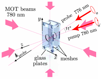
Figure 1: (Color online) Capacitor assembly and laser beam orientation. The MOT is formed close to the center of a flat capacitor consisting of two 80% transparent meshes glued to parallel glass plates with a mesh separation of 1 cm. The circularly $\sigma^{+}$ polarized pump beam at 780 nm is parallel to the electric field ($z$-axis) while the probe beam is directed at the angle of $11^{\circ}$ in the $z$-$y$ plane to the pump beam and is also circularly polarized (either $\sigma^{+}$ or $\sigma^{-}$) with respect to its wave vector $\bm{k}_{\textrm{probe}}$.

To measure the Stark shift of the 5D level in Rubidium we used two-stage laser excitation $5S\rightarrow 5P\rightarrow 5D$ in an external dc electric field on the order of 1 kV/cm. Rb-87 atoms were laser cooled in a regular six-beam magneto-optical trap (MOT) with an axial magnetic field gradient of up to 20 G/cm. The cloud of 300 $\mu$m in diameter contains about $10^{6}$ atoms at a temperature of 300 $\mu$K. The MOT configuration and the excitation scheme are similar to one described in Ref Snigirev . Compared to Ref. Snigirev , the atomic cloud was formed in the center of a plane capacitor consisting of two metallic meshes, as shown in Fig.1. The capacitor was placed inside a vacuum glass cell (3 cm$\times$3 cm$\times$12 cm) providing easy optical access.

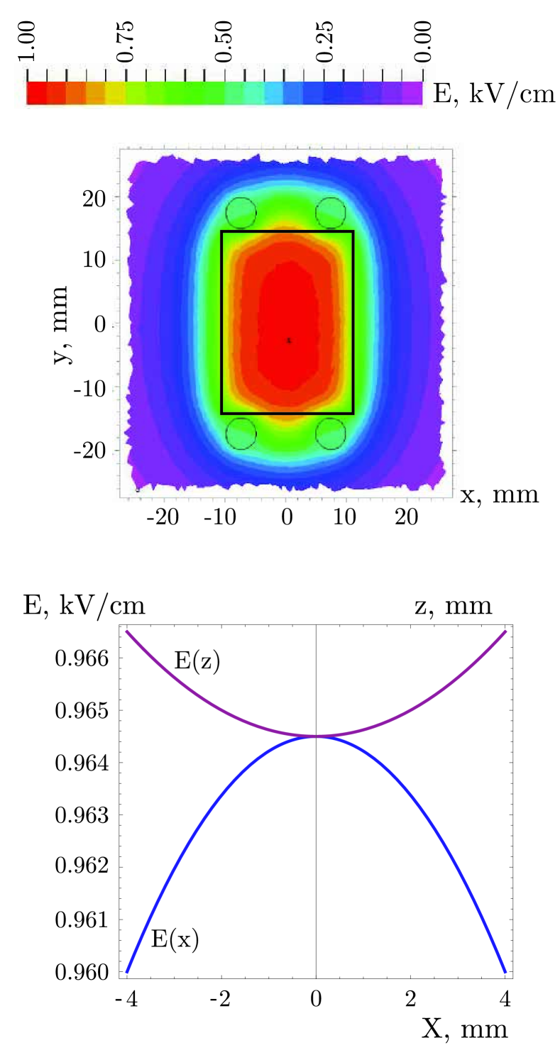
Figure 2: (Color online) Numerical calculations of the electric field distribution with 1 kV applied to the capacitor depicted in Fig.1. Top: field distribution at the central plane ($x$-$y$) of the capacitor.
Bottom: zoom in of the central volume. The origin is positioned at the geometric center of the capacitor.

The mesh consists of non-magnetic stainless steel wires with a diameter of 25 $\mu$m and has an optical transparency of 80%. To manufacture one of the capacitor plates the mesh was made taut and then glued to a flat glass plate with a hole of 1 cm in diameter. We saw to it that glue did not penetrate through the mesh to the front surface. Two plates were glued together using four glass posts of calibrated length, thus forming a plane capacitor with rectangular plates of $2\,\textrm{cm}\times 3$ cm and the separation of 1 cm. The distance between the plates and the hole size provides clearance for the laser cooling beams. One pair of laser cooling beams were sent through the mesh as shown in Fig.1, which did not significantly change the cloud shape or the number of atoms.

Although all glass components were manufactured in the Laboratory of Optics, P.N. Lebedev Physics Institute, and have superior flatness and well-defined sizes within a few $\mu$m, the glue can influence the distance $l$ between the meshes. To reach an uncertainty of 0.5% in polarizability one should know the electric field to 0.2%, which corresponds to 20 $\mu$m uncertainty in the distance.

The parallelism of the glass plates was checked in the air using a micrometer and found to be parallel to within $15^{\prime}$. This angle was taken into account in calculations of the electric field. The distance $l$ between the meshes was measured optically in vacuum using a high NA lens assembly ($F/D\approx 1$ ) which imaged a free standing mesh on a CCD camera. The lens and the camera were rigidly placed on a three-coordinate translation stage outside the vacuum chamber. The translation stage axis was aligned with $1^{\circ}$ accuracy perpendicular to the capacitor plate (along the $z$-axis, Fig. 1). The focus position for one of the meshes was determined from a number of shots using a gradient filter method and then by fitting the position of the translation stage to the highest image sharpness. This method provides a statistical uncertainty of 5 $\mu$m. Moving the translation stage in the $x$-$y$ direction we performed similar measurements in the region within $\pm$3 mm of the hole center. The distance remained constant within 20 $\mu$m, the scatter can be explained by the mesh thickness. The final result including the averaged mesh thickness gives $l=9.88(3)\,\textrm{mm}$. The refractive index of air contributes to the result on a negligible level.

The field distribution in our capacitor was simulated using a finite element analysis, the result for the $x$-$y$ plane as well as the zoom in of the central volume is shown in Fig.2(a). The position of the atomic cloud was controlled within $\pm 1$ mm with respect to the center of the capacitor by two CCD cameras. As follows from Fig. 2, the field variation within this volume is less than 0.05%. The potential difference between the plates could be varied from zero to 2.5 kV using a high-voltage power supply (Stanford Research Systems PS350). The accuracy of the device was studied with a high-precision voltmeter and corresponded to 0.1 % variation.

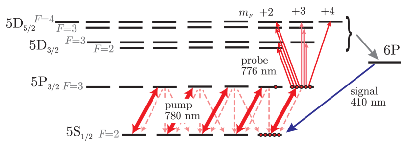
Figure 3: (Color online) Relevant energy levels in Rb-87 (not to scale) and excitation laser fields. Radiation at 780 nm coupling 5S_1/2 and 5P_3/2 levels was used for laser cooling and for optical pumping of Rb atoms. The pump beam was $\sigma^{+}$ polarized and directed along the $z$-axis (see Fig. 1), transferring population to the $5\textrm{P}_{3/2}(F=3,m_{F}=+3)$ level. The polarized probe laser beam at 776 nm was tuned in resonance to one of the hyperfine transitions $5\textrm{P}_{3/2}\rightarrow 5\textrm{D}_{3/2,\,5/2}$. Excitation of the 5D level was measured by spontaneous emission of 410 nm photons via the 6P level.

Measurement of the Stark shift of each of the $5\textrm{P}_{3/2}\rightarrow 5\textrm{D}_{3/2,\,5/2}$ transitions (Fig. 3) was performed in a pulsed regime, the pulse sequence was repeated every 20 $\mu$s and is depicted in Fig. 4. First, atoms were laser cooled using the 780 nm transition coupling $5\textrm{S}_{1/2}$ and $5\textrm{P}_{3/2}$ levels. Since the MOT is formed close to the zero of the quadrupole magnetic field, all magnetic sublevels of the $5\textrm{P}_{3/2}$ level become nearly equally populated, which does not allow for determination of polarizabilities (2), so we prepare the atoms into a particular magnetic state using optical pumping at 780 nm.

After switching off the MOT beams we waited for 200 ns and applied a circularly $\sigma^{+}$ polarized pump pulse along the $z$-axis (Fig. 1) to transfer atoms to the $5\textrm{P}_{3/2}(F=3,m_{F}=+3)$ magnetic state, as shown in Fig. 3. The pulse had an intensity of 100 mW/cm² and a duration of 500 ns, which is much longer than the reverse pumping rate. Experimental results presented in the next Section verify that nearly all atoms addressed by the probe 5P$\rightarrow$5D radiation were pumped into the $m_{F}=+3$ sublevel.

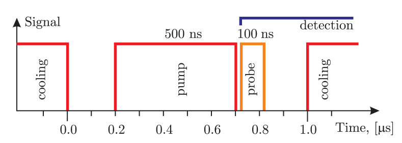
Figure 4: (Color online) Pulse sequence in our experiment. After laser cooling for 19 $\mu$s the cooling laser was switched off for 1 $\mu$s for optical pumping (780 nm, 500 ns) and probing the 5P$\rightarrow$5D transition (776 nm, 50 ns). To avoid the ac Stark shift from strong 780 nm pumping radiation while obtaining enough signal, the probe pulse was switched on 10 ns after the pump was switched off. Detection starts simultantously with the probe beam and lasts for $1\,\mu$s. The whole cycle was repeated every 20 $\mu$s, the MOT magnetic field was continuously on.

The probe beam at 776 nm was tuned close to resonance with one of the fine structure sublevels 5D_5/2, 3/2, which are separated by 89 GHz. The probe beam was directed at an angle of 11^∘ to the $z$-axis, allowing for independent control of its polarization. Polarization of the probe beam was changed from $\sigma^{+}$ to $\sigma^{-}$ with respect to its wave vector $\bm{k}_{\textrm{probe}}$. In this case we can address different magnetic sublevels of the 5D multiplet and thus derive polarizabilities using (2). Due to the set angle to the quantization axis, probe radiation always contains an admixture of linear polarized light (with respect to the $z$-axis), which is taken into account in our analysis. Thus, with the pump beam we couple the sublevel $5\textrm{P}_{3/2}(F=3,m_{F}=+3)$ either with one of the sublevels from $5\textrm{D}_{5/2}(F=3,\,4,\,m_{F}=+2,...,F)$ multiplet or with one from the $5\textrm{D}_{3/2}(F=2,\,3,\,m_{F}=+2,...,F),$ as shown in Fig. 3. The hyperfine structure of the 5D level is about 100 MHz and is well resolvable.

The probe pulse with an intensity of 100 mW/cm² was switched on right after the pump beam was switched off. The time delay between the two pulses was chosen to be 10 ns to avoid overlap between pulses. The strong pump beam causes an ac Stark shift of the 5P_3/2 level, which influences the results of our measurement. The 5P_3/2 level lifetime equals 30 ns and most of the atoms excited to the 5P_3/2 remain there when the probe beam is on. The probe pulse duration was 50 ns, which is much shorter than the 5D level lifetime (300 ns). This prevents optical pumping back to the 5P_3/2 level and re-distribution of the population between magnetic components.

Approximately 30% of atoms in the 5D state decay to the ground state via the 6P level, emitting 410 nm photons. In our experiment, ”blue” photons were collected onto a photomultiplier tube equipped with a narrow-band 410 nm filter. Photons were counted in a time window of 1 $\mu$s, as shown in Fig. 4. The probe laser was scanned over the resonance with an acousto-optical modulator (AOM). For each of the frequency steps (typically 50 per line) the signal was accumulated for 0.1 s. A typical count rate at the resonance position was $2\times 10^{4}$cps.

The MOT magnetic field gradient was continuously switched on. The influence of magnetic field on our results is discussed below.

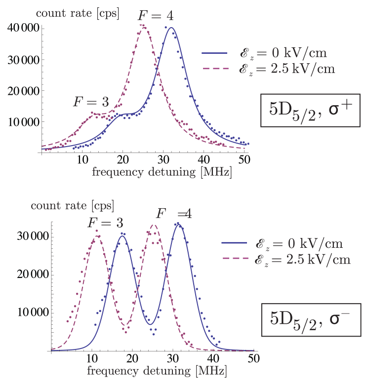
Figure 5: (Color online) Top: spectral line profiles of the $5\textrm{P}_{3/2}\rightarrow 5\textrm{D}_{5/2}$ transition with the probe beam $\sigma^{+}$ polarized along $\bm{k}_{\textrm{probe}}$. The dashed line corresponds to zero electric field, $\mathcal{E}=0$ kV/cm, and the solid line to $\mathcal{E}=2.5$ kV/cm. The hyperfine component $F=3$ is excited because the probe beam possesses a fraction of linear polarization if projected onto the $z$-axis. Bottom: the same experiment, but for the probe beam $\sigma^{-}$ polarized along its wave vector. The amplitude of $F=3$ significantly increases because the transition to the sublevel $5\textrm{D}(F=3,\,m_{F}=2)$ becomes allowed (see also Fig. 3). Fits are done by the model function (c) described in the text.

Measurement of the Stark shift for each of the lines $5\textrm{P}_{3/2}\rightarrow 5\textrm{D}_{3/2,\,5/2}$ was performed at different voltages on the capacitor plates. For each of the selected voltages three spectral lines were recorded, namely, with positive voltage polarity, grounded electrodes and negative polarity, to prevent any influence of charging. The zero-voltage data was also used in the data analysis.

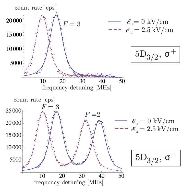
Figure 6: (Color online) Top: spectral line profiles of the $5\textrm{P}_{3/2}\rightarrow 5\textrm{D}_{3/2}$ transition with the probe beam $\sigma^{+}$ polarized with respect to $\bm{k}_{\textrm{probe}}$. The dashed line corresponds to zero electric field, $\mathcal{E}=0$ kV/cm, and the solid line to $\mathcal{E}=2.5$ kV/cm. The hyperfine component $F=3$ is clearly visible due to the component of linear polarization, but $F=2$ is not distinguishable from the noise. The spectrum proves the high efficiency of optical pumping and the absence of $\sigma^{-}$ component. Bottom: same experiment, but for the probe beam $\sigma^{-}$ polarized with respect to $\bm{k}_{\textrm{probe}}$. Now the component with $F=2$ is efficiently excited according to Fig. 3. Fits are done by the model function (c) described in the text.

IV Results and Data Analysis

Typical spectra of $5\textrm{P}_{3/2}\rightarrow 5\textrm{D}_{5/2}$ and $5\textrm{P}_{3/2}\rightarrow 5\textrm{D}_{3/2}$ transitions at different electric field strengths and probe beam polarizations are shown in Figs. 5, 6, respectively. From these spectra we derive the frequency shifts of the corresponding transitions, estimate the quality of initial state preparation and estimate the excitation probabilities to different magnetic sublevels of the 5D level.

The spectra were fitted by three different models: (a) sum of two Gaussian functions, (b) sum of two Lorentzian functions and (c) sum of two Lorentzian functions convoluted with the probe pulse spectral profile. The pulse shape was measured in Snigirev and its Fourier spectrum width equals 20 MHz for 50 ns duration. The model used 6 fit parameters: two amplitudes, two central frequencies and two widths. The different fit functions were used to test the model dependency of our fitting procedure and to evaluate the corresponding uncertainty. The fit gave us the frequency of each of the hyperfine components at different values of the electric field.

To derive the polarizability of the $5\textrm{D}_{5/2}$ level we used transitions from the $5\textrm{P}_{3/2}(F=3)$ level to two different hyperfine sublevels excited at different polarizations of the probe beam: $5\textrm{D}_{5/2}(F=4)$ (Fig. 5, top) and $5\textrm{D}_{5/2}(F=3)$ (Fig. 5, bottom). For the $5\textrm{D}_{3/2}$ level we use, respectively, $5\textrm{D}_{3/2}(F=3)$ (Fig. 6, top) and $5\textrm{D}_{3/2}(F=2)$ (Fig. 6, bottom). Since the probe beam radiation always contains a fraction of linearly polarized light if projected on the $z$-axis (tilted by 11^∘ with respect to $\bm{k}_{\textrm{probe}}$), all mentioned hyperfine components (except $5\textrm{D}_{3/2}(F=3)$) contain two different magnetic sublevels, as follows from Fig. 3. After projecting on the $z$-axis, the circularly polarized pump beam will consist of 96% circular polarization (the same sign) and 4% linear polarization.

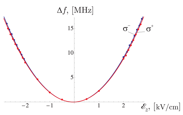
Figure 7: (Color online) Frequency shift of transitions to the $5\textrm{D}_{5/2}(F=4)$ and $5\textrm{D}_{5/2}(F=3)$ hyperfine sublelevs at different values of electric field $\mathcal{E}_{z}$. The polarization of the probe beam along $\bm{k}_{\textrm{probe}}$ was $\sigma^{+}$ and $\sigma^{-}$, respectively. A parabolic fit according to (5) is used.

Fig. 6 shows an example of the data for the $5\textrm{D}_{5/2}(F=4)$ and $5\textrm{D}_{5/2}(F=3)$ hyperfine sublelevs obtained at different electric field strengths. The difference in the two curves is due to the tensor polarizability. Fitting the data with parabolic dependence, $\Delta f=p\mathcal{E}^{2}$, according to (4,5) allows us to derive the sensitivity $p$ of each transition to the electric field. The results are:

$$p(5\textrm{D}_{5/2}(F=4),\,\sigma^{+}) = 2.014(8)\,\textrm{MHz}/(\textrm{kV/cm})^{2}\,,$$ (11)

$$p(5\textrm{D}_{5/2}(F=3),\,\sigma^{+}) = 2.087(8)\,\textrm{MHz}/(\textrm{kV/cm})^{2}\,,$$

$$p(5\textrm{D}_{3/2}(F=3),\,\sigma^{+}) = 2.066(8)\textrm{MHz}/(\textrm{kV/cm})^{2}\,,$$

$$p(5\textrm{D}_{3/2}(F=2),\,\sigma^{-}) = 2.158(9)\textrm{MHz}/(\textrm{kV/cm})^{2}\,,$$

where the entry in the parentheses after the level notation denotes the polarization of the probe beam.

The spectrum shown in Fig. 6 (top) contains only one hyperfine component, $5\textrm{D}_{3/2}(F=3)$. The $5\textrm{D}_{3/2}(F=2)$ one is not distinguishable from the noise. This component can be excited by the linearly polarized fraction of the probe beam from the $5\textrm{P}_{3/2}(F=3,\,m_{F}=+2)$ sublevel. Knowing the fraction of linear polarization in our probe beam, we can set a limit to the $5\textrm{P}_{3/2}(F=3,\,m_{F}=+2)$ sublevel population (see Table 2). Table 2 also shows the relative probabilities to excite different magnetic sublevels of the final $5\textrm{D}$ state, which are calculated using (5).

Table 2: The upper part of the table shows the quality of the optical pumping derived from Fig. 6 (top). The lower part presents relative probabilities to excite relevant hyperfine and magnetic sublevels of the $5\textrm{D}$ level at different polarizations of the probe beam.

initial state	$F,\,m_{F}$	population
$5\textrm{P}_{3/2}$	3, 3	$>0.97$
$5\textrm{P}_{3/2}$	3, 2	$<0.03$

final state	$F,\,m_{F}$	probe polarization	excitation
		(with respect to $\bm{k}_{\textrm{probe}}$)	probability
$5\textrm{D}_{5/2}$	4, 4	$\sigma^{+}$	0.64
$5\textrm{D}_{5/2}$	4, 3	$\sigma^{+}$	0.01
$5\textrm{D}_{5/2}$	3, 3	$\sigma^{-}$	0.004
$5\textrm{D}_{5/2}$	3, 2	$\sigma^{-}$	0.032
$5\textrm{D}_{3/2}$	3, 3	$\sigma^{+}$	0.024
$5\textrm{D}_{3/2}$	3, 2	$\sigma^{-}$	0.192
$5\textrm{D}_{3/2}$	2, 2	$\sigma^{-}$	0.192

Using the results (11), Table 2, and relation (5) we get a system of linear equations for different magnetic and hyperfine sublevels from which we derive scalar and tensor polarizabilities. Polarizabilities for the 5P level are taken from Windholz , their uncertainties negligibly contribute to our error budget.

Although the Rb cloud resides in the minimum of the MOT magnetic field, we expect a residual magnetic field on the order of 0.1 G due to the final cloud size and adjustment imperfections.

Switching off the magnetic field in the experiment takes about 500 $\mu$s, which would drastically reduce the duty cycle and the count rate. Therefore we decided to take the magnetic field into account instead of switching it off.

The influence of the magnetic field can be considered as additional degradation of the efficiency of the optical pumping. We found that magnetic field reduces relative population of the $5P_{3/2}(F=3,m=3)$ level in our experiment from 98% to 97%. More information about optical pumping in the magnetic field can be found in Appendix I.

To verify that the field does not significantly influence the results of our measurements, we measured the dependencies similar to that shown in Fig. 7 at axial magnetic field gradients of 10 G/cm and 5 G/cm. We did not observe any significant difference within the statistical uncertainty. Since our regular measurements were performed at a gradient of 10 G/cm, we conservatively add a systematic uncertainty to the $p$ values (11) of 0.1% due to the influence of the magnetic field.

The different fitting procedures (a,b,c) described above influence the results at the level of 0.03 %, so we add this value to the uncertainty of coefficients $p$ coming from the line shape model.

Calculation shows that the residual population of the 5P${}_{3/2}(F=3,\,m_{F}=2)$ level (see Table 2) can influence the coefficients $p$ on the level of 0.07%. Imperfection of the probe beam polarization and error in determination of the angle between the $z$-axis and $\bm{k}_{\textrm{probe}}$ also result in an uncertainty of 0.1 %.

Table 3: Uncertainty budget for coefficients $p$ describing the quadratic dependency on electric field (5), (11). Uncertainty of electric field determination is multiplied by 2 and included in this Table.

Effect	Uncertainty, %
Statistical uncertainty	0.2
Electric field determination	0.3
Residual magnetic field	0.1
Line shape model	0.03
Optical pumping	0.07
Probe beam polarization	0.1
AC Stark shift	0.1
Sum	0.41

The ac Stark shift of the 5P_3/2 level caused by a strong pump beam may influence the result of the measurement if the pump and probe pulses overlap. Experimental study of this effect shows that for the time delay used in the experiment (50 ns), the residual pump beam perturbs the result on the level of 0.1%.

All mentioned uncertainties, including the uncertainty of electric field determination, are summarized in Table 3. Adding up all contributing uncertainties quadratically, we get 0.4% for the coefficient $p$. This uncertainty directly converts in the uncertainty of scalar and tensor polarizability uncertainties as follows from (5). Since the main contribution to $p$ values comes from the scalar polarizability $\alpha_{S}$, its relative uncertainty is similar to the relative uncertainty of $p$. Tensor polarizability $\alpha_{T}$ is more than ten times smaller compared to $\alpha_{S}$, which means that its relative uncertainty is larger.

Scalar and tensor polarizabilities for the 5$D_{3/2,\,5/2}$ levels measured in our experiment and corresponding uncertainties are summarized in Table 4.

Table 4: Results for the tensor and scalar polarizability measurements of the 5$D_{3/2,\,5/2}$ levels in Rb-87 in atomic units. Here $\sigma$ is a standard deviation.

polarizability	value [atomic un.]	uncertainty, $\sigma$
$\alpha_{S}(5\textrm{D}_{3/2})$	18 400	75
$\alpha_{T}(5\textrm{D}_{3/2})$	$-$750	30
$\alpha_{S}(5\textrm{D}_{5/2})$	18 600	76
$\alpha_{T}(5\textrm{D}_{5/2})$	$-$1440	60

In conclusion, we determined the scalar and tensor polarizabilities of the 5D level in Rb. Using laser cooled atoms placed in a constant electric field and two-step laser excitation we demonstrated a relative uncertainty of 0.4% for the scalar polarizability and 4% for the tensor polarizability. The demonstrated uncertainty for the scalar polarizability is comparable to accurate measurements in ground state alkali atoms. Our result is close to the theoretical prediction Ovsiannikov where the model potential approach was implemented.

We are grateful to I. Veinstein and V. Ovsiannikov for discussions and acknowledge support from RFBR grants #12-02-00867-a and #11-02-00987-a.

V Appendix I: Optical pumping in the magnetic field

Consider an atom placed in the pumping beam propagating along the $z$ axis (Fig. 8). A magnetic field directed at some angle to the $z$ axis will cause precession of the magnetic moment of the atom and therefore changes in the populations of magnetic sublevels will occur. The maximum influence of the magnetic field will take place when it is perpendicular to the $z$ axis.

Changes in populations of magnetic sublevels due to optical pumping can be found by solving the master equation for the density matrix. Influence of the magnetic field can be calculated by projecting the initial wavefunction onto the basis with quantization axis along the direction of the magnetic field.

The initial wavefunction is $|\psi\rangle=\sum{c_{m}|m\rangle}$ where $|c_{m}|^{2}$ describes populations of the magnetic sublevels with projection of the magnetic moment onto the $z$ axis equal to $m$. In the new basis this wavefunction will have a form $|\psi\rangle=\sum{c_{m_{B}}|m_{B}\rangle}$ where $|m_{B}\rangle$ is a state with projection of the moment onto the direction of the magnetic field equal to $m_{B}$ and the coefficients $c_{m_{B}}$ can be calculated according to the equation:

$$c_{m_{B}}=\sum_{m}{c_{m}\int{Y^{F}_{m}(\theta,\phi)Y^{F}_{m_{B}}(\theta^{\prime},\phi^{\prime})^{*}\sin{\theta}d\theta d\phi}}.$$ (12)

Here the angles $\theta^{\prime}$ and $\phi^{\prime}$ can be expressed over $\theta$,$\phi$ and $\alpha$, where $\alpha$ is an angle between the original quantization axis and the magnetic field. If the magnetic field is perpendicular to the $z$ axis we have $\alpha=\pi/2$ and $\theta^{\prime}=\arccos(\sin\theta\,\cos\phi)$, $\phi^{\prime}=\arctan(\sin\phi\,\tan\theta)$. Taking into account evolution of the wavefunction in time we obtain:

$$|\psi\rangle=\sum{c_{m_{B}}|m_{B}\rangle e^{-i\frac{\mu_{B}g_{F}}{\hbar}m_{B}Bdt}},$$ (13)

where $g_{F}$ is the hyperfine Lande g-factor. Returning back to the initial basis, as in (12), we will obtain the new populations of the magnetic sublevels.

We accomplished numerical calculations of the population dynamics in the magnetic field perpendicular to the $z$ axis with 500 ns of optical pumping and further 100 ns evolution of the atom in the magnetic field without pumping. The results of the simulations for different values of the applied magnetic field are shown in Fig. 9. We can see that optical pumping remains efficient with magnetic fields up to 2 G. Larger fields leads to rapid mixing of states even during the pumping. Imperfection in the optical pumping in the experiment was about 3%, corresponding to a magnetic field less than 0.3 G.

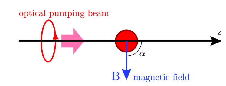
Figure 8: (Color online) An atom in a pumping beam and an external magnetic field. The pumping beam is propogating along the $z$ axis, which is selected as a quantization axis in the initial basis. Maximum influence of the magnetic field on the optical pumping process will take place when magnetic field is perpendicular to the $z$ axis.

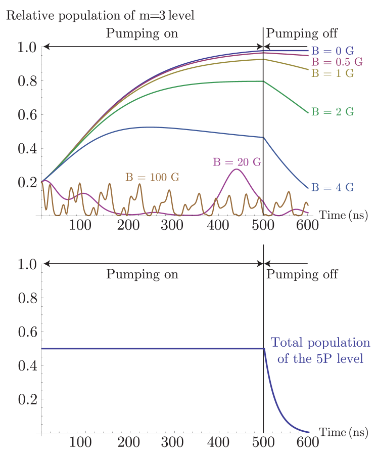
Figure 9: (Color online) Top: numerical calculations of the population of the magnetic level of $5P_{3/2}$ with $m=3$ during the optical pumping and after that. The population of the magnetic sublevel is normalized to the total population on the $5P_{3/2}$ level. Bottom: total population of the $5P_{3/2}$ level.

References

- (1) L. D. Landau and E.M. Lifshitz, Quantum Mechanics, Pergamon Press, New York, (1977).
- (2) J. Mitroy, M.S. Safronova, and Charles W. Clark, TOPICAL REVIEW: Theory and applications of atomic and ionic polarizabilities , J. Phys. B 43, 202001 (2010).
- (3) H. Katori, M. Takamoto, VG Pal’chikov, VD Ovsiannikov, Phys. Rev. Lett. 91, 173005 (2003).
- (4) K. Beloy, U.I. Safronova, A. Derevianko, Phys. Rev. Lett. 97, 040801 (2006).
- (5) Thomas Middelmann, Stephan Falke, Christian Lisdat, and Uwe Sterr, Phys. Rev. Lett. 109, 263004 (2012).
- (6) J.A. Sherman, N.D. Lemke,N. Hinkley, M. Pizzocaro, R.W. Fox, A.D. Ludlow, and C.W. Oates, Phys. Rev. Lett. 108, 153002 (2012).
- (7) S. Ulzega, A. Hofer, P. Moroshkin, A. Weis, Eur. Phys. Lett. 76, 1074 (2006).
- (8) A. Derevianko, W. R. Johnson, M. S. Safronova, and J. F. Babb, Phys. Rev. Lett. 82, 3589 (1999).
- (9) A. Miffre, M. Jacquey, M. Büchner, G. Trénec, and J. Vigué, Phys. Rev. A 73, 011603(R) (2006).
- (10) Jason M. Amini and Harvey Gould, Phys. Rev. Lett. 91, 153001 (2003).
- (11) William F. Holmgren, Raisa Trubko, Ivan Hromada, and Alexander D. Cronin, Phys. Rev. Lett. 109, 243004 (2012).
- (12) Axel Grabowski, Rolf Heidemann, Robert Löw, Jürgen Stuhler, and Tilman Pfau, Fortschritte der physik-progress of physic, 54 765-775 (2006).
- (13) M. S. Osullivan and B. P. Stoicheff, Phys. Rev. A 33 1640 (1986). 2003.
- (14) Jianming Zhao, Hao Zhang, Zhigang Feng, Xingbo Zhu, Linjie Zhang, Changyong Li, and Suotang Jia, Journal of the Physical Society of Japan 80 034303 (2011).
- (15) W. Hogervorst, and S. Svanberg, Physica Scripta. Vol. 12, 67, (1975).
- (16) D. Touahri, O. Acef, A. Clairon, J.-J. Zondy, R. Felder, L. Hilico, B. de Beauvoir, F. Biraben, and F. Nez, Opt. Commun. 133, pp. 471, (1997).
- (17) J. E. Bernard, A. A. Madej, K. J. Siemsen, L. Marmet, C. Latrasse, D. Touahri, M. Poulin, M. Allard, and M. Têtu, Opt. Commun. 173, 357, (2000).
- (18) T.J. Quinn, Practical realisation of the definition of the metre, including recommended radiations of other optical frequency standards (2001). Metrologia, 40:103 133,
- (19) N. L. Manakov, V. D. Ovsiannikov, J. Phys. B - atomic molecular and optical physics 10, 569 (1977).
- (20) A.A. Kamenski, V.D. Ovsiannikov, J. Phys. B. At. Mol. Opt. Phys. 39, 2247 (2006).
- (21) D.A. Kondrat’ev, I.L. Beigman, L.A. Vainshtein, Bulletin of the Lebedev Physics Institute 35, 12, 355 (2008).
- (22) L. A. Vainshtein, V. P. Shevelko, Program “Atom”, Preprint No. 43 of Lebedev Phys. Inst., Moscow, (1996).
- (23) V.D. Ovsiannikov, private communications.
- (24) Daniel A. Steck, “Rubidium 87 D Line Data,” available online at http://steck.us/alkalidata (revision 2.1.4, 23 December 2010).
- (25) C. Krenn, W. Scherf, O. Khait, M. Musso, and L. Windholz, Zeitschrift fur Physik D 41 , 229 (1997).
- (26) S.A. Snigirev, A.A. Golovizin, G.A. Vishnyakova, A.V. Akimov, V.N. Sorokin, N.N. Kolachevskii, Quantum Electron., 2012, 42 (8), 714 72