Compressed Sensing for Energy-Efficient Wireless Telemonitoring: Challenges and Opportunities

Abstract

As a lossy compression framework, compressed sensing has drawn much attention in wireless telemonitoring of biosignals due to its ability to reduce energy consumption and make possible the design of low-power devices. However, the non-sparseness of biosignals presents a major challenge to compressed sensing. This study proposes and evaluates a spatio-temporal sparse Bayesian learning algorithm, which has the desired ability to recover such non-sparse biosignals. It exploits both temporal correlation in each individual biosignal and inter-channel correlation among biosignals from different channels. The proposed algorithm was used for compressed sensing of multichannel electroencephalographic (EEG) signals for estimating vehicle drivers’ drowsiness. Results showed that the drowsiness estimation was almost unaffected even if raw EEG signals (containing various artifacts) were compressed by 90%.

I Introduction

Compressed sensing (CS) is a newly introduced data sampling and/or compression technology in wireless telemonitoring of biosignals . Compared to traditional data compression technologies, it consumes much less energy thereby extending sensor lifetime [1, 2, 3], making it attractive to wireless body-area networks [4].

The basic CS framework is an underdetermined inverse problem, which can be expressed as

$$\mathbf{y}=\mathbf{\Phi}\mathbf{x}+\mathbf{v},$$ (1)

where, in the context of data compression, $\mathbf{x}\in\mathbb{R}^{M\times 1}$ is a biosignal from a channel, $\mathbf{\Phi}\in\mathbb{R}^{N\times M}(N<M)$ is a user-designed measurement matrix, $\mathbf{v}\in\mathbb{R}^{N\times 1}$ is sensor noise, and $\mathbf{y}\in\mathbb{R}^{N\times 1}$ is the compressed signal. This compression task is performed in sensors of a wireless body-area network. Then the compressed signal $\mathbf{y}$, through Bluetooth, is sent to a nearby computer (and may be further sent to a remote computer via Internet). At the computer the original signal $\mathbf{x}$ is recovered by a CS algorithm using $\mathbf{y}$ and $\mathbf{\Phi}$. To successfully recover $\mathbf{x}$, $\mathbf{x}$ is required to be sparse. When $\mathbf{x}$ is not sparse, one generally seeks a dictionary matrix $\mathbf{D}$ such that $\mathbf{x}$ can be sparsely represented with the dictionary matrix, i.e., $\mathbf{x}=\mathbf{Dz}$, where the representation coefficients $\mathbf{z}$ are sparse. Generally, $\mathbf{D}$ is constructed using some bases, such as the bases of discrete Cosine transform (DCT) or Gabor basis. It can be also automatically learned from training data using dictionary learning. Then a CS algorithm can first recover $\mathbf{z}$ using the available $\mathbf{y}$ and $\mathbf{\Phi}\mathbf{D}$, and then recover $\mathbf{x}$ according to $\mathbf{x}=\mathbf{Dz}$. The basic CS framework has been widely used for biosignals [1, 5, 6, 3].

Noticing many biosignals have rich temporal correlation structures, recently Zhang et al. [7] suggested using block sparse Bayesian learning (BSBL) [8] to exploit such temporal correlation structures in order to achieve higher recovery performance. According to this model, the original signal $\mathbf{x}$ is assumed to have the following block structure:

$$\mathbf{x}=[\underbrace{x_{1},\cdots,x_{d_{1}}}_{\mathbf{x}_{1}^{T}},\cdots,\underbrace{x_{d_{g-1}+1},\cdots,x_{d_{g}}}_{\mathbf{x}_{g}^{T}}]^{T}$$ (2)

where $d_{i}(\forall i)$ are not necessarily identical. Entries in each block may be correlated and thus the correlation can be exploited to improve recovery performance [7]. The block structure can be also exploited to recover signals with less-sparse representation [9]. Extensive experiments showed that BSBL is a successful technique for compressed sensing of biosignals.

Another often-used CS model is the multiple measurement vector (MMV) model [10], which can be expressed as:

$$\mathbf{Y}=\mathbf{\Phi}\mathbf{X}+\mathbf{V},$$ (3)

where $\mathbf{X}\in\mathbb{R}^{M\times L}$ are multichannel biosignals (each column represents a biosignal from a channel), $\mathbf{Y}\in\mathbb{R}^{N\times L}$ are compressed signals, and $\mathbf{V}\in\mathbb{R}^{N\times L}$ is channel noise. Using this model, multichannel biosignals can be recovered simultaneously [6]. Theoretically, when columns of $\mathbf{X}$ are mutually independent, simultaneously recovering columns of $\mathbf{X}$ can achieve significantly higher recovery performance than treating (3) as $L$ independent problems and recovering each column of $\mathbf{X}$ separately. However, the benefit is compromised if columns of $\mathbf{X}$ are mutually correlated [11]. Thus the model brings limited performance improvement, since most multichannel biosignals have strong inter-channel correlation. Recently, we [11] showed that suitably exploiting the inter-channel correlation can greatly improve recovery performance.

In addition to the above models, there are many other models proposed to exploit various structure information of biosignals for better recovery performance, such as partially known support [12], and other expression methods of sparsity [13, 14]. Lots of efforts are also made to seek an optimal dictionary $\mathbf{D}$ such that biosignals have sparse representations [15, 16].

However, there is a challenge in compressed sensing of biosignals in wireless telemonitoring. The challenge is mainly due to non-sparseness of biosignals recorded during wireless telemonitoring. Thus most CS algorithms may not be suitable for use in wireless telemonitoring. Recently it is found that BSBL is a promising framework for recovering non-sparse signals [7] and signals with less sparse representations [9]. Motivated by this, in this work a novel spatio-temporal sparse Bayesian learning (STSBL) is proposed, which is an extension of BSBL. It jointly exploits temporal correlation in each biosignal and inter-channel correlation among biosignals from different channels to improve recovery performance. This study also evaluates the efficacy of the proposed algorithm on compressing multi-channel EEG data collected in a realistic driving task.

II The Challenge: Non-Sparsity

Many recorded biosignals in wireless telemonitoring are generally non-sparse in the time domain and in other transformed domains [7, 9]. Therefore, recovering these signals is a challenge to CS, since CS assumes signals are sparse in the time domain or in some transformed domain.

The non-sparsity mainly comes from various kinds of artifacts [17]. A main goal of wireless telemonitoring systems is wearable computing and ubiquitous monitoring of patients, where users can move freely. This unavoidably results in large artifacts in recorded signals. In addition, there are other artifacts resulting from electrode motion, unstable supply of batteries, baseline wander, and power-line interference.

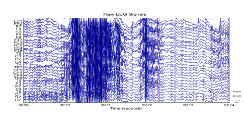
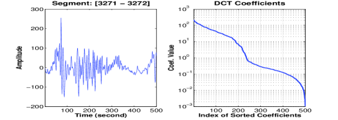
Fig.1 shows a segment of 30-channel EEG signals recorded by a wireless telemonitoring system when the subject was driving. Clearly, the signals were contaminated by very strong artifacts from muscle activity; they are non-sparse in the time domain and also non-sparse in the DCT domain (Fig.2). In particular, from Fig.2 we can see that the number of nonzero DCT coefficients of a segment is about $M/2$, where $M=500$ is the segment length. If compressing the EEG segment (of length $M$) into less than $M/2$ data points, using existing CS algorithms to recover the original EEG segment is extremely difficult or even impossible.

Figure 1: A segment of 30-channel raw EEG signals, in which strong artifacts appeared from the 3270 second and last for about 2 seconds. The signals were recorded with sampling frequency 250 Hz. The signals were recorded in our experiment.

Figure 2: The waveform (left) and the absolute values of DCT coefficients (right) of the EEG signal in Fig.1 from the 3271th to 3272th second at Channel FCz. Note that the number of significantly nonzero DCT coefficients is about 250, while the EEG segment length is 500. If compressing the EEG segment into less than 250 data points, using existing CS algorithms to recover the original EEG segment is extremely difficult or even impossible.

Figure 3: The relationship between sparsity (in the DCT domain) and sampling frequency. (a) is an ECG signal of 6 seconds. (b) shows the sorted absolute values of DCT coefficients of a segment (the first 2 seconds of the ECG signal) sampled at 360 Hz. (c) shows the sorted absolute values of DCT coefficients of the same segment but sampled at 120 Hz.

One may argue to remove these artifacts before data compression. However, this on-sensor processing can significantly raise hardware implementation cost and energy consumption of sensors. For example, to remove movement artifacts in EEG signals, independent component analysis (ICA) [18] is generally used. However, implementing an ICA algorithm in sensors increases hardware design complexity and energy consumption. It is more desired that no complicated processing is used when compressing a raw biosignal, while a CS algorithm can still recover it with high fidelity.

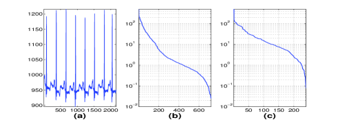
Non-sparsity can be also resulted from low sampling frequency. Fig.3 gives an example, where we can see when sampling frequency decreased, the DCT coefficients of an ECG signal become less sparse. This observation implies that recorded biosignals via wireless systems tend to be less sparse (in transformed domains), since sampling frequency for many biosignals (e.g. EEG and ECG) in wireless systems is typically about 150 – 250 Hz due to energy constraint in wireless systems.

III Spatio-Temporal Sparse Bayesian learning

III-A Motivation

The previous section shows the challenge for CS algorithms in recovering non-sparse biosignals or biosignals with non-sparse representation coefficients.

Exploiting structures in biosignals is a promising way to solving this challenge. For example, by exploiting block structures and intra-block correlation of raw abdominal signals recorded from a pregnant woman, we successfully reconstructed the signals using BSBL and extracted a clean fetal ECG by using ICA [7]. However, the BSBL algorithm is designed for recovering single-channel recordings. When recovering multichannel recordings, it has to recover the recordings channel by channel, which is time-consuming and thus not suitable for real-time telemonitoring of multichannel signals. Furthermore, the algorithm does not exploit inter-channel correlation among signals from different channels.

This section proposes a spatio-temporal sparse Bayesian learning (STSBL) algorithm. This algorithm not only exploits correlation structure in each channel as BSBL-BO, but also exploits inter-channel correlation among signals from different channels. Due to space constrains, the next section provides the main idea of the algorithm. Detailed algorithm derivation can be found in [19].

III-B Model

First, we give the following spatiotemporal compressed sensing model, which is the MMV model (3) but with more structures in each column of $\mathbf{X}$ :

$$\mathbf{Y}=\mathbf{\Phi}\mathbf{X}+\mathbf{V},$$ (4)

where $\mathbf{X}$ is assumed to have the following block structure:

$$\mathbf{X}=\left[\begin{array}[]{c}\mathbf{X}_{[1]\cdot}\\ \mathbf{X}_{[2]\cdot}\\ \vdots\\ \mathbf{X}_{[g]\cdot}\end{array}\right]$$ (9)

where $\mathbf{X}_{[i]\cdot}\in\mathbb{R}^{d_{i}\times L}$ is the $i$-th block of $\mathbf{X}$, and $\sum_{i=1}^{g}d_{i}=M$. The key assumption is that each block $\mathbf{X}_{[i]\cdot}(\forall i)$ is assumed to have spatiotemporal correlation. In other words, entries in each column of $\mathbf{X}_{[i]\cdot}$ are correlated (i.e., each signal is temporally correlated), and entries in each row of $\mathbf{X}_{[i]\cdot}$ are also correlated (i.e., signals from different channels are spatially correlated).

To facilitate algorithm development, we make the same assumptions as in the standard multivariate Bayesian variable selection model (also called the conjugate multivariate linear regression model) [20]. The $i$-th block $\mathbf{X}_{[i]\cdot}$ is assumed to have the parameterized Gaussian distribution $p(\mathrm{vec}(\mathbf{X}_{[i]\cdot}^{T});\gamma_{i},\mathbf{B},\mathbf{A}_{i})=\mathcal{N}(\mathbf{0},(\gamma_{i}\mathbf{A}_{i})\otimes\mathbf{B})$. Here $\mathbf{B}\in\mathbb{R}^{L\times L}$ is an unknown positive definite matrix capturing the correlation structure in each row of $\mathbf{X}_{[i]\cdot}$. The matrix $\mathbf{A}_{i}\in\mathbb{R}^{d_{i}\times d_{i}}$ is an unknown positive definite matrix capturing the correlation structure in each column of $\mathbf{X}_{[i]\cdot}$. $\gamma_{i}$ is an unknown nonnegative scalar determining whether the $i$-th block is a zero block or not, and its positive value also determines the norm of the $i$-th block. Assuming the blocks $\{\mathbf{X}_{[i]\cdot}\}_{i=1}^{g}$ are mutually independent, the distribution of the matrix $\mathbf{X}$ is

$$p(\mathrm{vec}(\mathbf{X}^{T});\mathbf{B},\{\gamma_{i},\mathbf{A}_{i}\}_{i})=\mathcal{N}(\mathbf{0},\mathbf{\Pi}\otimes\mathbf{B})$$ (10)

where $\mathbf{\Pi}$ is a block diagonal matrix with the $i$-th principal diagonal block given by $\gamma_{i}\mathbf{A}_{i}$. Besides, each row of the noise matrix $\mathbf{V}$ is assumed to have the distribution $p(\mathbf{V}_{i\cdot};\lambda,\mathbf{B})=\mathcal{N}(\mathbf{0},\lambda\mathbf{B})$, where $\lambda$ is an unknown scalar. Assuming the rows are mutually independent, we have

$$p(\mathrm{vec}(\mathbf{V}^{T});\lambda,\mathbf{B})=\mathcal{N}(\mathbf{0},\lambda\mathbf{I}\otimes\mathbf{B}).$$ (11)

In our model $\mathbf{X}$ and $\mathbf{V}$ share the common matrix $\mathbf{B}$ for modeling the spatial correlation. This is a traditional setting in Bayesian variable selection models [20]. Besides, since in our application sensor noise $\mathbf{V}$ can be ignored , the covariance model of $\mathbf{V}$ is not important. It only facilitates the development of our algorithm.

Due to the coupling between $\mathbf{A}_{i}(\forall i)$ and $\mathbf{B}$, directly estimating parameters in the model (4) can result in an algorithm with heavy computational load. However, we observe that the original model can be transformed into two equivalent models, where we can efficiently estimate parameters by alternating between the two models. This largely simplifies the algorithm development.

III-C Learning in the Model with $\mathbf{B}$ Given

Assume $\mathbf{B}$ is known. Letting $\widetilde{\mathbf{Y}}\triangleq\mathbf{Y}\mathbf{B}^{-\frac{1}{2}}$, $\widetilde{\mathbf{X}}\triangleq\mathbf{X}\mathbf{B}^{-\frac{1}{2}}$, and $\widetilde{\mathbf{V}}\triangleq\mathbf{V}\mathbf{B}^{-\frac{1}{2}}$, the original model (4) becomes

$$\widetilde{\mathbf{Y}}=\mathbf{\Phi}\widetilde{\mathbf{X}}+\widetilde{\mathbf{V}},$$ (12)

where the spatial correlation in $\widetilde{\mathbf{X}}$ and $\widetilde{\mathbf{V}}$ is removed. Clearly, the model (12) is a simple extension of the block sparse model with intra-block correlation [8] to the case of multiple measurement vectors. Therefore, following the EM estimation method in [8], we can easily estimate the parameters $\mathbf{X},\lambda,\{\gamma_{i},\mathbf{A}_{i}\}$. Details can be found in [19].

In this model we have assumed that $\mathbf{B}$ is given. This parameter can be estimated in the following equivalent model when assuming $\mathbf{X},\lambda,\{\gamma_{i},\mathbf{A}_{i}\}$ are given.

III-D Learning in the Model with $\mathbf{A}_{i}$ Given

To estimate the matrix $\mathbf{B}$, we consider the following equivalent form of the original model (4):

$$\mathbf{Y}=\overline{\mathbf{\Phi}}\cdot\overline{\mathbf{X}}+\mathbf{V}$$ (13)

where $\overline{\mathbf{\Phi}}\triangleq\mathbf{\Phi}\mathbf{A}^{\frac{1}{2}}$, $\overline{\mathbf{X}}\triangleq\mathbf{A}^{-\frac{1}{2}}\mathbf{X}$, and $\mathbf{A}$ is defined as $\mathbf{A}\triangleq\mathrm{diag}\{\mathbf{A}_{1},\cdots,\mathbf{A}_{g}\}$. In this model, $\overline{\mathbf{X}}$ maintains the same block structure as $\mathbf{X}$, but the temporal correlation of each signal is removed. Clearly, the model (13) is the same as the MMV model in [11] except that each column of $\overline{\mathbf{X}}$ has block partition. Following the approach in [11] we can derive the updating rule for $\mathbf{B}$.

III-E Combined Algorithm

Above we have derived the updating rules for $\mathbf{X}$, $\{\mathbf{A}_{i}\}_{i}$, $\{\gamma_{i}\}_{i}$ and $\lambda$ in the model given $\mathbf{B}$ and the updating rule for $\mathbf{B}$ in the model given $\{\mathbf{A}_{i}\}$. Combining these updating rules we obtain the EM-based spatiotemporal SBL algorithm, denoted by STSBL-EM. Table 1 summarizes the STSBL-EM algorithm when used in wireless telemonitoring, where sensor noise $\mathbf{V}$ is ignored (artifacts in biosignals are incorporated into $\mathbf{X}$). In this noise-free situation, the parameter $\lambda$ can be simply set to a very small value, such as $\lambda=10^{-10}$.

Algorithm 1 STSBL-EM For Noiseless Scenarios

  Input: $\mathbf{Y}$, $\mathbf{\Phi}$, and the block partition $\{d_{1},\cdots,d_{g}\}$.

  Output: $\mathbf{X}$

  Initialization: $\mathbf{X}$ is assigned by the Least Square solution; $\mathbf{A}_{i}=\mathbf{I}_{d_{i}}(\forall i)$; $\gamma_{i}=1(\forall i)$; $\lambda=10^{-10}$

  while not satisfy convergence criterion do

     $\check{\mathbf{B}}\leftarrow\sum_{i=1}^{g}\gamma_{i}^{-1}\mathbf{X}_{[i]\cdot}^{T}\mathbf{A}_{i}^{-1}\mathbf{X}_{[i]\cdot}$

     $\mathbf{B}\leftarrow\check{\mathbf{B}}/\|\check{\mathbf{B}}\|_{\mathcal{F}}$

     $\boldsymbol{\mu}\leftarrow\mathbf{\Pi}\mathbf{\Phi}^{T}(\lambda\mathbf{I}+\mathbf{\Phi}\mathbf{\Pi}\mathbf{\Phi}^{T})^{-1}\mathbf{Y}\mathbf{B}^{-\frac{1}{2}}$

     $\mathbf{\Sigma}\leftarrow\mathbf{\Pi}-\mathbf{\Pi}\mathbf{\Phi}^{T}(\lambda\mathbf{I}+\mathbf{\Phi}\mathbf{\Pi}\mathbf{\Phi}^{T})^{-1}\mathbf{\Phi}\mathbf{\Pi}$

     $\gamma_{i}\leftarrow\frac{1}{Ld_{i}}\sum_{l=1}^{L}\mathrm{Tr}\Big{[}\mathbf{A}_{i}^{-1}\big{(}\mathbf{\Sigma}_{[i]}+\boldsymbol{\mu}_{[i]l}\boldsymbol{\mu}_{[i]l}^{T}\big{)}\Big{]}$, ($\forall i$)

     $\mathbf{A}_{i}\leftarrow\frac{1}{L}\sum_{l=1}^{L}\frac{\mathbf{\Sigma}_{[i]}+\boldsymbol{\mu}_{[i]l}\boldsymbol{\mu}_{[i]l}^{T}}{\gamma_{i}}$, ($\forall i$)

     $\mathbf{X}\leftarrow\boldsymbol{\mu}\mathbf{B}^{\frac{1}{2}}$

  end while

IV Application

EEG-based drivers’ drowsiness monitoring is an emerging technology for driving safety [21, 22, 23]. The monitoring systems are powered by batteries and are generally embedded in a regular hat worn by drivers. Thus it is highly desired to develop EEG systems with low energy consumption [22]. The following subsections evaluate the proposed method with the multichannel EEG collected in a simulated driving task.

IV-A Experiment Settings

The EEG data were recorded with sampling rate 250 Hz from a subject using a 30-channel EEG system, when the subject was driving with drowsiness in a realistic kinesthetic virtual-reality car. Details on the recording system, the recording procedure, and the virtual-reality driving simulator, and the data are given in [22]. The driving task required the subject to maintain his cruising position and compensate for randomly induced lane deviations using the steering wheel. The deviation between the center of the vehicle and the center of the cruising lane was treated as the driving error. It is shown that the driving error is a good indicator to drowsiness level [22, 23].

Many methods were proposed to estimate the drowsiness level from recorded EEG signals. One method is first performing on-line ICA decomposition [18] on the signals, and then selecting an independent component (IC) to estimate its time-varying log power spectrum density (PSD), which is treated as an estimate of the drowsiness level. Details on this method can be found in [23].

The goal in this experiment was to show that the proposed algorithm can largely compress raw EEG signals (see Fig.1 for an example) before transmission and recover the signals in a remote computer (or a car-based computer) with high fidelity. For this goal, the raw 30-channel EEG signals of every 2 seconds were first compressed according to $\mathbf{Y}=\mathbf{\Phi}\mathbf{X}$, where $\mathbf{X}$ was the raw 30-channel EEG signals of 2 seconds, $\mathbf{\Phi}$ was a sparse binary matrix of the size $45\times 500$ (i.e. EEG was compressed by 90%) and each column of $\mathbf{\Phi}$ contains only two nonzero entries with value 1. The compressed data $\mathbf{Y}$ were sent to a nearby computer via blue-tooth, where the proposed STSBL-EM algorithm was performed to recover the original raw signals. Then the drowsiness was estimated using the recovered signals by the method in [23].

To examine whether the drowsiness estimate is degraded when using the recovered signals, we compared the drowsiness estimate using the recovered signals to the drowsiness estimate using the original signals. The procedure is as follows:

1. Apply the drowsiness estimation method in [23] on the original signals by performing ICA decomposition and selecting an IC (denoted by $\mathrm{IC}_{0}$) and a frequency $f$.

2. Apply the same drowsiness estimation method on the recovered signals by performing the same ICA decomposition and selecting an IC with the highest Pearson correlation with $\mathrm{IC}_{0}$ and selecting the same frequency $f$.

3. Evaluate the Pearson correlation between the drowsiness estimate in Step 1) and the drowsiness estimate in Step 2).

In our experiment, $\mathrm{IC}_{0}$ was an IC whose log PSD at the theta band (4-7 Hz) had high correlation with the driving error, and $f$ was 5 Hz.

For performance comparison, we performed other CS algorithms. They were BSBL-BO [8], Simultaneous OMP (SOMP) [24], and temporal M-FOCUSS (tMFOCUSS) [25]. BSBL-BO is a powerful algorithm with ability to recover less-sparse and non-sparse physiological signals [7, 9]. In [7] ten state-of-the-art CS algorithms including those exploiting block structures were shown to be inferior to BSBL-BO. SOMP and tMFOCUSS are two CS algorithms for jointly recovering multichannel signals. SOMP has been used in [6] to jointly recover multichannel EEG signals. When using STSBL-EM and BSBL-BO, the maximum iteration number was set to 40, and the block partition of both algorithms was set to ${d_{1}=d_{2}=\cdots=25}$. As in most literature [9, 6], all the algorithms recovered signals in a transformed domain, and the dictionary matrix $\mathbf{D}$ was a DCT dictionary matrix . Particularly, BSBL-BO recovered representation coefficient vectors in the transformed domain one by one, while STSBL-EM, tMFOCUSS, and SOMP jointly recovered the representation coefficient vectors.

Experiments were carried out on a computer with dual-core 2.9 GHz CPU and 6.0 GiB RAM.

Figure 4: Comparison of (a) the driving error (i.e. the drowsiness index), (b) the estimated drowsiness from the original EEG signals, and (c) the estimated drowsiness from the reconstructed EEG signals by STSBL-EM. The EEG recordings were compressed by 90%. The Pearson correlation between (b) and (c) was 0.96, showing the estimated drowsiness from reconstructed EEG signals by STSBL-EM was very close to the ground-truth (i.e. the estimated drowsiness from the original EEG signals).

Figure 5: Estimated drowsiness from the EEG signals recovered by (a) tMFOCUSS, (b) SOMP, and (c) BSBL-BO. The EEG signals were compressed by 90%. The Pearson correlation of (a) and the ground-truth (Fig.4(b)) was 0.91. The Pearson correlation of (b) and the ground-truth was 0.87. The Pearson correlation of (c) and the ground-truth was 0.85. The red circles highlight obviously distorted estimates.

IV-B Experimental Results

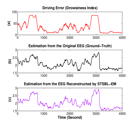
Fig.4 shows the recorded driving error (served as the drowsiness index), the drowsiness estimate using the original EEG signals, and the drowsiness estimate using the recovered EEG signals by STSBL-EM (note that the EEG signals were compressed by 90% before transmission). Clearly, the drowsiness estimate using the recovered signals was almost the same as the drowsiness estimate using the original signals.

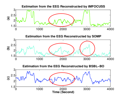
Fig.5 shows the drowsiness estimates using the recovered signals by tMFOCUSS, SOMP, and BSBL-BO. The estimates were obviously degraded. Particularly, some fluctuations of drowsiness (as indicated by the red circles in Fig.5), which are important for drowsiness detection and safety control, were seriously distorted.

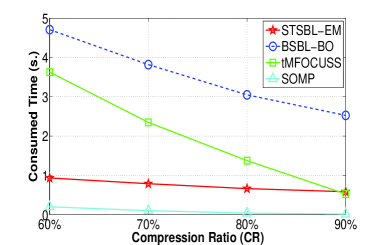
Fig. 6 shows the averaged consumed time of all algorithms in recovery of the 30-channel EEG signals of 2 seconds duration at different compression ratios. The compression ratio is defined as $CR=\frac{M-N}{M}\times 100\%$ with $M$ fixed to 500. The results show that STSBL-EM is very faster than BSBL-BO and thus is more suitable for practical use.

Figure 6: Averaged consumed time of all algorithms in recovery of the 30-channel signals of 2 seconds duration at different compression ratios. BSBL-BO has slow speed because it had to recover these signals channel by channel.

V Conclusions

This work proposed a spatiotemporal sparse Bayesian learning algorithm for energy-efficient compressed sensing of multichannel biosignals in wireless telemonitoring. In contrast to current compressed sensing algorithms, it not only exploits temporal correlation within each biosignal, but also exploits spatial correlation among biosignals from different channels. Compared to state-of-the-art algorithms, it has the best recovery performance and high speed. An experiment on EEG-based drivers’ drowsiness estimation showed that the proposed algorithm can ensure the drowsiness estimate on recovered EEG signals is almost the same as the estimate on original signals, even when the signals are compressed by 90%.

References

- [1] H. Mamaghanian, N. Khaled, D. Atienza, and P. Vandergheynst, “Compressed sensing for real-time energy-efficient ECG compression on wireless body sensor nodes,” IEEE Trans. Biomed. Eng., vol. 58, pp. 2456–2466, 2011.
- [2] B. Liu, Z. Zhang, G. Xu, H. Fan, and Q. Fu, “Energy efficient telemonitoring of physiological signals via compressed sensing: A fast algorithm and power consumption evaluation,” arXiv preprint arXiv:1309.7843, 2013.
- [3] F. Chen, A. Chandrakasan, and V. Stojanovic, “Design and analysis of a hardware-efficient compressed sensing architecture for data compression in wireless sensors,” IEEE Journal of Solid-State Circuits, vol. 47, no. 3, pp. 744–756, 2012.
- [4] A. Milenkovic, C. Otto, and E. Jovanov, “Wireless sensor networks for personal health monitoring: Issues and an implementation,” Computer communications, vol. 29, no. 13-14, pp. 2521–2533, 2006.
- [5] A. M. Dixon, E. G. Allstot, D. Gangopadhyay, and D. J. Allstot, “Compressed sensing system considerations for ECG and EMG wireless biosensors,” IEEE Trans. Biomed. Circuits Syst., vol. 6, no. 2, pp. 156–166, 2012.
- [6] S. Aviyente, “Compressed sensing framework for EEG compression,” in IEEE/SP 14th Workshop on Statistical Signal Processing, 2007, pp. 181–184.
- [7] Z. Zhang, T.-P. Jung, S. Makeig, and B. D. Rao, “Compressed sensing for energy-efficient wireless telemonitoring of noninvasive fetal ECG via block sparse Bayesian learning,” IEEE Trans. Biomed. Eng., vol. 60, no. 2, pp. 300–309, 2013.
- [8] Z. Zhang and B. D. Rao, “Extension of SBL algorithms for the recovery of block sparse signals with intra-block correlation,” IEEE Trans. on Signal Processing, vol. 61, no. 8, pp. 2009–2015, 2013.
- [9] Z. Zhang, T.-P. Jung, S. Makeig, and B. D. Rao, “Compressed sensing of EEG for wireless telemonitoring with low energy consumption and inexpensive hardware,” IEEE Trans. on Biomedical Engineering, vol. 60, no. 1, pp. 221–224, 2013.
- [10] S. F. Cotter, B. D. Rao, K. Engan, and K. Kreutz-Delgado, “Sparse solutions to linear inverse problems with multiple measurement vectors,” IEEE Trans. on Signal Processing, vol. 53, no. 7, pp. 2477–2488, 2005.
- [11] Z. Zhang and B. D. Rao, “Sparse signal recovery with temporally correlated source vectors using sparse Bayesian learning,” IEEE Journal of Selected Topics in Signal Processing, vol. 5, no. 5, pp. 912–926, 2011.
- [12] L. F. Polania, R. E. Carrillo, M. Blanco-Velasco, and K. E. Barner, “Compressed sensing based method for ecg compression,” in 2011 IEEE International Conference on Acoustics, Speech and Signal Processing (ICASSP), pp. 761–764.
- [13] J. K. Pant and S. Krishnan, “Compressive sensing of electrocardiogram signals by promoting sparsity on the second-order difference and by using dictionary learning,” IEEE Trans. Biomed. Circuits Syst., 2013.
- [14] Y. Liu, M. De Vos, I. Gligorijevic, V. Matic, Y. Li, and S. Van Huffel, “Multi-structural signal recovery for biomedical compressive sensing,” IEEE Trans. Biomed. Eng., vol. 60, no. 10, pp. 2794 – 2805, 2013.
- [15] A. M. Abdulghani, A. J. Casson, and E. Rodriguez-Villegas, “Compressive sensing scalp EEG signals: implementations and practical performance,” Medical and Biological Engineering and Computing, vol. 50, no. 11, pp. 1137–1145, 2012.
- [16] M. Mohsina and A. Majumdar, “Gabor based analysis prior formulation for EEG signal reconstruction,” Biomedical Signal Processing and Control, vol. 8, pp. 951–955, 2013.
- [17] T. Martin, E. Jovanov, and D. Raskovic, “Issues in wearable computing for medical monitoring applications: a case study of a wearable ECG monitoring device,” in The Fourth International Symposium on Wearable Computers, 2000.
- [18] T.-W. Lee, M. Girolami, and T. J. Sejnowski, “Independent component analysis using an extended infomax algorithm for mixed subgaussian and supergaussian sources,” Neural computation, vol. 11, no. 2, pp. 417–441, 1999.
- [19] Z. Zhang, T.-P. Jung, S. Makeig, Z. Pi, and B. D. Rao, “Spatiotemporal sparse Bayesian learning with applications to compressed sensing of multichannel physiological signals,” IEEE Trans. on Neural Systems and Rehabilitation Engineering, 2014.
- [20] P. Brown, M. Vannucci, and T. Fearn, “Multivariate bayesian variable selection and prediction,” Journal of the Royal Statistical Society: Series B (Statistical Methodology), vol. 60, no. 3, pp. 627–641, 1998.
- [21] T.-P. Jung, S. Makeig, M. Stensmo, and T. J. Sejnowski, “Estimating alertness from the eeg power spectrum,” IEEE Trans. Biomed. Eng., vol. 44, no. 1, pp. 60–69, 1997.
- [22] C. Lin, L. Ko, J. Chiou et al., “Noninvasive neural prostheses using mobile and wireless EEG,” Proceedings of the IEEE, vol. 96, no. 7, pp. 1167–1183, 2008.
- [23] C.-T. Lin, R.-C. Wu, S.-F. Liang et al., “Eeg-based drowsiness estimation for safety driving using independent component analysis,” Circuits and Systems I: Regular Papers, IEEE Trans. on, vol. 52, no. 12, pp. 2726–2738, 2005.
- [24] M. F. Duarte, S. Sarvotham, D. Baron, M. B. Wakin, and R. G. Baraniuk, “Distributed compressed sensing of jointly sparse signals,” in Asilomar Conf. Signals, Sys., Comput., 2005.
- [25] Z. Zhang and B. D. Rao, “Iterative reweighted algorithms for sparse signal recovery with temporally correlated source vectors,” in 2011 IEEE International Conference oncAcoustics, Speech and Signal Processing (ICASSP), pp. 3932–3935.