Improving the performance of algorithms to find communities in networks
Abstract
Most algorithms to detect communities in networks typically work without any information on the cluster structure to be found, as one has no a priori knowledge of it, in general. Not surprisingly, knowing some features of the unknown partition could help its identification, yielding an improvement of the performance of the method. Here we show that, if the number of clusters were known beforehand, standard methods, like modularity optimization, would considerably gain in accuracy, mitigating the severe resolution bias that undermines the reliability of the results of the original unconstrained version. The number of clusters can be inferred from the spectra of the recently introduced non-backtracking and flow matrices, even in benchmark graphs with realistic community structure. The limit of such two-step procedure is the overhead of the computation of the spectra.
pacs:
89.75.HcI Introduction
Community structure is one of the most important features of complex networks. Communities, or clusters, are subgraphs of a network with an unusually high density of edges, with respect to the average edge density of the network as a whole. Nodes in the same community tend to share the same attributes and/or roles within the network, and their identification might lead to the discovery of unknown features purely from topological inputs. This is why the quest for methods to detect communities in networks has become one of the hottest topics in network science Girvan and Newman (2002); Fortunato (2010).
In general, the only preliminary information available to any algorithm is the topology of the network, i.e. which pairs of nodes are connected to each other and which are not. Anything about the cluster structure to be found is unknown and is supposed to be given as output of the procedure. It would be valuable to have some information on the unknown partition of the network, as one could reduce considerably the huge space of possible partitions to explore, and increase the chance of successfully identifying the communities. In particular, if the number of clusters were known and could be given as input/constraint, methods deliver more accurate partitions.
The problem is that it is difficult to have access to the number of clusters. Fortunately, recent work has shown that it is possible to derive this information from the spectra of the non-backtracking matrix Krzakala et al. (2013) and the flow matrix Newman (2013), at least on the classic version of the planted partition model Condon and Karp (2001), where clusters have identical size and nodes the same degree (on average). We show that the prediction of the number of clusters remains accurate as well on the LFR benchmark graph Lancichinetti et al. (2008), which extends the original planted partition model by introducing realistic features of community structure, i.e. heterogeneous distributions of degrees and cluster sizes. The prediction is more reliable the larger the graph size.
Therefore, we propose to improve the performance of community detection algorithms via a two-step approach: first one infers the number of clusters from the spectrum of the non-backtracking or the flow matrix; then one uses this number as additional input of the algorithm. We show that popular methods, like the optimization of the modularity by Newman and Girvan Newman (2004), become much more accurate this way. This is remarkable, as the direct optimization of modularity is known to have a limited resolution, which may prevent the method from identifying the correct scale of the communities, even when the latter are very pronounced Fortunato and Barthélemy (2007); Good et al. (2010). Knowing the number of clusters , and constraining the optimization of the measure among partitions with fixed , one can mitigate the problem.
The computation of the spectra is unfortunately quite heavy, and represents the bottleneck of the procedure, making the analysis of large networks ( links) basically unfeasible. However, our results are encouraging and might stimulate the development of quicker approximate heuristics than the ones currently available.
In Section II we reveal the importance of knowing the number of clusters for the results of popular algorithms. Section III tests the reliability of the prediction of the number of clusters in the standard planted partition model and in the LFR benchmark graph. In Section IV we introduce a two-step approach consisting of a fast greedy optimization of the modularity by Newman and Girvan for partitions with a fixed number of clusters and we show the superiority of its performance with respect to the exhaustive modularity optimization via simulated annealing on the LFR benchmark. Our findings are summarized in Section V.
II Constrained versus unconstrained community detection
Stochastic block-models are the best known and most exploited class of models of networks with community structure. A graph with nodes is divided into groups of equal size , and the probability of nodes and to be linked is given by , where and are the groups of and , respectively. The principle is that the linking probability of any two nodes only depends on the memberships of the nodes. Despite its simplicity, this model can generate a wide variety of scenarios. Here we shall focus on the simplest one, where and . Here, if , the expected number of neighbors of a node within its group exceeds the expected number of neighbors of the node in each of the remaining groups, so the groups are communities according to the general intuition. This version coincides with the planted partition model by Condon and Karp Condon and Karp (2001), and has generated popular benchmark graphs that are regularly used to test the performance of community detection techniques, like the four-groups test Girvan and Newman (2002) and the LFR benchmark Lancichinetti et al. (2008).
According to the model, clusters are present and should be detectable so long as . However, recent works Reichardt and Leone (2008); Decelle et al. (2011a, b); Nadakuditi and Newman (2012); Floretta et al. (2013) have pointed out that, in the limit of sparse graphs, i.e. of networks of infinite size but finite average degree, random fluctuations make the detectability of clusters possible only for , where is a function of the parameters . So it is necessary for the clusters to have an internal edge density higher by some finite amount than the external one(s) to overcome the noise coming from the inherent stochasticity of the network’s construction. By introducing the average internal and external degree of a node in a cluster, and , respectively, the formula of the detectability limit derived in Refs. Decelle et al. (2011a); Nadakuditi and Newman (2012) reads
| (1) |
Typically, one fixes the value of the internal average degree and obtains the limit value of from Eq. 1, beyond which no method can do better than a random guess, which yields , where is the number of clusters.
In Fig. 1 we show the performance of several popular community detection algorithms on such model, in the simple case of two clusters (). Each panel corresponds to a different value of the cluster size , ranging from to . The average internal degree is fixed to . Given these parameters, Eq. 1 yields a value for the detectability limit (dashed vertical line), regardless of the cluster size , and we vary from to . The dot-dashed line indicates the limit performance of spectral modularity optimization, analytically derived in Ref. Nadakuditi and Newman (2012). Performance is computed as the fraction of correctly detected nodes Nadakuditi and Newman (2012). If all nodes are correctly assigned to their planted clusters, the fraction of correctly detected nodes is . As long as clusters are detectable, it stays above the value corresponding to random assignment (here , marked by the horizontal dashed line). The algorithms we adopted are: modularity optimization via simulated annealing (Mod) Guimerà et al. (2004), the Absolute Potts Model (APS) Ronhovde and Nussinov (2010), OSLOM Lancichinetti et al. (2011) and Infomap Rosvall and Bergstrom (2008). Further information on all methods is available in App. A.
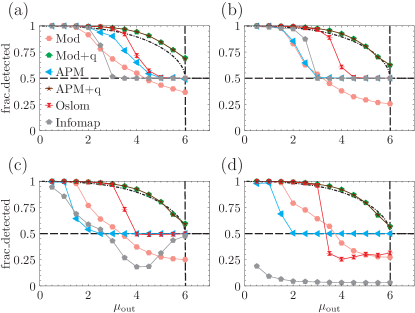
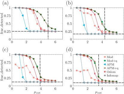
For Mod and APM we performed two types of runs, one without any indication on the number of clusters of the planted partition, the other by constraining the optimization procedure to partitions with clusters (Mod+q and APM+q). Fig. 1 shows that in general the performance of all methods is quite far from optimal. However, the limit performance (with slight variations due to finite size effects) is attained when the number of clusters of the planted partition is known. In particular, we remark that modularity maximization, in the absence of any information on the number of clusters, does a rather poor job. The limit curve and in general the whole analysis by Nadakuditi and Newman assumes that one knows the number of clusters beforehand, which is a very strong (and generally invalid) hypothesis. Furthermore, we observe that once the number of clusters is fixed to the correct value (in Mod+q and APM+q), both methods return the same results. Practically speaking, the only thing which a method can then do is move nodes to the cluster to which it has the most edges. The result is identical performance for any constant- method in this simple symmetric case. In Fig. 2, we see that knowledge of remains important as the number of clusters increases.
III Inferring the number of clusters from spectra of graph matrices
From Section II we conclude that knowing the number of clusters beforehand could push (some) methods up to the best attainable performance. Indeed, methods mostly fail in that they generally find a partition with a different number of clusters than the planted one. This is shown in Fig. 3, where we show the average number of clusters detected by the methods we used on the graphs of Fig. 1. For illustration purposes, we show the variable , where is the difference between the number of detected clusters and the actual number (here ). If , and =1. Naturally, Mod+q and APM+q yield the correct number of clusters by default, for any , since is given as input.
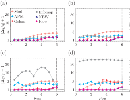
However, if the number of clusters is to be inferred by the method, it may differ from the actual at far below the detectability limit. In fact, for the largest graph sizes, deviations are large for very small values of , when the clusters of the planted partition are connected by very few links and should be easily distinguishable. In particular, we notice that Infomap, which is known to have an excellent performance on the more realistic LFR benchmark Lancichinetti and Fortunato (2009) breaks the two clusters in many pieces, so it is not a valuable predictor of for this graph model.
On the other hand, it has been recently shown that the correct number of clusters in the planted partition model can be correctly inferred from the spectra of two matrices: the non-backtracking matrix Krzakala et al. (2013) and the flow matrix Newman (2013). Both are matrices, where is the number of links of the network. Each link is considered in both directions, yielding directed links and indicated with the notation , meaning that the link goes from node to node . Their elements read
| (2) |
and
| (3) |
In Eq. 3 indicates the degree of node . So the elements of are basically the elements of , normalized by node degrees. This is done to account for the heterogeneous degree distributions observed in most real networks. Both matrices have non-zero elements only for each pair of links forming a directed path from the first node of one link to the second of the other link. To do that, links have to be incident at one node. As a matter of fact, the non-backtracking matrix is just the adjacency matrix of the (directed) links of the graph.
A remarkable property of both matrices is that most eigenvalues, which are generally complex, are enclosed by a circle centered at the origin, and that the number of eigenvalues lying outside of the circle is a good proxy of the number of communities of the network. For the circle’s radius is given by the square root of the leading eigenvalue ; for it equals , which is never greater than . In Refs. Krzakala et al. (2013) and Newman (2013) it was shown that the eigenvectors can be used for the detection of the communities, by turning the nodes into points in a -dimensional Euclidean space ( being the number of off-circle eigenvalues, i.e. of clusters), and grouping them with partitional clustering techniques, like K-means MacQueen (1967).
In Fig. 3 we added the predictions of the number of clusters obtained by both matrices (labeled by NBW and Flow). The exact techniques used to compute the spectra is listed in Appendix A. We find that the prediction is much more accurate than those of all community detection methods we used, and it becomes more precise, the larger the graph size, as expected. There is no difference between the two curves, because the degree of all nodes are essentially identical in the planted partition model, so the two matrices are basically proportional to one another and their spectra approximately coincide.
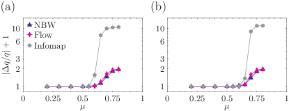
To see whether one can rely on the prediction of the number of clusters from the spectra of and , one should tackle more complex network models with communities. The classic version of the planted partition model, used here as well as in Refs.Krzakala et al. (2013); Newman (2013), is too homogeneous to resemble any real network. Nodes have approximately the same degree and communities have exactly the same size. The LFR benchmark graph Lancichinetti et al. (2008) is an extension of the planted partition model, where degrees and cluster sizes are distributed as power laws, as in many real systems. We want to see whether the number of clusters predicted by the non-backtracking and the flow matrices is as reliable on the LFR benchmark as it is on the classic model. This is shown in Fig. 4. The panels correspond to two different network sizes, and nodes, and two different ranges for the cluster sizes, S=small (communities comprise 10 to 50 nodes) and B = big (communities comprise 20 to 100 nodes). The mixing parameter is the ratio of the external degree of each node (with respect to the cluster it belongs to) by the total degree of the node, so it varies from to : values near zero correspond to well-separated clusters, whereas values near indicate a system with very mixed communities (hence hard to identify). The other parameters of the LFR benchmark are: average degree = , maximum degree = , degree distribution exponent = -2, cluster size distribution exponent = -1. The average number of clusters is (1000, S), (1000, B), (5000, S), (5000, B). These parameters are the same used for the comparative analysis of community detection algorithms of Ref. Lancichinetti and Fortunato (2009). Infomap was the best-performing method on those graphs, and this is reflected in Fig. 4, as it gives the best prediction of the number of clusters. Here the two matrices yield close but distinct results, due to the inhomogeneity of the degree distribution, but Infomap is clearly superior. We also remark that modularity optimization (Mod) fails to guess also for very low values of , due to the resolution limit Fortunato and Barthélemy (2007). So it seems that we do not gain that much by using and .
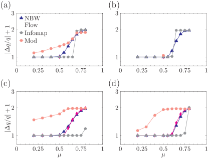
However, it may be that the situation improves on larger systems. Therefore, we repeated the procedure on two other sets of LFR graphs, with and nodes, respectively. We extended the range of cluster sizes to the interval , so that it spans two orders of magnitude and there is a big difference between the smallest and the largest community. All other graph parameters are the same as above. Here the average number of clusters is (10000), (20000). In Fig. 5 we show that in these larger and more heterogeneous graphs both the non-backtracking and the flow matrices give a better prediction of than Infomap.
IV A two-step approach
The results of Section III suggest that one might considerably improve the performance of community detection algorithms with a two-step procedure, in that one first infers the number of clusters through the spectrum of the non-backtracking or the flow matrix and then runs the algorithm on the space of partitions with that given number of clusters. Even if the inference of the correct number of clusters is not reliable, especially if the system is not too large, one might still get much closer to the true partition than by running the method without any information on the number of clusters.
To show that, we designed such two-step procedure for modularity optimization. The number of clusters is deduced through the flow matrix. Then, modularity is optimized via a greedy procedure, which exploits the idea of the Louvain algorithm Blondel et al. (2008). The latter works in a hierarchical manner. First, each node is its own cluster. Then nodes are put in the clusters of their neghbors such to yield the largest increase of modularity. This gives the first hierarchical level. Then such groups are turned into super-nodes and the procedure is repeated, which means that the clusters of the first hierarchical level are combined into larger groups, yielding the second hierarchical level, and so on, until one reaches the partition with largest modularity. Naturally, the number of clusters decreases when one moves from one level/partition to the next. We stop at the level such that the number of clusters is larger than the target number but the number of clusters of the level is smaller than . If by any chance there is a level such that we move to the refinement step described below. If there is no level such that , the algorithm is restarted with a different seed until such a partition is found. For the time being, we assume to be in the more frequent case in which we start with a partition with number of clusters larger than .
We then perform the following clean-up procedure in order to correct the number of communities, decreasing it to the correct value :
-
1.
Of all pairs of communities, choose the two which, when merged, give the greatest increase (least decrease) in the network modularity and merge them.
-
2.
Repeat (1) until the number of communities equals .
-
3.
Iterate through all nodes in random order. For each node, move it to the community which most increases modularity, or leave it in its present community if modularity can not be increased.
-
4.
Repeat (3) until there are no further changes to be made.
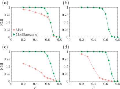
The last two steps are a refinement procedure aiming at further improving the modularity without changing the number of clusters, and are identical to the steps of our initial greedy procedure. In Fig. 6 we show the performance of this procedure on LFR benchmark graphs with the same parameters as the ones in Fig. 4 and those used in the comparative analysis of Ref. Lancichinetti and Fortunato (2009). As a reference, we report the performance curve of the exhaustive maximization of modularity via simulated annealing. We used simulated annealing because we wanted to get a very good estimate of the actual modularity maximum. Here the performance is expressed by the Normalized Mutual Information (NMI) Danon et al. (2005). We used the extended version of the NMI proposed by Lancichinetti et al. Lancichinetti et al. (2009), which can also compute the similarity of covers, i.e. of partitions of the network into overlapping communities. This version has been used consistently throughout the comparative analysis of Ref. Lancichinetti and Fortunato (2009). The two-step procedure introduced here outperforms the unconstrained exhaustive optimization of modularity, with the performance boost increasing for larger graphs. In Table 1 we show that the two-step algorithm has comparable complexity as simulated annealing.
| N | Spectral | Mod. | Infomap |
|---|---|---|---|
| 1000 | |||
| 5000 | |||
| 10000 | |||
| 20000 |
V Summary
We have seen that the number of clusters is an important input for community detection algorithms. If it is known beforehand, one can push up the performance of methods. We have shown that the spectra of the non-backtracking and flow matrices allow a reliable estimate of the number of clusters, both on the classic planted partition model and on the more realistic LFR benchmark, if the networks are not too small. Therefore, a two-step procedure, when one first derives the number of clusters and then performs a constrained run of the method one wishes to use, might lead to much better results. We have shown this for modularity optimization, whose unconstrained version preferentially leads to clusters of a given scale, which may or may not have anything to do with the actual scale of the clusters of the system at study. Instead, once the number of clusters is given, and the optimization is constrained on the set of partitions with that number of clusters, the method gives much better results.
In general, since the prediction of the number of clusters might not be correct, one could constrain the method on the set of partitions with number of clusters in a small range centered at the predicted value. This way, even if the actual value is missed but close, it can still be recovered by the procedure. It would be already valuable to “push” a method to the interesting range of values, instead of letting it free to be attracted somewhere else by intrinsic biases, as it happens for modularity.
On the practical side, computing the eigenvalues of the non-backtracking or the flow matrix is lengthy. Both are matrices. The adjacency matrix has elements, so and are larger by a factor of , where is the average degree of the network. Krzakala et al. have shown that the spectrum of can be computed by working on a matrix Krzakala et al. (2013), which reduces the complexity of the calculation by the factor . Still, an approximate but reliable computation of the spectra requires a time which scales approximately quadratically with the network size, by using standard software libraries (see Appendix). This is because the time needed to compute a single eigenvector/eigenvalue is linear in the graph size, but the number of clusters is proportional to , so the complexity of the calculation of eigenvectors/eigenvalues is approximately quadratic. Consequently, the problem is intractable for graphs with number of links of the order of millions or higher. This is the real bottleneck of the calculation. On the other hand, many systems of interest remain within reach. Besides, one could find other good predictors of the number of clusters which do not require lengthy calculations. In the example we have seen of the LFR benchmarks, Infomap is very good at guessing the right number of clusters and it runs much faster than the computation of the spectra of and . However, we have seen that it gives poor results on the classic planted partition model. Even if the latter is not a good model of real networks with community structure, it means that we should extensively test the reliability of a method before using it in applications. This manuscript shows that it might be a very good investment.
VI Acknowledgements
We thank Paolo De Los Rios, Lucio Floretta, Chris Moore, Lenka Zdeborova and Pan Zhang for useful exchanges. R. K. D. and S. F. gratefully acknowledge MULTIPLEX, grant number 317532 of the European Commission.
References
- Girvan and Newman (2002) M. Girvan and M. E. Newman, Proc. Natl. Acad. Sci. USA 99, 7821 (2002).
- Fortunato (2010) S. Fortunato, Physics Reports 486, 75 (2010).
- Krzakala et al. (2013) F. Krzakala, C. Moore, E. Mossel, J. Neeman, A. Sly, L. Zdeborová, and P. Zhang (2013), eprint ArXiv:1306.5550.
- Newman (2013) M. E. J. Newman (2013), eprint ArXiv:1308.6494.
- Condon and Karp (2001) A. Condon and R. M. Karp, Random Struct. Algor. 18, 116 (2001).
- Lancichinetti et al. (2008) A. Lancichinetti, S. Fortunato, and F. Radicchi, Phys. Rev. E 78, 046110 (2008).
- Newman (2004) M. E. J. Newman, Phys. Rev. E 69, 066133 (2004).
- Fortunato and Barthélemy (2007) S. Fortunato and M. Barthélemy, Proc. Natl. Acad. Sci. USA 104, 36 (2007).
- Good et al. (2010) B. H. Good, Y.-A. de Montjoye, and A. Clauset, Phys. Rev. E 81, 046106 (2010).
- Reichardt and Leone (2008) J. Reichardt and M. Leone, Phys. Rev. Lett. 101, 078701 (2008).
- Decelle et al. (2011a) A. Decelle, F. Krzakala, C. Moore, and L. Zdeborová, Phys. Rev. Lett. 107, 065701 (2011a).
- Decelle et al. (2011b) A. Decelle, F. Krzakala, C. Moore, and L. Zdeborová, Phys. Rev. E 84, 066106 (2011b).
- Nadakuditi and Newman (2012) R. R. Nadakuditi and M. E. J. Newman, Phys. Rev. Lett. 108, 188701 (2012).
- Floretta et al. (2013) L. Floretta, J. Liechti, A. Flammini, and P. De Los Rios, Phys. Rev. E 88, 060801(R) (2013).
- Guimerà et al. (2004) R. Guimerà, M. Sales-Pardo, and L. A. Amaral, Phys. Rev. E 70, 025101 (R) (2004).
- Ronhovde and Nussinov (2010) P. Ronhovde and Z. Nussinov, Phys. Rev. E 81, 046114 (2010).
- Lancichinetti et al. (2011) A. Lancichinetti, F. Radicchi, J. J. Ramasco, and S. Fortunato, PLoS ONE 6, e18961 (2011).
- Rosvall and Bergstrom (2008) M. Rosvall and C. T. Bergstrom, Proc. Natl. Acad. Sci. USA 105, 1118 (2008).
- Lancichinetti and Fortunato (2009) A. Lancichinetti and S. Fortunato, Phys. Rev. E 80, 056117 (2009).
- MacQueen (1967) J. B. MacQueen, in Proc. of the fifth Berkeley Symposium on Mathematical Statistics and Probability, edited by L. M. L. Cam and J. Neyman (University of California Press, Berkeley, USA, 1967), vol. 1, pp. 281–297.
- Blondel et al. (2008) V. D. Blondel, J.-L. Guillaume, R. Lambiotte, and E. Lefebvre, J. Stat. Mech. P10008 (2008).
- Danon et al. (2005) L. Danon, A. Díaz-Guilera, J. Duch, and A. Arenas, J. Stat. Mech. P09008 (2005).
- Lancichinetti et al. (2009) A. Lancichinetti, S. Fortunato, and J. Kertesz, New J. Phys. 11, 033015 (2009).
- Newman (2006) M. E. J. Newman, Proc. Natl. Acad. Sci. USA 103, 8577 (2006).
- Guimerà and Amaral (2005) R. Guimerà and L. A. N. Amaral, Nature 433, 895 (2005).
- Landau and Binder (2005) D. Landau and K. Binder, A Guide to Monte Carlo Simulations in Statistical Physics (Cambridge University Press, New York, NY, USA, 2005), ISBN 0521842387.
- Ronhovde and Nussinov (2009) P. Ronhovde and Z. Nussinov, Phys. Rev. E 80, 016109 (2009).
- Jones et al. (2001–) E. Jones, T. Oliphant, P. Peterson, et al., SciPy: Open source scientific tools for Python (2001–), URL http://www.scipy.org/.
- Lehoucq et al. (1998) R. R. B. Lehoucq, D. D. C. Sorensen, and C.-C. Yang, Arpack User’s Guide: Solution of Large-Scale Eigenvalue Problems With Implicityly Restorted Arnoldi Methods, vol. 6 (SIAM, 1998).
- Lehoucq and Sorensen (1996) R. B. Lehoucq and D. C. Sorensen, SIAM Journal on Matrix Analysis and Applications 17, 789 (1996).
Appendix A Methods
In this section, we describe the community detection methods and used in this work and their respective parameters.
A.1 Modularity
Network modularity is measure which rates the quality of a network partition, with higher modularity presumably indicating better communities. Modularity compares the actual number of intra-community links to the expected number of links in a random graph with the same degree distribution. The details of modularity optimization have been extensively described in other work, for example Newman (2006). We adopt a simulated annealing approach in the spirit of Guimerà and Amaral (2005). The Hamiltonian formulation of modularity reads
| (4) |
with if there is an edge between nodes and and zero otherwise, , the degrees of nodes and respectively, the total number of (non-directed) edges of the graph, , the respective community of nodes and , and the Kronecker delta function. A variety of trial moves are applied, and accepted according to the Metropolis criteria Landau and Binder (2005):
-
•
Shift moves: A node may be shifted from one community to another (possibly empty) community. This may possibly result in the number of communities decreasing or increasing if the node is moved to a new community or was previously in a singleton community.
-
•
Merge moves: Two randomly selected communities are selected and merged.
-
•
Split moves: A community is chosen at random and split. When splitting, each node has an equal and independent probability of to join the new community being formed by the split. A more sophisticated method could run community detection within the community in order to determine the optimal community split.
Mod: For regular modularity calculations, first all nodes are assigned to singleton communities (every node in its own distinct community), and the Hamiltonian/energy is calculated from Eq. 4. Then, for each round, we do one trial move of each node into a different random community ( moves). Then, there is one merge move between two random communities, and one split move of a random community. After every round, the network modularity is calculated and configuration is stored if the current partition is better than the previously optimal partition. We choose an initial temperature , and after each round, temperature is updated via . Trials continue until energy does not decrease by more than for 1000 rounds. This entire procedure is repeated 5 times for each graph, and the lowest energy result of all trials is selected as the final partition. We achieved 100 averages for all points with these parameters.
Mod+q: This procedure, used in Figs. 1-3, uses simulated annealing with an additional term and different parameters to fix the number of clusters to , the true number of communities. The Hamiltonian (note different normalization) is
| (5) |
with
| (6) |
being the term to fix . We choose . Thus, as temperature decreases, the number of clusters becomes energetically fixed at the true number. The initial configuration is set with all nodes divided randomly among clusters, though may fluctuate during the minimization. Each round consists of moves, with , , and for each move. We choose an initial temperature , and after each round, temperature is decreased by a factor . Trial rounds continue, until there are no more changes accepted for 10 rounds. This procedure is repeated 10 times per graph, with the lowest final energy being taken as the final partition. We achieved 100 averaging runs for all points with these parameters.
A.2 Absolute Potts Model (APM)
The APM detects communities via minimization of a Hamiltonian without a null model,
| (7) |
where is the inverse adjacency matrix. In addition, is a resolution parameter which can be varied across a range of values in order to determine the optimal community size. The optimal is inferred by the self-similarity of multiple greedy trial minimizations performed on the same graph. We use the classic normalized mutual information Danon et al. (2005) to select the optimal , and in general follow the procedure of Ref. Ronhovde and Nussinov (2009). We achieved 100 averaging runs for all points with these parameters.
APM+q: For constant- APM runs, we do not use the multi-resolution procedure of the previous paragraph. Instead, we fix and use the constant- simulated annealing procedure described under Mod+q above, but with the APM Hamiltonian plus term. We achieved 100 averaging runs for all points with these parameters.
A.3 Oslom
The Order Statistics Local Optimization Method (OSLOM) method seeks statistically significant clusters in networks. We use the OSLOM code available at http://oslom.org/. All default parameters are accepted, but in addition we enable the option to ensure that all nodes are a member of at least one community (no homeless nodes, the default in the latest released code), which is sensible for the case where all nodes are contained in at least one community. The default of 10 trial optimizations of the lowest hierarchical level is used, and the lowest hierarchical level is selected as the resulting partition. All Oslom data is averaged over 100 graph realizations unless otherwise indicated.
A.4 Infomap
Infomap is a method based on the compression of a random walk on graphs. The source code can be downloaded at http://mapequation.org/. All default options are accepted, but notably we restrict the algorithm to a single non-hierarchical partition (--two-level) and request ten trial minimizations for each graph. All Infomap data is averaged over 100 graph realizations unless otherwise indicated.
A.5 Spectral methods
For a description of the non-backtracking walk and flow matrices, see Sec. III. We use a home-build implementation of these methods, as described in Refs. Krzakala et al. (2013); Newman (2013). Actual eigenvalue computation is via the scipy sparse linear algebra package Jones et al. (2001–), which is an interface to the ARPACK library Lehoucq et al. (1998), which itself uses the implicitly restarted Arnoldi method for computing eigenvalues Lehoucq and Sorensen (1996). In order to infer that a graph has communities, we must compute at least eigenvalues ( eigenvalues outside of the circle, and one inside of the circle to know that the calculation is finished). All spectral data is averaged over 100 graph realizations unless otherwise indicated. The time taken to compute eigenvalues scales as , as is generally a function of (approximately linear). All spectral data is averaged over 100 graph realizations unless otherwise indicated. Some actual times to compute these eigenvalues are shown in Table 2.
| N | Flow EV calc. | Mod. | Infomap | Mod. known |
|---|---|---|---|---|
| 1000 | ||||
| 5000 | ||||
| 10000 | ||||
| 20000 |