Valence bond distribution and correlation in bipartite Heisenberg antiferromagnets

Abstract

Every singlet state of a quantum spin-$1/2$ system can be decomposed into a linear combination of valence bond basis states. The range of valence bonds within this linear combination as well as the correlations between them can reveal the nature of the singlet state, and are key ingredients in variational calculations. In this work, we study the bipartite valence bond distributions and their correlations within the ground state of the Heisenberg antiferromagnet on bipartite lattices. In terms of field theory, this problem can be mapped to correlation functions near a boundary. In dimension $d\geq 2$, a non-linear $\sigma$ model analysis reveals that at long distances the probability distribution $P({\bf r})$ of valence bond lengths decays as $|r|^{-d-1}$ and that valence bonds are uncorrelated. By a bosonization analysis, we also obtain $P({\bf r})\propto|r|^{-d-1}$ in $d=1$ despite the different mechanism. On the other hand, we find that correlations between valence bonds are important even at large distances in $d=1$, in stark contrast to $d\geq 2$. The analytical results are confirmed by high-precision quantum Monte Carlo simulations in $d=1$, $2$ and $3$. We develop a single-projection loop variant of the valence bond projection algorithm, which is well designed to compute valence bond probabilities and for which we provide algorithmic details.

I Introduction

Magnetic ordering is a primary concern of classical magnetism. Long-range order can be disrupted by the presence of disorder or of frustration between the magnetic degrees of freedom. Quantum fluctuations form also an important path to destroy long-range order, specifically antiferromagnetic (AF) order. They are particularly strong for low values of the spin $S$ and in low dimensionality. The prototypical model to study quantum fluctuations is the $S=1/2$ AF Heisenberg model

$${\cal H}=\sum_{\langle i,j\rangle}{\bf S}_{i}\cdot{\bf S}_{j},$$ (1)

where ${\langle i,j\rangle}$ denote nearest-neighbor (NN) sites on a hypercubic lattice, and ${\bf S}_{i}$ the spin operator [of amplitude ${{\bf S}_{i}}^{2}=S(S+1)$] on site $i$. While long-range order in the ground state of Eq. (1) is prohibited in one dimension (1D) BetheMerminWagner , it can be shown rigorously LRO that the system displays long-range order in $d=2$ for all $S\geq 1$. For $S=1/2$, there is no exact proof but the numerical computations NumLRO ; SandvikEvertz leave no doubt that this is also the case. In this paper, we deal only with this extreme quantum case $S=1/2$ and assume an even number $N$ of spins.

The Hamiltonian Eq. (1) exhibits SU(2) symmetry, as it commutes with the total spin operator ${\bf S}_{T}=\sum_{i=1}^{N}{\bf S}_{i}$. The total spin quantum number $S_{T}$ is defined by the eigenvalue $S_{T}(S_{T}+1)$ of the operator ${{\bf S}_{T}}^{2}$. For AF interactions, the ground state for finite $N$ of the Hamiltonian Eq. (1) on the hypercubic lattice can be proven LiebMattis to be a total singlet $S_{T}=0$. Natural objects to describe such a singlet state are valence bonds (VBs), which are intrinsically non-magnetic and antisymmetric objects, with two spins $1/2$ coupled into a singlet. This notion was introduced in the early days of quantum mechanics old and has regained interest thanks to the proposal that wave functions composed of VBs [“resonating valence bond (RVB) wave functions”] could describe a quantum spin-liquid phase without any magnetic order, for Heisenberg models on frustrated lattices Anderson . The idea is that local (typically NN) superpositions of VBs can effectively accommodate the constraint imposed by frustration in the building blocks of such lattices and lower the energy of the full system. While the original suggestion Anderson of this scenario taking place on the triangular lattice is now abandoned (since this lattice supports AF long-range order TriangularLRO ), it stimulated many investigations which led to significant progresses in quantum magnetism. In fact, the existence of the RVB phase is established in several quantum dimer models MoessnerSondhi ; MisguichSerbanPasquier , which are effective models of quantum antiferromagnets. Furthermore, the usefulness of VB wave functions has been demonstrated for the understanding of the low-energy physics of Heisenberg AF models on other frustrated lattices, such as kagome kagome or frustrated square lattices Mambrini06 ; LouSandvik ; Zhang13 . These developments have confirmed the importance of the VB picture in understanding quantum antiferromagnets.

Much of the studies of quantum antiferromagnets based on the VB picture is aimed at quantum spin liquids without a long-range antiferromagnetic order. However, it should be noted that the set of VB states, once including longer-range VBs beyond nearest neighbors, is overcomplete in the total singlet sector old ; old2 . Thus, any singlet state can be represented as a superposition of VB basis states. The finite-size ground state of the antiferromagnetic Hamiltonian on the hypercubic lattice in $d\geq 2$ dimensions is no exception, despite its long-range antiferromagnetic order. This somewhat counterintuitive fact is indeed consistent with the existence of symmetry-broken ground states in the thermodynamic limit, thanks to the asymptotic degeneracy in the thermodynamic limit $N\to\infty$ of the “Anderson tower of states” of nonzero total spin $S_{T}$ with the ground state AndersonBook .

An antiferromagnet is called a bipartite antiferromagnet if the sites can be grouped into two sublattices, and the Heisenberg exchange interactions exist only between two sites belonging to different sublattices. Examples include the antiferromagnets on a hypercubic lattice with only nearest-neighbor interactions. It is then natural to consider a restricted set of VB basis states, bipartite VB basis states, in which only VBs connecting different sublattices are allowed BeachSandvik . Even the bipartite VB basis, if longer-range VBs are included, is overcomplete in the total singlet sector (see e.g. Ref. BeachSandvik, or Ref. Mambrini, ) and thus can represent any singlet ground state of an $S=1/2$ antiferromagnet. In fact, in a pioneering work by Liang, Douçot and Anderson (LDA) LDA , the long-range-ordered AF ground state of the Heisenberg antiferromagnet on the square lattice was described in terms of bipartite VB basis states, including bipartite VBs of arbitrary length. In practice, this was done by defining a so-called amplitude product state, where the weight of every valence bond state is factorized into weights $h({\bf r})$ coming from contributing valence bonds of length ${\bf r}$. The original results of LDA pointed to a minimal variational energy for the square lattice Heisenberg model reached for a power law decay $h(r)\propto r^{-\alpha}$, with $\alpha\approx 4$.

The VB basis provides a new perspective for understanding quantum antiferromagnets, which is complementary to the more traditional $S^{z}$ basis. As an indication of its significance, a quantum Monte Carlo (QMC) algorithm based on the VB basis was proposed Sandvik05 and proved to be useful. The more recent numerical results from the VB-based QMC simulation Sandvik05 , obtained without assuming the power-law decay, imply $\alpha=3$ rather than $\alpha\sim 4$ suggested by LDA. This power-law decay and the value $\alpha=3$ can be understood through a master equation BeachMaster or other mean-field Beach ; Wegner approaches, which moreover predict $\alpha=d+1$ to be the best variational ansatz for the ground state of Eq. (1) in dimension $d$, within amplitude product states. These previous works were explicitly assuming a certain amplitude product variational ansatz for the antiferromagnetic ground state note-beach . However, one could instead also ask for the length distribution $P({\bf r})$ of valence bonds in the real ground state of Heisenberg antiferromagnets. This question may at first glance seem ill defined since the expression of singlet states in terms of valence bonds is in general non-unique. Fortunately, the occupation number of bipartite valence bonds is nevertheless still well defined Mambrini ; Alet10 .

In this paper, we compute by analytical means the distribution of VB lengths $P({\bf r})$ for antiferromagnetic Heisenberg models on hypercubic lattices in dimension $d$. Somewhat surprisingly, the question of VB distribution can be reduced to a problem of boundary field theory. YellowPages ; BlumenhagenPlauschinn Boundary field theory has been found useful, not only in boundary critical phenomena and quantum impurity problems, but also in recent topics such as entanglement entropy. FradkinMoore ; MO-EE-BCFT ; JacobsenSaleur ; StephanMisguichPasquier The VB distribution may be added to the list of applications of boundary field theory. The key in the relation is the identity Alet10 between the bipartite VB distribution and an overlap with the reference state, which is naturally related to boundary correlation functions.

In principle, any field theory, which is an appropriate effective theory for the bulk, can be used to calculate the bipartite VB distribution with a certain boundary condition. The ground state and low-energy excitations of the Heisenberg antiferromagnet on the hypercubic lattice in $d\geq 2$ spatial dimensions are believed to be described by the O(3) non-linear $\sigma$ model. In fact, in the ground state, the SU(2) symmetry is spontaneously broken in the non-linear $\sigma$ model in $d\geq 2$, as is the case in the Heisenberg antiferromagnet on the hypercubic lattice. The effective field theory in the low-energy limit is then reduced to the field theory of two massless Nambu-Goldstone modes. We will apply such a field theory with boundary, in order to study the bipartite VB distribution in $d\geq 2$ dimensions.

On the other hand, in $d=1$, the physics is quite different as there is no spontaneous breaking of the symmetry. The system belongs to the universality class of Tomonaga-Luttinger liquids, which can be described by a free-boson field theory in $d=1$ spatial dimension. Again, together with an appropriate boundary condition, it is applied to the bipartite VB distribution in $d=1$ dimension. As a result, in $d\geq 1$ dimensions, we find a power-law dependence $P({\bf r})\propto|{\bf r}|^{-(d+1)}$, confirming previous results based on mean-field approximations Wegner ; Beach ; BeachMaster as well as a previous numerical QMC estimate Sandvik05 . The analytical predictions are compared in detail to the results of QMC simulations of the Heisenberg model in dimension $d=1$, 2 and 3.

While “free-boson field theory” is a common ingredient for the cases $d=1$ and $d\geq 2$, the correspondence between the field theory and the quantum antiferromagnet is quite different, reflecting the very different physics. In fact, the difference between $d=1$ and $d\geq 2$ becomes apparent in the correlations between VBs, as follows. In the wave function studied by LDA, it is assumed that the weight of each VB configuration can be factorized in products of weights carried by each VB individually:

$$|\Psi_{\rm LDA}\rangle=\sum_{c}w_{c}|c\rangle,$$ (2)

$${\rm with\quad}w_{c}=\prod_{(i,j)\in c}h_{ij},$$

where $c$ denotes a VB configuration composed of different VBs $(i,j)$ formed between spins at sites $i$ and $j$. The amplitude $h_{ij}$ is often chosen as depending on the distance $r_{ij}$ between $i$ and $j$, i.e., the “length” of the VB $(i,j)$. The factorization of VB amplitudes means the absence of correlation among VBs. It is indeed a strong assumption in the ansatz LDA wave function, and very few works HuseElser to our best knowledge went beyond it until recently BeyondLDA ; Lin12 ; Zhang13 . In fact, it is very natural to ask whether this assumption is correct or can be justified for realistic (short-range) Heisenberg models.

The boundary field theory approach allows us to elucidate analytically the correlation among VBs. We find that, whereas there are nontrivial correlations between VB occupation numbers even at large distances for $d=1$, no correlations are asymptotically present in $d\geq 2$. The analytical prediction is then carefully verified via a numerical investigation with QMC simulations. This difference between $d=1$ and $d\geq 2$ is another manifestation of different physics, in terms of the VB picture. Our results for $d\geq 2$ also justify the use of factorized wave functions of the LDA type.

The plan of the paper is the following. In Sec. II, we review the notion of valence bond occupation and correlation in a singlet wave function, giving a pedagogical derivation of a simple formula to effectively count the “average” number of VBs shared by two sites. In Sec. III, we present a method to measure these quantities numerically using QMC algorithms in the VB basis, and discuss in particular a specific improved algorithm for doing so. We then consider the case of $d\geq 2$ Heisenberg antiferromagnets using a non-linear $\sigma$ model description in Sec. IV.1, computing the VB length distribution as well as correlations. We furthermore compare the analytical predictions for the Heisenberg model on the square and simple cubic lattices with QMC results. In Sec. V.1, we study the more complicated case (from the analytical point of view) of $d=1$ with bosonization, showing the presence of correlations between VBs. The numerical computations in $d=1$ are simpler and allow for an exhaustive comparison with bosonization results. We further discuss the implication of our results in Sec. VI and give a conclusion.

II Definition

Figure 1: (Color online) a) The reference Néel state (on a one-dimensional lattice) with all spins pointing up (down) on sublattice $A$ ($B$) has on overlap of $2^{-N/4}$ with all bipartite valence bond states, since each of the $N/2$ valence bonds contributes with a factor $1/\sqrt{2}$. b) Swapping the spins of the Néel state in region ${\cal S}_{A}$ with those in region ${\cal S}_{B}$ creates a reference state, which has a slightly different overlap with bipartite valence bond states. Every valence bond connecting ${\cal S}_{A}$ and ${\cal S}_{B}$ contributes a factor of $-1/\sqrt{2}$, whereas bipartite valence bonds, being only connected to one of the swapped regions, contribute a factor $0$. Depending on the size of the swapped regions, one can thus measure the single VB occupations ($|{\cal S}_{A}|=1=|{\cal S}_{B}|$), simultaneous occupations of two VBs ($|{\cal S}_{A}|=2=|{\cal S}_{B}|$), and others.

Consider a bipartite lattice, such that interactions in the Hamiltonian Eq. (1) occur only between sublattice $A$ and sublattice $B$. Every bipartite valence bond state $\left|\varphi_{\alpha}\right>$ on such a lattice may be written as

$$\left|\varphi_{\alpha}\right>=\left|(i_{1},j_{1})(i_{2},j_{2})\cdots(i_{N/2},j_{N/2})\right>,$$ (3)

with $i_{k}\in{\cal A}$ on sublattice $A$ and $j_{k}\in{\cal B}$ on sublattice $B$. In this notation the pairs $(k,l)$ represent precisely the bipartite valence bonds

$$\left|(k,l)\right>=\frac{\left|\uparrow_{k}\downarrow_{l}\right>-\left|\downarrow_{k}\uparrow_{l}\right>}{\sqrt{2}},$$ (4)

that form the state $\left|\varphi_{\alpha}\right>$. We may then define the occupation number $n_{k,l}$ of a valence bond state as

$$n_{k,l}(\left|\varphi_{\alpha}\right>)=\left\{\begin{array}[]{lll}1&\mbox{if }(k,l)\in\left|\varphi_{\alpha}\right>,\\ 0&\mbox{otherwise}.\end{array}\right.$$ (5)

Note, that this definition is rather formal and not always very useful. Using the Néel state

$$\left|\mbox{N\'{e}el}\right>=\prod_{i\in{\cal A}}\left|\uparrow_{i}\right>\prod_{j\in{\cal B}}\left|\downarrow_{j}\right>,$$ (6)

an interesting alternative expression can be given in the form of a scalar product Alet10 :

$$n_{k,l}(\left|\varphi_{\alpha}\right>)=-\frac{\left<\mbox{N\'{e}el}\middle|S_{k}^{+}S_{l}^{-}\middle|\varphi_{\alpha}\right>}{\left<\mbox{N\'{e}el}\middle|\varphi_{\alpha}\right>}.$$ (7)

Therein, the operator $S_{l}^{+}S_{k}^{-}$ permutes the spins $k$ and $l$ within the Néel state $\left|\mbox{N\'{e}el}\right>$, as illustrated in Fig. 1. Notice that here we swap only a single spin ($|{\cal S}_{A}|=1=|{\cal S}_{B}|$), with ${\cal S}_{A}=\{k\}$ and ${\cal S}_{B}=\{l\}$. Obviously, a valence bond $(k,l)$ in $\left|\varphi_{\alpha}\right>$ contributes a factor of $1/\sqrt{2}$ when overlapped with $\left<\uparrow_{k}\downarrow_{l}\right|$ and $-1/\sqrt{2}$ for the overlap with $\left<\downarrow_{k}\uparrow_{l}\right|$. Hence, a valence bond connecting ${\cal S}_{A}$ and ${\cal S}_{B}$ must yield a factor of $1$ in Eq. (7), as required. On the other hand, if there are valence bonds $(k,m)$ that connect ${\cal S}_{A}$ and ${\cal B}-{\cal S}_{B}$ (see Fig. 1), then the overlap with a triplet state vanishes $\left<\downarrow_{k}\downarrow_{m}\middle|(k,m)\right>=0$, thus showing the equivalence of Eq. (7) with Eq. (5).

It is also straightforward to generalize Eq. (7) to arbitrary singlet states Alet10 ; Mambrini , which can always be expressed as (albeit non-unique) superpositions of bipartite VB states. Writing a given singlet state $|\Psi\rangle$ as

$$\left|\Psi\right>=\sum_{i}a_{i}\left|\varphi_{i}\right>,$$ (8)

we can immediately generalize Eq. (7) to the “average” VB occupation number for $|\Psi\rangle$ as

$$\bar{n}_{(k,l)}(\left|\Psi\right>)=-\frac{\left<\mbox{N\'{e}el}\middle|S_{k}^{+}S_{l}^{-}\middle|\Psi\right>}{\left<\mbox{N\'{e}el}\middle|\Psi\right>}.$$ (9)

Even though the expression Eq. (8) of the singlet state in terms of VB basis states is not unique, the VB occupation number Eq. (9) is unique and well defined. Since every VB basis state has the same overlap with the Néel state, that is, $\left<\mbox{N\'{e}el}\middle|\varphi_{i}\right>=2^{-N/4}$, Eq. (9) is thus an “average” defined with respect to the coefficients $a_{i}$ themselves as the weight, and not to their squares $|a_{i}|^{2}$. If some of the coefficients $a_{i}$ can be negative, the average Eq. (9) may be ill defined. However, for the ground state of a bipartite quantum antiferromagnet, all the coefficients $a_{i}$ of the bipartite VB basis states are non-negative upon a proper choice of the overall phase factor, thanks to Marshall’s sign rule Marshall ; LDA . Thus the average occupation number is always well-defined for such a ground state and satisfies $0\leq\bar{n}_{(k,l)}\leq 1$. We emphasize that this only applies to bipartite valence bonds Mambrini ; Alet10 .

We define the single VB distribution function

$$P(\mathbf{r})\equiv\bar{n}_{(k,l)},$$ (10)

where two sites $k,l$ are separated by the vector $\mathbf{r}$. As we consider translationally invariant systems, $\bar{n}_{k,l}$ should not depend on the choice of the site $k$ and is a function of the separation ${\bf r}$ only. Moreover, since the site $k$ must belong to one VB in any of the VB basis states, we find the sum rule

$$\sum_{\mathbf{r}}P(\mathbf{r})=1.$$ (11)

This construction carries over immediately to the more general problem of simultaneous occupation numbers of multiple VBs. This can be done by choosing the set of sites ${\cal S}_{A}$ and ${\cal S}_{B}$ from each sublattice $A$ and $B$, so that $|{\cal S}_{A}|=|{\cal S}_{B}|>1$. Then, the “number of VBs connecting ${\cal S}_{A}$ and ${\cal S}_{B}$” can be obtained as

$$\bar{n}_{{\cal S}_{A},{\cal S}_{B}}(\left|\Psi\right>) =-\frac{\left<\mbox{N\'{e}el}\middle|\prod_{k\in{\cal S}_{A}}S_{k}^{+}\prod_{l\in{\cal S}_{B}}S_{l}^{-}\middle|\Psi\right>}{\left<\mbox{N\'{e}el}\middle|\Psi\right>}$$

$$=-\frac{\sum_{i}a_{i}\left<\mbox{N\'{e}el}\middle|\prod_{k\in{\cal S}_{A}}S_{k}^{+}\prod_{l\in{\cal S}_{B}}S_{l}^{-}\middle|\varphi_{i}\right>}{\sum_{i}a_{i}\left<\mbox{N\'{e}el}\middle|\varphi_{i}\right>}.$$ (12)

We note that, in this quantity, one no longer sees which sites precisely in ${\cal S}_{A}$ and ${\cal S}_{B}$ are connected to each other. For example, with the choice of ${\cal S}_{A}=\{k,l\}$ and ${\cal S}_{B}=\{m,n\}$, we measure the simultaneous occupation of two VBs connecting the two sets. This may be interpreted as a sum of the occupation numbers for the two possible VB configurations $\left|(k,m)(l,n)\right>$ and $\left|(k,n)(l,m)\right>$:

$$\bar{n}_{\{k,l\},\{m,n\}}(\left|\Psi\right>) =\bar{n}_{(k,m)(l,n)}(\left|\Psi\right>)+\bar{n}_{(k,n)(l,m)}(\left|\Psi\right>)$$

$$=-\frac{\left<\mbox{N\'{e}el}\middle|S_{k}^{+}S_{l}^{+}S_{m}^{-}S_{n}^{-}\middle|\Psi\right>}{\left<\mbox{N\'{e}el}\middle|\Psi\right>}.$$ (13)

We assert that, however, the occupation numbers for the individual VB configurations $\left|(k,m)(l,n)\right>$ or $\left|(k,n)(l,m)\right>$ are not well defined, and only the combination Eq. (13) is uniquely defined.

III Measuring valence bond occupations and correlations in Quantum Monte Carlo simulations

Measuring valence bond occupation numbers or correlations is straightforward using Eq. (II) if one has direct access to the wave function studied, such as within exact diagonalization or density matrix renormalization group (DMRG) calculations (see Ref. Alet10, for a more precise discussion and an example of such computations). Since, however, we would like to study asymptotic, long-distance, properties of $d>1$ quantum antiferromagnets on large systems, these methods are not practical and we have to resort to stochastic QMC schemes.

III.1 General statements on valence bond QMC

Recent QMC state-of-the-art algorithms allow access to quantities in the valence bond language directly, by projecting out the ground state from some trial wave function. The trial wave function is usually chosen to be some special singlet state, such as the amplitude product state Eq. (2), in order to achieve a significant reduction of computational cost SandvikBeach .

Initially, two such schemes have been devised Sandvik05 , which are often referred to as single projection and double projection, respectively. The choice between these two schemes depends on the observable we want to measure. Observables that commute with the Hamiltonian can be measured within the single projection scheme, where some power $m$ of the Hamiltonian ${\cal H}$ is applied to a singlet trial state $\left|\Psi_{\rm in}\right>$,

$$\left<{\cal O}\right>=\frac{\left<\mbox{R}\right|{\cal O}(C-{\cal H})^{m}\left|\Psi_{\rm in}\right>}{\left<\mbox{R}\right|(C-{\cal H})^{m}\left|\Psi_{\rm in}\right>}.$$ (14)

Herein, $\left|\mbox{R}\right>$ is a reference state, which is in principle arbitrary. However, it turns out that the Néel state $\left|\mbox{{N\'{e}el}}\right>$ is a particularly good choice, as it has the same overlap with all singlet states. Furthermore, $C$ is chosen to be the energy of the maximally polarized state $\left|\uparrow\cdots\uparrow\right>$, such that the projection reveals the ground state.

Notice, that such a scheme requires the ground state $(C-{\cal H})^{m}\left|\Psi_{\rm in}\right>$ to be an eigenstate of the observable ${\cal O}$. In cases where this does not apply we have to carry out the double projection scheme, where the ground state projection occurs on both sides,

$$\left<{\cal O}\right>=\frac{\left<\Psi_{\rm in}\right|(C-{\cal H})^{m}{\cal O}(C-{\cal H})^{m}\left|\Psi_{\rm in}\right>}{\left<\Psi_{\rm in}\right|(C-{\cal H})^{2m}\left|\Psi_{\rm in}\right>}.$$ (15)

Valence bond occupation, Eq. (II), is a rather peculiar quantity, which measures properties of a given singlet state without being an observable. There are however different ways to generate related observables, which can be measured within double projection, e.g.,

$${\cal O}_{k,l} =S_{k}^{-}S_{l}^{+}\left|\mbox{N\'{e}el}\middle>\middle<\mbox{N\'{e}el}\right|S_{k}^{+}S_{l}^{-},$$ (16)

$${\cal P}_{k,l} =-\frac{1}{2}\left(\left|\mbox{N\'{e}el}\middle>\middle<\mbox{N\'{e}el}\right|S_{k}^{+}S_{l}^{-}+S_{k}^{-}S_{l}^{+}\left|\mbox{N\'{e}el}\middle>\middle<\mbox{N\'{e}el}\right|\right).$$ (17)

Unfortunately, it turns out that simulations converge rather badly when carrying out a double projection scheme with these observables. This is due to the fact that the appropriate estimator fluctuates exponentially, like the one for fidelity Schwandt09 and Rényi entropies Hastings10 and in contrast to the energy estimator and other quantum mechanical observables Sandvik05 .

On the other hand, one notices that Eq. (II) looks very similar to the single projection expression Eq. (14), suggesting an implementation of this last scheme. Indeed valence bond occupations (through the related valence bond entanglement entropy vbee ) have already been measured with the single projection method using a local update algorithm. However, whereas for the double projection method very efficient loop updates are known SandvikEvertz , this seems not to be the case for the single projection algorithm. We devote the next section to the description of such a method.

III.2 Single projection QMC algorithm with loop updates

In order to carry out a single projection scheme, we first rewrite expression Eq. (14) and decompose the projection step as a sum over all possible contributing bond operator strings Sandvik05 ; SandvikEvertz

$$(C-{\cal H})^{m}=\sum_{r}{P}_{r}^{(m)}.$$ (18)

Every one of such operator strings is a product of bond singlet projectors,

$${P}_{r}^{(m)}={\cal P}_{b_{1}}^{(s=0)}\cdots{\cal P}_{b_{m}}^{(s=0)},$$ (19)

and $r=(b_{1},\ldots,b_{m})$ is a multi-index that is summed over. Notice, that the singlet projector ${\cal P}_{b}^{(s=0)}$ on a given bond $b=\,\langle i,j\rangle$ between sites $i$ and $j$ is related to the spin-spin interaction by

$${\cal P}_{\langle i,j\rangle}^{(s=0)}=\frac{1}{4}-{\bf S}_{i}\cdot{\bf S}_{j}.$$ (20)

With these notations and noting that the singlet trial state can be decomposed as a superposition of bipartite VB states $\left|\Psi_{\rm in}\right>=\sum_{i}a_{i}\left|\varphi_{i}\right>$, Eq. (14) reads

$$\left<{\cal O}\right>=\frac{\sum_{r,i}a_{i}\left<\mbox{{N\'{e}el}}\right|{\cal O}{P}_{r}^{(m)}\left|\varphi_{i}\right>}{\sum_{r,i}a_{i}\left<\mbox{{N\'{e}el}}\right|{P}_{r}^{(m)}\left|\varphi_{i}\right>},$$ (21)

where $\left|\mbox{{N\'{e}el}}\right>$ is used as the reference state and the sums over $r$ and $i$ can be sampled stochastically. The way this is done is illustrated in Fig. 2, where an example bond operator string is explicitly written out. We use the following updates in order to sample the configuration space of different bond operator positions and valence bond states.

Figure 2: (Color online) Schematic representation of the expression $\left<\uparrow\downarrow\uparrow\downarrow\right|{\cal P}_{\langle 2,3\rangle}^{(s=0)}{\cal P}_{\langle 1,2\rangle}^{(s=0)}{\cal P}_{\langle 3,4\rangle}^{(s=0)}{\cal P}_{\langle 2,3\rangle}^{(s=0)}{\cal P}_{\langle 1,2\rangle}^{(s=0)}\left|(1,2)(3,4)\right>$, residing on $N=4$ sites (drawn vertically). Herein, the singlet projectors (red shaded squares) are intentionally represented by two valence bonds. Notice that the Néel state on the left (represented by black and white circles) does not close the red (dashed) loops, whereas the blue (continuous) loops are closed intrinsically or by the valence bond state (yellow shaded rectangle) on the right. It is very straightforward to see, that the above expression can be evaluated by Sutherland’s Sutherland overlap rule $2^{N_{\bigcirc}-N_{v}/2}$, where $N_{\bigcirc}$ denotes the number of closed loops and $N_{v}$ the total number of valence bonds. Here we count $N_{\bigcirc}=2$ closed loops and $N_{v}=5\times 2+2=12$ valence bonds.

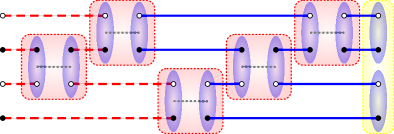
Loop updates. The loop updates SandvikEvertz can be applied here with a slight modification, where loops passing through the Néel state cannot be flipped as in the double projection scheme SandvikEvertz . This can be understood in two different ways: First, in the original scheme loop flips correspond to a flip of underlying spin configurations. Whereas every valence bond and every singlet projector contains two such configurations, the Néel state is a single spin configuration. Therefore, loops through the Néel state exist only in one flavor and cannot be flipped, in contrast to all other loops that exist in two flavors.

Another way of seeing this is by looking at the interpretation of Sutherland’s overlap rule Sutherland described in Fig. 2, which deals only with closed loops but not with open ones. The loop algorithm aims precisely to mimic the varying contributions from the number of loops, by rewriting the term $2^{N_{\bigcirc}}$ as a sum over different configurations. Allowing each closed loop to take two different flavors generates exactly the required sum, whose stochastic sampling is computationally cheaper than counting the number of closed loops in a given overlap graph.

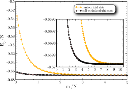
As a result, we keep the flavor of the red (dashed) loops in Fig. 2 constant, while we flip every blue (continuous) loop with a probability of $50\%$ between the two flavors. As in the original scheme SandvikEvertz , the different flavors represent a constraint for all other updates, which can be carried out in completely the same manner as in the original work. This includes operator updates, which are used to move the bond operators into different positions of the overlap graph, as well as state updates, in order to sample the different valence bond states $\left|\varphi_{i}\right>$. Self-optimized amplitude product states SandvikBeach turn out to be an advantageous choice for the single projection scheme as well, as can be seen in Fig. 3. We observe the same benefit for quantities such as Eq. (II). The probabilities of both such updates remain the same as for the double projection scheme SandvikEvertz .

Figure 3: (Color online) Convergence of the ground state energy of a 2D square lattice system with $N=16^{2}$ sites versus the projection length $m$ in a single projection scheme. Inset is a zoom on the low-energy part. For the self-optimized amplitude product state a significant convergence speed up is achieved (error bars are smaller than the point sizes).

Measurements. As the sampling weight $W_{r,i}^{(m)}$ is simply given by

$$W_{r,i}^{(m)}=\frac{a_{i}\left<\mbox{{N\'{e}el}}\right|{P}_{r}^{(m)}\left|\varphi_{i}\right>}{\sum_{r,i}a_{i}\left<\mbox{{N\'{e}el}}\right|{P}_{r}^{(m)}\left|\varphi_{i}\right>}\sim a_{i},$$ (22)

where the remaining factors keep constant during the simulation, the estimator is given by

$$O_{r,i}^{(m)}=\frac{\left<\mbox{{N\'{e}el}}\right|{\cal O}{P}_{r}^{(m)}\left|\varphi_{i}\right>}{\left<\mbox{{N\'{e}el}}\right|{P}_{r}^{(m)}\left|\varphi_{i}\right>}.$$ (23)

Notice that the evaluation of this last expression is very simple, since the denominator is a constant and cancels most of the terms in the numerator. At the end one only has to determine the projected valence bond state ${P}_{r}^{(m)}\left|\varphi_{i}\right>$, which can directly be read out of the overlap graph (Fig. 2) in the following way: Two sites form a valence bond in ${P}_{r}^{(m)}\left|\varphi_{i}\right>$ if they are linked together by an open loop in Fig. 2. Graphically, one just needs to start from any initial site on the Néel state side and follow the open loop until it reaches a second site on the Néel state : The initial and second sites are then coupled in a valence bond in ${P}_{r}^{(m)}\left|\varphi_{i}\right>$. The operator ${\cal O}$ has then to be inserted between this resulting valence bond state and the Néel state itself.

III.3 Application to valence bond occupations and correlations

In the case of valence bond occupations and valence bond correlations the operator ${\cal O}$ is replaced by $-S_{k}^{+}S_{l}^{-}$, which amounts to measure $1$, if the projected valence bond state ${P}_{r}^{(m)}\left|\varphi_{i}\right>$ contains a valence bond $(k,l)$, and $0$ if not. In practice, we measure a histogram of all valence bonds in ${P}_{r}^{(m)}\left|\varphi_{i}\right>$, where we record the length $(x,y)$ of the valence bonds in case of valence bond occupations, or their lengths together with their separation distance in case of valence bond correlations.

Whereas in one dimension it is possible to collect all data for every single valence bond, in higher dimensions we will restrict ourselves to measuring only specific configurations, as the amount of data would otherwise not be manageable.

IV Asymptotic behavior of VB occupation numbers in $d\geq 2$

IV.1 Boundary field theory approach

Let us consider the statistics of VB occupations Eq. (II), in a field theory framework. We note that, when $|\Psi\rangle$ is a ground state, the average VB occupation number between sites $k$ and $l$ [Eq. (9)] for example is given as

$$\bar{n}_{(k,l)}(\left|\Psi\right>)=\lim_{\tau\rightarrow\infty}-\frac{\langle\mbox{{N\'{e}el}}|S^{-}_{k}S^{+}_{l}e^{-\tau{\cal H}}|\Psi_{\rm in}\rangle}{\langle\mbox{{N\'{e}el}}|e^{-\tau{\cal H}}|\Psi_{\rm in}\rangle},$$ (24)

where $|\Psi_{\rm in}\rangle$ is the initial state, which is arbitrary as long as the overlap $\langle\Psi|\Psi_{\rm in}\rangle$ does not vanish. This can be interpreted as a correlation function $\langle S^{-}_{i}S^{+}_{j}\rangle$, in the presence of a boundary described by the “boundary state” $|\mbox{{N\'{e}el}}\rangle$ YellowPages ; BlumenhagenPlauschinn . The boundary condition in the field theory, which exactly matches the Néel state $|\mbox{{N\'{e}el}}\rangle$ as the boundary state, is unknown.

Nevertheless, the large-distance asymptotic behavior of boundary correlation functions is governed by fixed points of boundary renormalization group flow. Those boundary fixed points correspond to conformally invariant boundary conditions. Thus, as long as we are concerned with the large-distance asymptotic behavior of the VB distribution, we can replace the boundary condition with the conformally invariant one corresponding to the infrared fixed point for the boundary RG flow starting from $|\mbox{{N\'{e}el}}\rangle$. In general, tracking the boundary RG flow is a difficult problem. However, in the circumstances we will consider, we can find a natural candidate for such a boundary condition. This approach is generally applicable to the evaluation of the amplitude (inner product) between a reference state and the groundstate of a quantum many-body system in any dimension, at least in principle. We note that this approach indeed has been employed JacobsenSaleur ; StephanMisguichPasquier in $d=1$ dimension, for problems closely related to (but somewhat different from) the present one. Here we demonstrate that it is also useful in $d\geq 2$, and we will come back to $d=1$ in Sec. V.1.

The low-energy/large-distance effective theory of the Heisenberg antiferromagnet on the hypercubic lattice in $d\geq 2$ dimensions is the O(3) nonlinear $\sigma$ model. It is defined by the Lagrangian density

$${\cal L}=\frac{1}{2g}[\partial_{\mu}\vec{m}(\mathbf{r},\tau)]^{2},$$ (25)

where $\vec{m}$ is a three-dimensional vector subject to the constraint

$$\vec{m}^{2}=1.$$ (26)

The field $\vec{m}$ describes the staggered component of the original spin operator:

$$\vec{S}_{\mathbf{r}}\sim(-1)^{s(\mathbf{r})}S\vec{m}(\mathbf{r})+\cdots.$$ (27)

As we have discussed, the ground state of the Heisenberg antiferromagnet in a $d\geq 2$ hypercubic lattice generally displays a long-range antiferromagnetic order. This also implies the spontaneous breaking of the O(3) symmetry in the corresponding non-linear $\sigma$ model, and the field $\vec{m}$ is aligned to a particular direction. Without losing generality, let us assume that $\vec{m}$ is aligned in the $z$ direction. The small fluctuation around the “vacuum” can be described by the two components $m^{x}$ and $m^{y}$, so that

$$m^{z}=\sqrt{1-(m^{x})^{2}-(m^{y})^{2}}.$$ (28)

The Lagrangian density Eq. (25) is now written as

$${\cal L}\sim\frac{1}{2g}\left[(\partial_{\mu}m^{x})^{2}+(\partial_{\mu}m^{y})^{2}\right],$$ (29)

where higher-order terms in $m^{x}$ and $m^{y}$ which come from the expansion of Eq. (28) are neglected. Physically, Eq. (29) represents the theory of two Nambu-Goldstone modes which arise due to the spontaneous symmetry breaking. The ignored higher-order terms correspond to interaction between Nambu-Goldstone bosons. In the present case ($d\geq 2$ and $T=0$), the interactions are irrelevant and the theory of free Nambu-Goldstone bosons (29) is asymptotically exact in the large-distance limit, in the symmetry-broken phase.

While, in general, the direction of ordering in the reference Néel state can be arbitrary in Eq. (24), in the present case we have to choose the reference Néel state with the same ordering direction as in the ground state $|\Psi\rangle$. Otherwise, the overlap would vanish. Thus, here we take the reference Néel state with the ordering in the $z$ direction and use Eq. (24).

In terms of the free Nambu-Goldstone boson field theory Eq. (29), Eq. (24) is proportional to

$$\langle\mbox{{N\'{e}el}}_{z}|m^{x}(0)m^{x}(\mathbf{r})|\Psi\rangle$$ (30)

(a similar term with $m^{y}$ gives the same contribution) note1 . In the Néel state, the spins are completely aligned antiferromagnetically along the $z$ axis. Considering Eq. (27), it is natural to expect that (the infrared limit of) the boundary condition corresponding to $|\mbox{{N\'{e}el}}_{z}\rangle$ is the Dirichlet boundary condition for $m^{x}$ and $m^{y}$:

$$m^{x}(\mathbf{r},0)=m^{y}(\mathbf{r},0)=0,$$ (31)

imposing $\vec{m}=(0,0,1)$, which corresponds to the perfect Néel order in the $z$ direction, at the boundary $\tau=0$.

Thus the valence bond occupation number, in the large-distance limit, is proportional to the correlation function $\langle m^{x}m^{x}\rangle$ along the boundary with the Dirichlet boundary condition. This correlation function appears to vanish, because $m^{x}$ is set to zero on the boundary. However, in adopting the boundary picture in the continuum limit, the operator $m^{x}$ does not have to be exactly at the boundary; generally we expect that they would be rather located within a short distance $\epsilon$, of the order of the ultraviolet cutoff, from the boundary. Namely, we postulate that

$$\bar{n}_{\mathbf{0}\mathbf{r}}\propto\langle m^{x}(\mathbf{0},-\epsilon)m^{x}(\mathbf{r},-\epsilon)\rangle_{D},$$ (32)

where $\langle\cdot\rangle_{D}$ is the expectation value in the presence of the boundary at $\tau=0$, where the Dirichlet boundary condition Eq. (31) is imposed. A similar trick, known as “point-splitting technique” is often used in applications of field theory.

Within the free Nambu-Goldstone boson theory Eq. (29), correlation functions with the Dirichlet boundary condition can be conveniently calculated by the method of mirror images. For example, Eq. (32) can be written as

$$\bar{n}_{\mathbf{0}\mathbf{r}} \propto\langle m^{x}(\mathbf{0},-\epsilon)m^{x}(\mathbf{r},-\epsilon)\rangle_{D}$$

$$=\langle\left[m^{x}(\mathbf{0},\epsilon)-m^{x}(\mathbf{0},-\epsilon)\right]\left[m^{x}(\mathbf{r},\epsilon)-m^{x}(\mathbf{r},-\epsilon)\right]\rangle,$$ (33)

in terms of the correlation functions denoted by $\langle\cdots\rangle$ in the infinite plane. For a small $\epsilon$, it can be expanded as

$$\bar{n}_{\mathbf{0}\mathbf{r}} \propto 4\epsilon^{2}\frac{\partial}{\partial\tau}\frac{\partial}{\partial\tau^{\prime}}\langle m^{x}(\mathbf{0},\tau)m^{x}(\mathbf{r},\tau^{\prime})\rangle\big{|}_{\tau=\tau^{\prime}=0}$$

$$={\rm const.}\frac{\partial}{\partial\tau}\frac{\partial}{\partial\tau^{\prime}}\frac{1}{\left[\mathbf{r}^{2}+(\tau-\tau^{\prime})^{2}\right]^{\frac{d-1}{2}}}\big{|}_{\tau=\tau^{\prime}=0}$$

$$={\rm const.}\frac{1}{|\mathbf{r}|^{d+1}}.$$ (34)

Thus we have derived the power law length distribution of VBs, in agreement with several earlier works Wegner ; Beach ; BeachMaster . The present approach clarifies universality and asymptotic exactness of this power law in quantum Heisenberg antiferromagnets. Moreover, it enables us to discuss correlations among VBs by analyzing the simultaneous occupation number of multiple VBs. As the simplest among such cases, let us discuss the simultaneous occupation number of two VBs as introduced in Eq. (13), and whether there is any correlation between two VBs. Eq. (13) can be written in terms of a four-point correlation function of $m^{x}$ and $m^{y}$, through Eq. (27). Within the free Nambu-Goldsone boson theory Eq. (29), thanks to Wick’s theorem, the four-point correlation function is given in terms of products of two-point correlation functions. We thus find

$$\bar{n}_{\{k_{1},k_{2}\},\{l_{1},l_{2}\}} =\langle m^{x}_{k_{1}}m^{x}_{l_{1}}\rangle\langle m^{x}_{k_{2}}m^{x}_{l_{2}}\rangle$$

$$\phantom{\langle m^{x}_{k_{1}}m^{x}_{l_{1}}\rangle\langle m^{x}_{k_{2}}m^{x}_{l_{2}}\rangle}+\langle m^{x}_{k_{1}}m^{x}_{l_{2}}\rangle\langle m^{x}_{k_{2}}m^{x}_{l_{1}}\rangle$$

$$=\bar{n}_{(k_{1},l_{1})}\bar{n}_{(k_{2},l_{2})}+\bar{n}_{(k_{1},l_{2})}\bar{n}_{(k_{2},l_{1})}$$

$$\propto\frac{1}{{r_{11}}^{d+1}}\frac{1}{{r_{22}}^{d+1}}+\frac{1}{{r_{12}}^{d+1}}\frac{1}{{r_{21}}^{d+1}},$$ (35)

where $r_{mn}$ is the distance between sites $k_{m}$ and $l_{n}$. Namely, it is given simply by a sum of products of the average occupation numbers of the individual VBs. This implies that there is in fact no correlation in valence bond occupations between different pairs of sites, and occupation of each pair occurs independently. This conclusion extends straightforwardly to correlations among occupations of an arbitrary number of bonds. It should be noted that the present field theory describes the asymptotic behavior only in the large-distance limit. The above result does not exclude correlations in a quantum antiferromagnet at short length scales.

IV.2 $d=2$ QMC results

Figure 4: (Color online) Length distribution $P(r)$ of valence bonds of length $r=\sqrt{x^{2}+y^{2}}$ (in all orientations) on different clusters with $N=L^{2}$ sites. The dashed blue line is a guide to the eyes, showing the expected $r^{-3}$ behavior from field theory. This scaling is observed as long as valence bonds are significantly shorter than the finite-size lattice sample. For very long valence bonds, the data exhibit a small upturn above this power law, as well as a slight anisotropy, due to the periodic boundary conditions. Data have been produced for a projection length of $m/N=16$ for all clusters except the biggest one, for which a projection length of $m/N=32$ was chosen (convergence was checked). Error bars are smaller than the point sizes. Inset: Valence bond distribution $\log P(\log(r)\cos\theta,\log(r)\sin\theta)$ in logarithmic polar coordinates with logarithmic color scheme for $N=128^{2}$ in the region $[-L/2,L/2]^{2}$. The data grid is illustrated by small black circles in the range $[-L/4,L/4]^{2}$, whereas the colored mesh represents interpolated data. Outside this range the data grid is very dense and is therefore omitted. For short valence bonds the distribution appears to be rather isotropic, in agreement with the principal figure, whereas the boundary effects of the finite size sample can be observed for very long valence bonds.

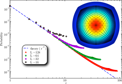
Here we present the numerical results on the VB distribution for the $S=1/2$ Heisenberg antiferromagnet on a $d=2$ square lattice. One first issue to check is whether the distribution of valence bonds with length $(x,y)$ is isotropic, as suggested by the field theory predictions. This can be carried out by simulating different two-dimensional clusters with periodic boundary conditions. Here, we study clusters with $N=16^{2}$, $N=32^{2}$, $N=64^{2}$ and $N=128^{2}$ and provide an example of the distribution $P(x,y)$ of valence bonds with length $(x,y)$ for the biggest cluster in the inset of Fig. 4. Since we expect a power-law decay in $r=\sqrt{x^{2}+y^{2}}$, we choose logarithmic polar coordinates for the $x$-$y$ plane and a logarithmic color scheme for the probability $P(x,y)$. In the figure we see that the distribution seems indeed to be rather isotropic in the center, a behavior that is perturbed for large $r$, due to the periodic boundary conditions.

The isotropic behavior can also be observed in the main panel of Fig. 4, which shows the decay of the probability for measuring a valence bond with length $r$. We observe that almost all points lie on the power law $r^{-3}$ as predicted by the theory Eq. (34).

For very long valence bonds we can see the effect of the boundary as a deviation from the power-law, as well as through a very small anisotropy, characterized by a small spreading fan at large $r$. The points on the envelope of this fan can be identified very accurately. Whereas the upper envelope contains points of valence bonds with lengths $(0,y)$ and $(x,0)$, the bottom envelope describes valence bonds of lengths $(x,x\pm 1)$. Note, that there are no bipartite valence bonds of lengths $(x,x)$.

Another important issue is that the raw data for sufficiently small $r$ in Fig. 4 fall precisely on the same curve for all system sizes, without any extra renormalization. Considering the original definition of the VB distribution $P(r)$, there is no obvious reason why $P(r)$ is independent of the system size. This, however, can be understood rather naturally from the field theory description discussed in Sec. IV.1. Once the VB occupation number is mapped to a correlation function, the latter does not depend on the system size as long as the distance $r$ is much smaller than the system size $L$. In the present problem, the correlation function is not of a standard type, but in the scaling limit it is nonetheless mapped to the boundary correlation function in the field theory. Thus it should not depend on the system size, assuming that the point-splitting scale $\epsilon$ is insensitive to $L$. The mapping to the field theory works only for a sufficiently large $r$. Nevertheless, the system-size independence of the VB distribution $P(r)$ at the shortest distance $r=1$ can be understood even without the field theory mapping. That is, $P(1)$ is related exactly to the ground state energy $E_{0}$ of the underlying Hamiltonian Eq. (1) as

$$\frac{E_{0}}{NJ}=-\frac{1}{4}\left[P(1)+d\right].$$ (36)

Since the ground state energy per site, $E_{0}/N$, is an intensive quantity, so is $P(1)$. It is also natural to expect that $P(r)$ for an arbitrary distance $r$ is also intensive, which is indeed seen in the numerical results.

The sum rule Eq. (11) requires a constraint on the asymptotic power-law behavior $P(r)\sim{\cal C}r^{-\alpha}$ at large distances, which follows from the field theory. Let us assume that the power law is valid for $r>a$, where $a$ is the ultraviolet “cutoff” scale (usually of the order of the lattice constant) above which the field theory applies. Furthermore, here we assume that the proportionality constant ${\cal C}$ is independent of the system size (length) $L$. We first use the decomposition

$$\sum_{\mathbf{r}}P(\mathbf{r})=\sum_{r=|\mathbf{r}|\leq a}P(\mathbf{r})+\sum_{r=|\mathbf{r}|>a}P(\mathbf{r}),$$ (37)

where both terms in the right-hand side are non-negative by definition. In a finite-size system, $r$ is actually cut off by $L$. Thus the second term, which is the large-distance part, is estimated as

$$\sum_{\frac{a}{L}<x=|\mathbf{x}|<1}\frac{{\cal C}}{x^{\alpha}} \sim\frac{{\cal C}}{L^{\alpha-d}}\int_{\frac{a}{L}<x<1}\frac{1}{x^{\alpha}}\;d^{d}\mathbf{x}$$

$$\sim\frac{2\pi^{(d+1)/2}}{\Gamma(\frac{d+1}{2})}\frac{1}{\alpha-d}\frac{{\cal C}}{a^{\alpha-d}},$$ (38)

where $\mathbf{x}\equiv\mathbf{r}/L$. Only the leading singular part in $L\rightarrow\infty$ is retained in the integral in the last manipulation, which is valid only if $\alpha>d$. This shows that the total contribution from the large-distance part of $P(\mathbf{r})$ is finite even in the thermodynamic limit $L\rightarrow\infty$ and thus the sum rule Eq. (11) can be satisfied. If $\alpha\leq d$, on the other hand, the contribution from the large-distance part is divergent and consequently the sum rule will be violated. Therefore, the sum rule Eq. (11) requires that the asymptotic large-distance power law should have either $\alpha>d$ or the proportionality constant ${\cal C}$ depending on the system size $L$. Our finding that $\alpha=d+1$ and ${\cal C}$ is system-size independent is consistent with this constraint.

Figure 5: (Color online) a) Choice of the swapped regions ${\cal S}_{A}$ and ${\cal S}_{B}$ in order to measure the correlation between two valence bonds (shaded ellipses) of lengths $r$, drawing an angle of $\alpha=\pi/2$. Notice that Eq. (II) yields one when two valence bonds connect ${\cal S}_{A}$ and ${\cal S}_{B}$ and vanishes otherwise. This is true for the illustrated VB configuration, as well as for the one that is sketched by the dashed lines. b) The same configuration with two valence bonds drawing an angle of $\alpha=0$.

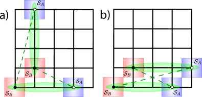
Second, we want to study VB-VB correlations in the ground state of the Heisenberg antiferromagnet. In order to see whether correlations are present in two dimensions we choose the two cases that are depicted in Fig. 5, since we intuitively expect correlations to be most pronounced when two valence bonds are very close to each other. We refer to these two cases as those where two valence bonds of equal length draw an angle of a) $\alpha=\pi/2$ and b) $\alpha=0$. We shall here emphasize again that we cannot directly measure the simultaneous occupation number of two VBs for specified pairs of the sites, but only the sum of occupation numbers corresponding to two possible VB patterns. In the present case, these patterns are drawn as shaded ellipses and dashed lines in Fig. 5, respectively. In the case a) $\alpha=\pi/2$, for example, we have two valence bonds of lengths $(r,0)$ and $(0,r)$ and two other valence bonds of lengths $(r-1,1)$ and $(1,r+1)$. In the case b) we encounter the same valence bond lengths, but at a different angle $\alpha=0$.

Let $C_{\alpha}(r)$ with $\alpha=0,\pi/2$ represent the simultaneous VB occupation numbers in the two cases a) and b), respectively. If there is no correlation between the two VBs, the normalized simultaneous VB occupation number on the pair should be given as

$$C_{\alpha=\pi/2}(r)=C_{\alpha=0}(r)$$

$$=P(r)^{2}+P(\sqrt{r^{2}+2r+2})P(\sqrt{r^{2}-2r+2}),$$ (39)

where we used the isotropy of the single VB occupation number $P({\bf r})=P(r)$ on a given pair of sites separated by ${\bf r}=(x,y)$. In fact, there are no other patterns that are expected to have exactly the same decomposition as in Eq. (39).

In order to verify Eq. (39), we have to find the proper constant of proportionality. Here it is important, that we used translational and rotational invariance in order to measure $P(x,y)$, $C_{\alpha=0}(r)$ and $C_{\alpha=\pi/2}(r)$, accounting for a factor of $N$ in all cases. For this reason it is obvious that the appropriate constant of proportionality must be $1/N$. Therefore, we have to multiply the correlation data by the system size, when comparing different system sizes $L$, since $P(x,y)$ does not depend on $L$. Furthermore, patterns of $C_{\alpha=0}(r)$ appear only half as much as those for $C_{\alpha=\pi/2}(r)$, due to rotational symmetry.

Figure 6: (Color online) Simultaneous occupation number of two VBs on bonds that draw an angle $\alpha$ between them, as illustrated in Fig. 5. For comparison, we also show the sum of the products of corresponding single VB occupation numbers as in the right-hand side of Eq. (39). Data were obtained for clusters of $N=L^{2}$ sites with a projection length of $m/N=16$ (convergence checked) and error bars are smaller than the point sizes. The good agreement among the three different sets of data confirms the decomposition as in Eq. (39), which indicates the asymptotic absence of the correlation between two VBs. This also implies the agreement with the field theory prediction $\propto r^{-6}$, as shown.

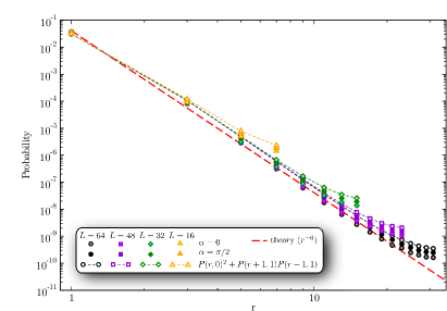
The properly normalized data are plotted in Fig. 6, and show essentially the expected $\sim r^{-6}$ behavior. This power law is also obtained by the simple product of the pure valence bond occupations, which indicates the absence of correlations between VBs in two dimensions. Interestingly, the very first data point for $r=1$ seems to be slightly above the predicted power law $\sim r^{-6}$. In fact, this point is the only one where the correlation data are slightly above the sum of the products of the occupation numbers for the individual VBs. In the entire rest of the range, this is not the case. This implies the existence of a correlation among VBs at very short distances $r\sim 1$. Such an effect seems to be in agreement with some recent results, which conclude that including correlations between valence bonds at very short distances can indeed improve the energy for variational calculations Lin12 . In any case, this does not contradict the field theory analysis, which only applies to the asymptotic behavior at large distances. In fact, the present numerical analysis demonstrates that the field theory works very well above the rather short length scale $r>a\sim\sqrt{2}$.

For larger $r$ comparable to the system size $L$, we see the effects of the periodic boundary conditions, and the data do not follow the field theoretical prediction for the infinite system any more. We furthermore see a more pronounced splitting between the different data for $C_{\alpha=\pi/2}(r)$, $C_{\alpha=0}(r)$ and the valence bond occupation product. However, these differences are very small (of order $10^{-10}$) compared to the correlations between short valence bonds.

IV.3 $d=3$ QMC results

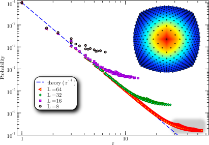
In order to check that the same field theory also applies to higher dimensions, we here present QMC results for the case $d=3$. Because simulations become more and more demanding as we increase the dimension, we restrict ourselves to the distribution of valence bonds $P(r)$, which is depicted in Fig. 7 for samples of up to $N=64^{3}$ sites. Furthermore, for the biggest cluster we could not achieve convergence of the data for $r\gtrsim 25$ (fortunately, this is a region where boundary effects start to play a role and where deviations from field theory predictions are therefore expected).

As expected, we observe the same behavior as in two dimensions, but with the exponent in the power law now being equal to $4$. We furthermore observe that the distribution is still isotropic in three dimensions, as can be seen in the inset of Fig. 7, where a two-dimensional cut through the data is shown.

Figure 7: (Color online) Length distribution $P(r)$ of valence bonds of length $r=\sqrt{x^{2}+y^{2}+z^{2}}$ (in all orientations) on different clusters with $N=L^{3}$ sites. The dashed blue line is a guide to the eyes, showing the expected $r^{-4}$ behavior from field theory. Notice that qualitatively the only difference from the case $d=2$ (Fig. 4) is the exponent in the observed power law, due to the higher dimension. Data have been produced for a projection length of $m/N=4$ for the two smallest lattices and $m/N=8$ for $L=32$ (convergence was checked) and error bars are smaller than the point sizes. For $L=64$ we used a relatively small projection length of $m/N=2$, resulting in non-converged data for $r\gtrsim 25$ (highlighted in gray). Inset: Valence bond distribution $\log P(\log(r)\cos\theta,\log(r)\sin\theta)$ in logarithmic polar coordinates with logarithmic color scheme for $N=32^{3}$ in the region $[-L/2,L/2]^{2}$ within the y-z plane (at $x=0$). The data grid is illustrated by small black circles, whereas the colored mesh represents interpolated data. Similarly as for $d=2$, for short valence bonds the distribution appears to be rather isotropic, in agreement with the main panel, whereas the boundary effects of the finite-size sample can be observed for very long valence bonds.

V Asymptotic behavior of VB occupation numbers and their correlations in $d=1$

V.1 Boundary field theory approach in $d=1$: Bosonization

The physics of the $S=1/2$ Heisenberg antiferromagnet in a $d=1$ chain is quite different from that of the same model in the $d\geq 2$ hypercubic lattice. In $d=1$, quantum fluctuations are so strong that the long-range antiferromagnetic order is absent even in the ground state. The ground state of the $S=1/2$ antiferromagnetic chain is critical: Various correlation functions decay algebraically. The universal behaviors in the low-energy, long-distance regime are described Affleck-LesHouches88 as a Tomonaga-Luttinger liquid (TLL). This is a free-boson field theory defined by the Lagrangian density

$${\cal L}=\frac{1}{2}(\partial_{\mu}\phi)^{2}.$$ (40)

The field $\phi$ obeys the equation of motion, which is nothing but the wave equation in one spatial dimension. As a consequence, $\phi$ can be decomposed as

$$\phi(x,t)=\phi_{R}(x-t)+\phi_{L}(x+t),$$ (41)

where $\phi_{R,L}$ are right-moving and left-moving components. We also introduce the dual field $\tilde{\phi}$, which is defined by

$$\tilde{\phi}=\phi_{R}-\phi_{L}.$$ (42)

The spin operators are represented in terms of the boson field $\phi$ as

$$S^{z}_{j} \sim\frac{1}{2\pi R}\frac{\partial\phi}{\partial x}+{\rm const.}(-1)^{j}\cos{\frac{\phi}{R}},$$ (43)

$$S^{\pm}_{j} \sim{\rm const.}e^{\pm 2\pi Ri\tilde{\phi}}\cos{\frac{\phi}{R}}+{\rm const.}(-1)^{j}e^{\pm 2\pi Ri\tilde{\phi}},$$ (44)

where $R$ is a parameter of the theory called the compactification radius. For the isotropic Heisenberg antiferromagnetic chain,

$$R=\frac{1}{\sqrt{2\pi}}.$$ (45)

Despite the significant difference in physics between $d=1$ and $d\geq 2$, it is possible to construct a boundary field theory formulation of VB distributions in $d=1$ as well. First, let us identify the conformally invariant boundary condition, which would be the infrared fixed point for the given boundary state $|\mbox{{N\'{e}el}}\rangle$. In the reference Néel state, the staggered component of $S^{z}$ is fixed to a constant. Thus it is natural to expect that the Dirichlet boundary condition $\phi=0$ is the appropriate boundary condition. The Dirichlet boundary conditon is in fact conformally invariant. Assuming that this is the case, the valence bond occupation number is just given by the correlation function $\langle S^{+}S^{-}\rangle$ along the boundary, where the Dirichlet boundary condition $\phi=0$ is imposed. This problem is reduced to the correlation function of the vertex operators in the presence of the Dirichlet boundary condition: $\langle e^{2\pi Ri\tilde{\phi}}e^{2\pi Ri\tilde{\phi}}\rangle_{D}$.

Such boundary correlation functions have been studied in great detail in boundary conformal field theory. In the present case with the Dirichlet boundary condition, the calculation can be quite easily done as follows. Let us assume the system is defined on the half plane $\tau<0$ and the boundary is at $\tau=0$, along the $x$ axis.

Because of Eq. (41), imposing the Dirichlet boundary condition $\phi=0$ at the boundary $\tau=0$ is equivalent to extending the chiral field $\phi_{R}$ to the other side of the boundary $\tau>0$, where no field was originally defined, by the following relation:

$$\phi_{R}(x,\tau)=-\phi_{L}(x,-\tau).$$ (46)

This means that the dual field at the boundary $\tau=0$ can be written entirely in terms of the chiral field $\phi_{R}$. Moreover, the correlation function of the chiral field can be evaluated in the infinite plane without boundary. Combining this observation with Eqs. (24) and (44), the large distance asymptotic behavior of the valence bond occupation number is given as

$$\bar{n}_{jk}\propto\langle e^{i4\pi R\phi_{R}}e^{-i4\pi R\phi_{R}}\rangle,$$ (47)

where $\langle\cdot\rangle$ now means the expectation value in the infinite plane without a boundary. The result can be readily obtained as

$$\langle e^{i4\pi R\phi_{R}}e^{-i4\pi R\phi_{R}}\rangle ={\rm const.}\frac{1}{r^{4\pi R^{2}}}$$ (48)

$$={\rm const.}\frac{1}{r^{2}},$$ (49)

where $r$ is the distance between the two sites $j$ and $k$, and we have set $R=1/\sqrt{2\pi}$ for the isotropic Heisenberg chain in the second line. Despite the difference in the formulation, the final result for the single VB occupation number in $d$ dimensions can be summarized as $1/r^{d+1}$, whether $d=1$ or $d\geq 2$.

On the other hand, correlations among VBs reveal an interesting difference between $d=1$ and $d\geq 2$. Although the effective field theory (TLL) is also a free-boson field theory, (the staggered part of) the spin operator is expressed by a vertex operator (exponential in the boson field), and not by the boson field itself. Thus, while Wick’s theorem certainly applies to the TLL, it does not mean the absence of correlations in multipoint correlation functions of spins, and consequently, among the VB occupations.

In fact, the simultaneous occupation number of two VBs [Eq. (13)] can be evaluated exactly within the TLL theory formulation Eq. (40). Following the same logic as in the single VB occupation number, we find

$$\bar{n}_{\{x_{1},x_{2}\},\{x^{\prime}_{1},x^{\prime}_{2}\}}$$

$$\propto\langle e^{4\pi Ri\phi_{R}(x_{1})}e^{4\pi Ri\phi_{R}(x_{2})}e^{-4\pi Ri\phi_{R}(x^{\prime}_{1})}e^{-4\pi Ri\phi_{R}(x^{\prime}_{2})}\rangle$$

$$\propto\left(\frac{r_{A}r_{B}}{r_{11}r_{22}r_{12}r_{21}}\right)^{2},$$ (50)

where $x_{1},x_{2}\in A$, $x^{\prime}_{1},x^{\prime}_{2}\in B$, and

$$r_{mn} =|x_{m}-x^{\prime}_{n}|,$$ (51)

$$r_{A} =|x_{1}-x_{2}|,$$ (52)

$$r_{B} =|x^{\prime}_{1}-x^{\prime}_{2}|.$$ (53)

Again we have assumed $R=1/\sqrt{2\pi}$ for the SU(2) symmetric Heisenberg antiferromagnetic chain.

When two bonds are separated by a large distance (relative to the bond lengths), namely, in the limit

$$r_{A}\sim r_{B}\sim r_{12}\sim r_{21}\gg r_{11}\sim r_{22},$$ (54)

we find

$$\bar{n}_{\{x_{1},x_{2}\},\{x^{\prime}_{1},x^{\prime}_{2}\}}\sim\left(\frac{1}{r_{11}r_{22}}\right)^{2}.$$ (55)

This implies that

$$\bar{n}_{\{x_{1},x_{2}\},\{x^{\prime}_{1},x^{\prime}_{2}\}}\sim\overline{n_{(x_{1},x_{2})}}.\overline{n_{(x^{\prime}_{1},x^{\prime}_{2})}}.$$ (56)

Namely, the correlation asymptotically vanishes, as the separation between two VBs is taken to infinity. This is consistent with our intuitive expectation.

On the other hand, for general separation, our result exhibits a nontrivial correlation between VB occupation. A major feature of the correlation is that, because of the factor $r_{A}r_{B}$ in the numerator, the simultaneous occupation amplitude vanishes as $x_{1}\rightarrow x_{2}$ or $x_{1}^{\prime}\rightarrow x_{2}^{\prime}$.

V.2 $d=1$ QMC results

Figure 8: (Color online) Length distribution $P(r)$ of valence bonds as a function of $r$ for one-dimensional lattices with $L$ sites as obtained from QMC calculations, versus field theory predictions. All chains were simulated for a projection length of $m/L=64$ and the convergence was checked (error bars are smaller than the point sizes). Note that we applied the conformal transformation $r=L/\pi\sin(\pi x/L)$, where $x$ is the measured valence bond length.

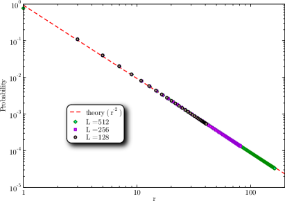
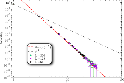
Let us now compare the theoretical predictions above with the numerical results obtained by QMC simulations. As we have seen earlier, QMC simulations are restricted to finite sizes, and the VB distribution functions inevitably deviate from the theoretical predictions which were made for an infinite system. Fortunately, however, our theory for $d=1$ is based on the TLL, which is a conformal field theory in $1+1$ dimensions. In this class of field theory, the finite-size effect is conveniently described by a conformal mapping YellowPages . The rule of thumb is that, in order to obtain a correlation function in a finite system (ring) of length $L$ with the periodic boundary condition, a distance $r$ appearing in the corresponding correlation function in the infinite system should be replaced by the arc distance $r=(L/\pi)\sin{(\pi x/L)}$ on the finite ring. In the one-dimensional case we also first check the length distribution $P(r)=\bar{n}_{k,l}$ of the valence bonds, as plotted in Fig. 8. The simulations are carried out on the one-dimensional Heisenberg chain with $L=128$, $256$ and $512$ sites and periodic boundary conditions. We find a power-law decay $P(r)\sim{\cal C}r^{-2}$, which agrees very well with the field theory prediction Eq. (49) with the conformal mapping.

Here again, all the data in Fig. 8 for different system sizes appear to collapse on a single curve, without any rescaling. That is, the normalization constant ${\cal C}$ is independent of the system size. As we have discussed in Sec. IV.2, this can be naturally understood from the mapping to the boundary correlation function and the intensiveness of the ground state energy per site. In fact, we can make the analysis in Eq. (11) more precise, by using the correlation function in a finite system of length $L$ obtained by the conformal mapping, as

$${\cal C}\sum_{\frac{a}{L}<x=|\mathbf{x}|<1}\left(\frac{1}{L\sin{(\pi x)}}\right)^{\alpha} \sim\frac{{\cal C}}{L^{\alpha-1}}\int_{\frac{a}{L}<x<1}\left(\frac{1}{\sin{\pi x}}\right)^{\alpha}\;dx$$

$$\sim\frac{2}{\alpha-1}\frac{{\cal C}}{a^{\alpha-d}}.$$ (57)

The leading contribution in the limit of $L\rightarrow\infty$, for $\alpha>1$, however remains the same as in Eq. (11) with $d=1$. For $\alpha<1$, the large-distance contribution diverges, as in the case of $\alpha<d$ for general dimension $d$. Our finding that ${\cal C}$ is independent of the system size and that $\alpha=d+1$ applies also to $d=1$, again in consistency with the sum rule Eq. (11).

Only at the shortest distance $r=1$, there is a visible difference between the numerical result and the field theory prediction. As in $d\geq 2$, the disagreement between the data and the field theory prediction is not surprising, as the field theory describes only the long-distance asymptotic behaviors. The data imply that the ultraviolet cutoff scale $a$, above which the field theory is valid, is small ($\sim 1$) also in $d=1$.

Figure 9: (Color online) a) Choice of the disconnected swapped regions ${\cal S}_{A}$ (separated by $r_{A}=2$) and ${\cal S}_{B}$ (separated by $r_{B}=2$) with the corresponding valence bonds of lengths $r_{11}$ and $r_{22}$. b) There is also another possible configuration of bipartite valence bonds with lengths $r_{12}$ and $r_{21}$.

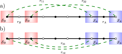
We now study the correlations between VBs on the Heisenberg chain, where we choose again the case of two equally long close valence bonds, as illustrated in Fig. 9. Again, there are two possible VB patterns and we choose $x=r_{11}$ as the varying parameter. The results are plotted in Fig. 10. Notice first of all, that Eq. (53) uses conformal coordinates, such that we expect a power-law decay as $\sim r^{-8}\propto\sin^{-8}(\pi x/L)$ for sufficiently long valence bonds. This implies, however, a rather drastic decrease of probabilities, resulting in relatively rare events. This is indeed observed in the simulations, where probabilities of $10^{-11}$ with pronounced error bars are encountered. Nevertheless, we can confirm the predicted $\sim r^{-8}$ behavior and clearly exclude a possible $\sim r^{-4}$ power-law decay obtained from a simple product of valence bond occupations $C_{\rm No\quad\!\!\!\!\!corr}(x)=P(x)^{2}+P(x-2)\cdot P(x+2)$. This is a strong indication, that correlations are indeed present even at large distances, in one dimension.

Figure 10: (Color online) Correlations between valence bonds (in the configuration of Fig. 9) in the ground state of Eq. (1) on $1D$ chains of different sizes $L$. The measured correlations multiplied by system size (data points) clearly agree with the field theory predictions of a power-law decay $r^{-8}$ (red dashed curve). All data were obtained with projection lengths of $m/L=64$ (convergence was checked) and the error bars are smaller than the point sizes if omitted. Notice, that we applied the conformal transformation $r=L/\pi\sin(\pi x/L)$, with $x$ being the measured distances.

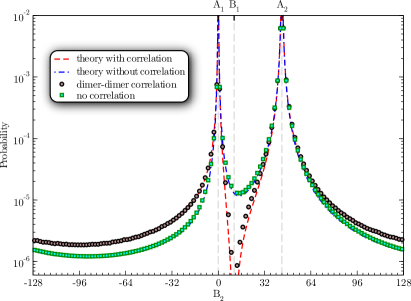
In order to further examine this behavior, we now study a case where three points of this four-point correlation function are fixed and one point is variable, as shown in Fig. 11. We plot the VB-VB correlations, as well as the product of the valence bond occupations, which both reproduce the theoretical predictions. In agreement with our naive intuition, both theories show the same behavior if we consider short valence bonds, separated by a rather large distance. This can be seen in the figure when $x\approx A_{1}$ or $x\approx A_{2}$ and means that no further correlations are present in such a case. However, the two curves differ considerably for $x\approx B_{1}$, i.e., when the two valence bonds start affecting each other. This confirms that in such a case correlation effects are clearly important in one dimension.

Figure 11: (Color online) VB-VB correlations on a chain with $L=256$ sites for the two (undistinguishable) configurations $\left|(A_{1},B_{1})(A_{2},B_{2})\right>$ and $\left|(A_{1},B_{2})(A_{2},B_{1})\right>$, with $A_{1}=0$, $A_{2}=44$, $B_{1}=11$ and $B_{2}=x$ varying. We show the product of valence bond occupations (green squares), that fit to a theory without correlation as comparison. However, the measured correlations (multiplied by the system sizes, shown as black circles) rather correspond to a theory with correlations. Notice, how the two theories agree asymptotically around $A_{1}$ and $A_{2}$ and disagree substantially at $B_{1}$. The projection length is $m/L=64$ (convergence was checked) and error bars are smaller than point sizes.

VI Discussion and conclusion

Through a combination of analytical calculations and quantum Monte Carlo simulations, we have investigated the behavior of valence bond probability distributions and correlations in ground states of the antiferromagnetic Heisenberg model on chain, square and cubic lattices.

Our analytic results provide a clear ground for the probability distribution $P({\bf r})$ for a valence bond to join two sites (existing on different sublattices) separated by $\mathbf{r}$ to scale as $|\mathbf{r}|^{-(d+1)}$ where $d$ is the lattice dimension. This result, which was observed in previous numerical simulations and justified by a mean-field ansatz, is now understood within a more trustworthy analytical framework: bosonisation in 1D, and the non-linear $\sigma$ model in $d>1$. This will be useful for variational calculations, or for constructing guiding wave functions in Monte Carlo simulations, which aim at targeting an antiferromagnetic state on a bipartite lattice.

Moreover, our results provide a formal justification for the factorization ansatz Eq. (2) introduced by Liang, Douçot and Anderson, as long as a non-linear $\sigma$ model description is valid. Indeed, our results, corroborated by large-scale QMC calculations in the 2D case, clearly indicate the absence of correlations between valence bonds at long distances. For the quasi-long-range ordered ground state of the Heisenberg chain, the situation is more subtle as correlations are present between valence bonds, as clearly observed in Fig. 11. This may be understood as a signature of the strong (power-law-decaying) dimer correlations which are known Giamarchi to be present in the Heisenberg AF chain.

We would also like to point out that the existence of long-range antiferromagnetic order does not necessarily imply a distribution of valence bonds with a distribution law $P({\bf r})\propto|{\bf r}|^{-(d+1)}$ with no correlations. For instance, the wave functions composed of the equal-weight linear combinations of nearest-neighbor valence bonds on the simple cubic or diamond lattices have been shown to sustain AF long-range order Albuquerque12 (see also Ref. Xu13, ). However, their description is most certainly beyond the non-linear $\sigma$ model approach, which probably cannot describe the dipolar dimer correlations observed in these wave functions Albuquerque12 .

Finally, we suggest several further investigations as possible extensions of our work. For one-dimensional systems, the bosonization analysis of Sec. V.1 carries over for the critical phase of the $XXZ$ anisotropic spin chain. While the SU(2) symmetry is lost in this more general case, analytical predictions for mixed expectation values of the type $\langle\mbox{N\'{e}el}|S^{+}_{i}S^{-}_{j}S^{+}_{k}S^{-}_{l}|\Psi\rangle$ [such as in Eq. (II)] can be made and tested through, for instance, DMRG or QMC calculations. In general, the power-law exponent will depend on the anisotropy parameter through the compactification radius $R$. Another interesting problem would be to calculate analytically logarithmic corrections to the power-law decays of valence bond occupations and correlations in one dimension, which most certainly exist in the SU($2$) case. We note, however, that these are presumably small, hard to detect, effects as the QMC results are already very well described by the pure power-law decays.

In dimensions larger than 1, the non-linear $\sigma$ model approach may also be used to describe the behavior of valence bond distributions and correlations at a quantum critical point between the antiferromagnet and a paramagnet, such as for a bilayer Heisenberg model SandvikScalapino ; SandvikChubukov . This could be useful in explaining and improving variational approaches based on valence bonds that aim to describe this quantum phase transition (such as, e.g., Ref. Liao, ). More generally, the current formalism based on the overlap Eq. (II) could be used with any effective field theory which describes a particular quantum phase or a quantum critical point of quantum antiferromagnets on bipartite lattices.

Finally, it would be very interesting to see whether an approach similar to the one developed here could be applied to describe the “spinon detection” procedure recently advocated by Tang and Sandvik Tang , which is also based on a valence bond description of a spin system with one or two unpaired spins (i.e., that do not belong to a valence bond). This is a more challenging case as one would first need to derive equations similar to Eq. (7) or (II) for this situation.

References

- (1) H. Bethe, Z. Phys. 71, 205 (1931); N.D. Mermin and H. Wagner, Phys. Rev. Lett. 17, 1133 (1966)
- (2) E. Jordão Neves and J. Fernando Peres, Phys. Lett. A 114, 331 (1986); I. Affleck, T. Kennedy, E.H. Lieb and H. Tasaki, Commun. Math. Phys. 115, 477 (1988); F.J. Dyson, E.H. Lieb and B. Simon, J. Stat. Phys. 18, 335 (1978)
- (3) M.S. Makivić and H.-Q. Ding, Phys. Rev. B 43, 3562 (1991)
- (4) A.W. Sandvik and H.-G. Evertz, Phys. Rev. B. 82, 024407 (2010).
- (5) E. H. Lieb and D. C. Mattis, J. Math. Phys. 3, 749 (1962).
- (6) G. Rumer, E. Teller and H. Weyl, Nachr. Ges. Wiss. Goettingen, MathPhys. Kl. 499 (1932); L. Hulthén, Ark. Mat. Astron. Fys. B 26A, 1 (1938).
- (7) P.W. Anderson, Mater. Res. Bull. 8, 153 (1973); P. Fazekas and P.W. Anderson, Philos. Mag. 30, 423 (1974).
- (8) R.R.P. Singh and D.A. Huse, Phys. Rev. Lett. 68, 1766 (1992); B. Bernu et al., Phys. Rev. B 50, 10048 (1994); L. Capriotti, A.E. Trumper, and S. Sorella, Phys. Rev. Lett. 82, 3899 (1999); S.R. White and A.L. Chernyshev, Phys. Rev. Lett. 99, 127004 (2007)
- (9) R. Moessner and S. L. Sondhi, Phys. Rev. Lett. 86, 1881 (2001).
- (10) G. Misguich, D. Serban, and V. Pasquier, Phys. Rev. Lett. 89, 137202 (2002).
- (11) See e.g. M. Mambrini and F. Mila, Eur. Phys. J. B 17, 651 (2000).
- (12) M. Mambrini, A. Läuchli, D. Poilblanc and F. Mila, Phys. Rev. B 74, 144422 (2006)
- (13) J. Lou and A.W. Sandvik, Phys. Rev. B 76, 104432 (2007).
- (14) X. Zhang and K.S.D. Beach, Phys. Rev. B 87, 094420 (2013).
- (15) R. Saito, J. Phys. Soc. Jap. 59, 482 (1990); H.N. Temperley and E.H. Lieb, Proc. Roy. Soc. Lond. A. 322, 251 (1971)
- (16) P.W. Anderson, Basic Notions of Condensed Matter Physics (Benjamin, New York, 1984).
- (17) K.S.D. Beach and A.W. Sandvik, Nucl. Phys. B 750, 142 (2006).
- (18) M. Mambrini, Phys. Rev. B 77, 134430 (2008).
- (19) S. Liang, B. Douçot and P.W. Anderson, Phys. Rev. Lett. 61, 365 (1988)
- (20) A.W. Sandvik, Phys. Rev. Lett. 95, 207203 (2005)
- (21) K.S.D. Beach, Phys. Rev. B 79, 224431 (2009).
- (22) K.S.D. Beach, preprint arXiv:0707.0297 (2007) (unpublished).
- (23) F.J. Wegner, Z. Phys. B 85, 259 (1991).
- (24) Note however that Ref. Beach, demonstrates that the amplitude product state is a correct ansatz for a long-range Heisenberg spin model, treated at the mean-field level.
- (25) F. Alet, I.P. McCulloch, S. Capponi, and M. Mambrini, Phys. Rev. B 82, 094452 (2010)
- (26) P. Di Francesco, P. Mathieu, and D. Sénéchal, Conformal Field Theory, Springer (1997).
- (27) R. Blumenhagen and E. Plauschinn, Introduction to Conformal Field Theory: With Applications to String Theory, Lecture Notes in Physics 779, Springer (2009).
- (28) E. Fradkin and J. E. Moore, Phys. Rev. Lett. 97, 050404 (2006).
- (29) M. Oshikawa, preprint arXiv:1007.3739 (2010) (unpublished).
- (30) J. L. Jacobsen and H. Saleur, Phys. Rev. Lett. 100, 087205 (2008)
- (31) J.-M. Stéphan, G. Misguich, and V. Pasquier, Phys. Rev. B 84, 195128 (2011).
- (32) D.A. Huse and V. Elser, Phys. Rev. Lett. 60, 2531 (1988)
- (33) F Mezzacapo et al., New J. Phys. 11, 083026 (2009) (2009), H.J. Changlani et al., Phys. Rev. B 80, 245116 (2009); S. Al-Assam et al., Phys. Rev. B 84, 205108 (2011)
- (34) Y.-C. Lin, Y. Tang, J. Lou and A.W. Sandvik, Phys. Rev. B 86, 144405 (2012)
- (35) X. Zhang, J. Xu and K. S. D. Beach, preprint arXiv:1310.6030 (2013) (unpublished).
- (36) W. Marshall, Proc. R. Soc. London Ser. A 232, 48 (1955).
- (37) A.W. Sandvik and K.S.D. Beach, in Computer Simulation Studies in Condensed-Matter Physics XX, ed. D. P. Landau, S. P. Lewis, and H.-B. Schüttler (Springer, Berlin, 2008).
- (38) D. Schwandt, F. Alet and S. Capponi, Phys. Rev. Lett. 103, 170501 (2009).
- (39) M. B. Hastings, I. Gonzalez, A. B. Kallin and R.G. Melko, Phys. Rev. Lett. 104, 157201 (2010).
- (40) F. Alet et al., Phys. Rev. Lett. 99, 117204 (2007); R.W. Chhajlany, P. Tomczak, and A. Wójcik, Phys. Rev. Lett. 99, 167204 (2007); A.B. Kallin, I. González, M.B. Hastings, and R.G. Melko Phys. Rev. Lett. 103, 117203 (2009); H. Tran and N.E. Bonesteel, Phys. Rev. B 84, 144420 (2011).
- (41) B. Sutherland, Phys. Rev. B 37, 3786 (1988).
- (42) Following the logic here, exchanging and still gives the same result in the field theory. However, in the original formula Eq. (24), the amplitude vanishes after the exchange of the spin operators and . This shows the presence of a subtlety in the mapping to the field theory. Despite this, we believe that the asymptotic large-distance limit is correctly given by the present field-theory prescription, for the appropriate (nonvanishing) amplitude. This will be also supported by numerical calculations in Sec. IV.2.
- (43) I. Affleck, in Fields, Strings and Critical Phenomena. Proceedings of the Les Houches Summer School 1988, E. Brézin and J. Zinn-Justin (eds.), North Holland (1990).
- (44) T. Giamarchi and H. J. Schulz, Phys. Rev. B 39, 4620 (1989).
- (45) A.F. Albuquerque, F. Alet, and R. Moessner, Phys. Rev. Lett. 109, 147204 (2012)
- (46) J. Xu and K. S. D. Beach, preprint arXiv:1311.0004 (2013) (unpublished).
- (47) A.W. Sandvik and D. J. Scalapino, Phys. Rev. Lett. 72, 2777 (1994)
- (48) A.W. Sandvik, A.V. Chubukov and S. Sachdev, Phys. Rev. B 51, 16483 (1995)
- (49) H. Liao and T. Li, J. Phys.: Condens. Matter 23, 475602 (2011).
- (50) Y. Tang and A.W. Sandvik, Phys. Rev. Lett. 107, 157201 (2011); Phys. Rev. Lett. 110, 217213 (2013).