Clustering Markov Decision Processes For Continual Transfer
Abstract
We present algorithms to effectively represent a set of Markov decision processes (MDPs), whose optimal policies have already been learned, by a smaller source subset for lifelong, policy-reuse-based transfer learning in reinforcement learning. This is necessary when the number of previous tasks is large and the cost of measuring similarity counteracts the benefit of transfer. The source subset forms an ‘-net’ over the original set of MDPs, in the sense that for each previous MDP , there is a source whose optimal policy has regret in . Our contributions are as follows. We present EXP-3-Transfer, a principled policy-reuse algorithm that optimally reuses a given source policy set when learning for a new MDP. We present a framework to cluster the previous MDPs to extract a source subset. The framework consists of (i) a distance over MDPs to measure policy-based similarity between MDPs; (ii) a cost function that uses to measure how good a particular clustering is for generating useful source tasks for EXP-3-Transfer and (iii) a provably convergent algorithm, MHAV, for finding the optimal clustering. We validate our algorithms through experiments in a surveillance domain.
Keywords: Reinforcement learning, transfer learning, Markov decision process, MDP abstractions, policy reuse, Markov chain Monte Carlo, discrete optimisation.
1 Introduction
Reinforcement learning (RL) in Markov decision processes (MDPs) is a well known framework in machine learning for modelling artificial agents (Puterman, 1994; Sutton and Barto, 1998), where the agent’s task is one of sequential decision making. While problems such as policy learning in these MDPs are well posed in terms of an objective such as maximising the expected reward, they are often based on a specific instance of an underlying Markov Decision Process model which may or may not be explicitly known to the learning agent.
Realistic agents must cope with environments with variability, wherein a process generates many instances of MDPs within which the agent must now solve the optimisation problem. Finding optimal policies with respect to an unrestricted family of possible MDPs is not only intractable, but often leads to highly conservative and not practicable solutions. However, many realistic environments actually occupy a middle ground.
In many reinforcement learning problems, that are of great interest in practice, the main source of complexity is partial variability in task description rather than a complete change in the domain. Stated in the language of MDPs, these domains involve a family of possible reward and transition functions over a shared state-action space. This is typically the result of non-stationary behavior of some component that describes the problem. One class of problems is where the human-machine interaction setting remains the same, while the participants change. A recent, highly successful example of such a problem is that of website morphing (Hauser et al., 2009). In this problem, the goal is to present to the user of a website a view/interface adapted to the needs and skill level (savvy, newbie etc.) of that particular user. The interface to present to a user is determined adaptively based on the sequence of her choice of links. So, even though the setting (i.e. the website) remains the same , the dynamics defining the problem (the links the user might choose) changes with each user – i.e. each user corresponds to a new task and corresponding change in problem dynamics. Given the change in dynamics, the algorithm has to determine the best policy/sequence of actions (sequence of interfaces to present). Note that since the algorithm knows that a new user has arrived at the homepage, it always knows if the dynamics may have changed – but not how it has changed. In the MDP formalism, each task corresponds to a particular reward and transition function, while the state and action space remain the same across tasks. Additionally, the reinforcement learning agent is always told when the dynamics/task have changed.
In this paper, we present an approach to dealing with such problems that is based on the notion of transfer learning. We view the new task instance as being similar to previously experienced ones, although we have no explicit measurement of how similar the new task instance is to any previously seen one. Our objective then is to devise an efficient transfer learning method for reinforcement learning in MDPs (Taylor and Stone, 2009) , that enables learning agents to learn efficiently enough to be useful in domains as the one mentioned above.
As a motivating example that we develop further in our experiments, consider a surveillance agent that is monitoring a large geographical region (this is a variant of the kinds of problems that are considered, for instance, in (An et al., 2012)). The agent faces a sequence of monitoring problems where each problem corresponds to the pattern in which infiltrators appear in different locations. If two tasks have similar infiltration patterns, then the same surveillance policy may be good for both of them. During each task, the goal of the agent is to learn the regions where infiltrators appear and choose the appropriate surveillance policy. We do not expect the patterns to be completely different every time, but at the same time we cannot completely rule out a new pattern emerging. In the former case, we should recognize this repetition and take advantage of this fact by reusing old surveillance policies. In the latter case, we should also determine that the new scenario is novel and learn an appropriate policy for that scenario. Furthermore, if the number of previous patterns becomes too large, we also need to compactly re-represent them so that the procedure for determining the correct way to act is more sample efficient.
Our setting of MDPs with changing transition and reward functions are typically referred to as non-stationary MDPs and has been considered before (Nilim and Ghaoui, 2005), (Yu et al., 2009) (Yu and Mannor, 2009). In these problems, the goal of the learner is to take actions in such a way so as to perform as well as the stationary policy which is optimal in hindsight with respect to all the transition and reward function pair the MDP attained. Note that for a specific pair, this policy may be substantially worse than the optimal policy for that pair. Our approach in this paper represents an orthogonal setting, wherein we consider the case where the learner tries to track the optimal policy – i.e., always perform as well as the best policy for the current set of transition and reward function – with the proviso that the learner is told when the dynamics have changed. We also require the learner to, if possible, perform better than ‘pure’ reinforcement learning algorithms applied to specific transition and reward functions by transferring information from the transition and reward functions for which the optimal policy was learned previously.
More formally, in this paper we consider TLRL for the case of a ‘lifelong’ learning agent that learns a (possibly never-ending) sequence of MDPs which are defined on the same discrete state and action space but differ in terms of the transition and reward distributions. We assume the distribution generating the sequence is unknown and unlearnable (for instance, in the motivating surveillance problem described above, the infiltration pattern may depend on the internal variables of the infiltrators that are not known to us). In this setting, the goal of the agent is to, if possible, reuse the optimal policies in the previous MDPs in order to learn the new MDP more efficiently. In this continual setting, we assume that the agent operates in the new MDP for a fixed number of episodes, and hence we measure efficiency by the total reward accumulated while learning the new task during these fixed number of episodes. Reusing a policy means that we should try the optimal policies of the previous MDPs in the new MDP and if one results in efficient behavior we should keep using it. However, as we described above, a problem in this setting is that, when the number of previous tasks become too large, transfer becomes ineffective as the agent spends too much time testing the old policies. In this instance, one possible solution to this problem is to find a subset of the previous policies, which we call source policies, that are, in a well-defined and useful sense, representative of all the previous policies (see Section 1.1 for alternative encodings). In other words, the source policies should form the analogue of an -net in a metric space (Kolmogorov and Fomin, 1970) over the space of previous MDPs with respect to an appropriate distance over MDPs. In this paper we present a clustering based approach to finding this smaller subset of source policies.
Our overall approach is illustrated in figure 1. The main idea is to cluster the previous MDPs into clusters, where the number and the clusters themselves are to be determined via discrete optimization, and then choose the representative element of each cluster to obtain the source MDPs. The optimal policies of the source MDPs then become the source policies. In our approach to choosing the clustering and the corresponding source policies, we attempt to ensure a-priori that the chosen source policies are a good representative of the previous tasks for the purposes of transferring to the unknown target task.
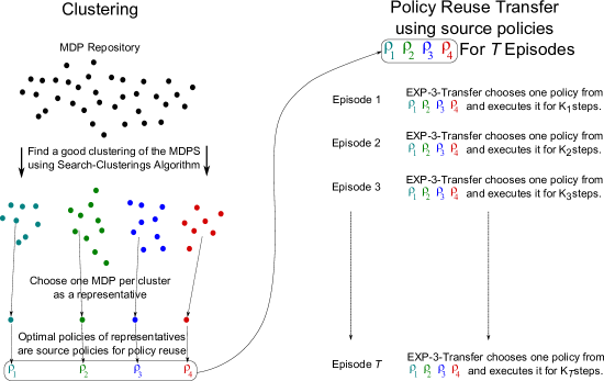
In particular, we define a transfer learning algorithm, EXP-3-Transfer, with performance bound that depends on the number of source policies. Hence this explicitly measures how good the size of the clustering is. We are now left with the task of choosing the clustering and the corresponding source policies. To that end, we define a distance function between two MDPs that takes the distance between two MDPs to be how well the optimal policy of one MDP performs in the other (this in turn is measured as the difference between the value of the optimal policy of the former and the value of the optimal policy of the latter at the start states of the latter). Hence, given that our goal is to reuse optimal policies of one MDP in another, we choose our clustering so that within each cluster the pairwise distances between the elements of the cluster are low. Similarly, we choose the source policy for each cluster to be the optimal policy of the MDP in that cluster which has low distance with respect to all the other elements. Hence, the cost of a clustering with clusters is, roughly speaking, where is a measure of the inter-element distances in the clusters.
Given the cost function, we show that it is NP-hard to find the optimal clustering. So, we introduce a Markov chain Monte Carlo based discrete optimization algorithm to find it. The algorithm is an extension of the Metropolis-Hastings algorithm, which we call Metropolis-Hastings with Auxiliary Variables (MHAV in short), and can also be thought of as an extension to simulated annealing (Kirkpatrick et al., 1983) with stochastic temperature changes. Simulated annealing is a well known algorithm for discrete optimization, but requires carefully setting up an infinite sequence of parameters known as the temperature schedule. Determining this schedule in practice to ensure convergence is acknowledged to be very difficult, and practically an art form. In our version of the algorithm, we search over both the temperature and the optimal point simultaneously, thereby handling the problem of setting the schedule automatically.
To summarize, our overall continual transfer algorithm is as follows. The agent continually learns optimal policies for MDPs presented in sequence. When learning the optimal policy for a particular MDP, the learning agent uses the optimal policies of the previously solved MDPs in a policy reuse transfer learning algorithm. To make transfer more effective, at fixed intervals, the agent clusters the previous MDPs to derive a small subset as the set of source MDPs, whose optimal policies are then used as input to the policy reuse algorithm. The clustering is chosen so as to optimize the regret of the transfer algorithm, and is found by using a convergent discrete optimization algorithm.
We conclude this brief introduction to our method by noting that our transfer algorithm EXP-3-Transfer is in fact an extension of the well known EXP-3 algorithm (Auer et al., 2002b) for non-stochastic multi-armed bandits, and our performance bound is in fact a regret bound of the type well known in bandit algorithm literature. Our strategy is to cast the policy reuse transfer learning problem as a bandit problem, with ‘pure reinforcement learning algorithm’ as one arm, and the source policies as the remaining arms. The regret bound for EXP-3 ensures that we minimize negative transfer by never performing much worse than pure reinforcement learning. We will now discuss related work.
1.1 Related Work
As evidenced by the survey paper (Taylor and Stone, 2009), a significant amount of work has been done on transfer learning in reinforcement learning. As mentioned previously, lifelong learning in reinforcement learning was first explicitly considered in (Mitchell and Thrun, 1993; Thrun and Mitchell, 1995; Thrun, 1996) in the context of learning in robots. In these works, the main aim was to learn the dynamics of robot motion in one circumstance using a function approximator (such as neural networks) and then use these learnt dynamics as an initial bias in a new situation using an explanation based learning framework.
In terms of recent work on TLRL, two different strands are related to our work. The first is work on policy reuse and the second on task encoding. The first and, to the best of our knowledge, the only authors to have considered policy reuse are (Fernandez et al., 2006, 2010). The algorithms presented there, at the beginning of every episode, choose between different source policies by using a softmax criteria on accumulated reward and then use the chosen policy as an initial exploration policy before switching to Q-learning exclusively. In contrast, we extend the EXP-3 algorithm for multi-armed bandits to choose between source policies and Q-learning, and as a result inherit its theoretical guarantees. Additionally, they do not consider the problem of source task selection, whereas in our work this is a major focus.
Two closely related works are (Talvitie and Singh, 2007) and (Azar et al., 2013) where the authors consider the best way to choose between a set of stationary policies. The main distinction between policy reuse and these is the requirement in the former to not perform much worse than a base RL algorithm (which is also our requirement).
We now look at previous work that uses a smaller set of source tasks to represent the complete set of previous tasks. The problem of source task selection through clustering seems to have been considered only by Carroll and Seppi (2005). They introduce several measures for task similarity and then consider clustering tasks according to those measures. The distance functions introduced were heuristic, and the clustering algorithm used was a simple greedy approach. The evaluation of their method was on several toy problems. In contrast, we derive a cost function for clustering in a principled way to optimize the regret of our EXP-3-Transfer policy reuse algorithm. Additionally, instead of constructing the cluster in a greedy fashion, we search through clustering space using a convergent discrete optimization algorithm.
Recent work that also chooses selectively from previous tasks is (Lazaric et al., 2008), (Lazaric and Restilli, 2011). The setting for this paper is a collection of tasks defined on the same state-action space with the tasks and the state-action-state triples for the different tasks generated i.i.d. (similar to the multi-task transfer in classification setting considered in (Baxter, 2000)) rather than sequentially as is typical in RL. Under this setting the authors are able to bound the error when samples from one task are used to learn the new task. This is quite a different setting from us as it is ‘batch’ RL rather than the typical online and sequential RL and measures similarity in terms of the actual transition and reward functions rather than policies or values. Additionally, the analysis and algorithms are derived under the assumption of a fixed set of prior tasks rather than the continual lifelong learning setting we consider.
Source task selection is not the only possible way to represent previous tasks, and the overall goal of finding abstractions for exploiting commonality has received considerable attention in the transfer learning community. Most of the work done in deriving abstractions for the purposes of transfer has been for MDP homomorphisms (Ravindran and Barto, 2003; Ferns et al., 2004; Ravindran, 2013; Konidaris and Barto, 2007; Sorg and Singh, 2009; Castro and Precup, 2010). In these works, similarity between MDPs is defined in terms of bisimulation between states of different MDPs. Bisimulation is a concept borrowed from process algebra. In the context of transfer learning in MDPs, at its most general formulation, a bisimulation is an isomorphism between the state and action spaces that is preserved under the transition distribution – that is for every state-action-state triple , where are the transition distribution of the two MDPs. Unfortunately, in this pure form, bisimulation is absolute (two MDPs are either bisimilar or not) and does not take into account the reward function. And so, in the papers mentioned above, this basic notion was extended in various ways to address both these issues. However, one of the main issues with bisimulation is computational cost, and this remains so in the extensions as well. Another issue with these approaches is that, as observed by Castro and Precup (2010), bisimulation is a worst case metric (two states may have identical optimal actions but still be completely different according to the metric) and as a result requires heuristic modifications.
Technically, the main difference between our approach and bisimulation based methods is that the similarity between different MDPs are ultimately determined by distance between value functions. In our case, however, we are interested in distance in terms of policy. As a result, even though two tasks might be quite different in terms of the value function they might be identical in terms of the optimal policy, and our approach will capture this (as noted earlier, failing to do this was one of the issues with bisimulation based approaches).
Another interesting line of work that uses a different approach to abstracting MDPs is the proto-value function based approach of (Ferrante et al., 2008). Proto-value functions were introduced in (Mahadevan, 2005) as an efficient way to represent the value function for large state spaces as a linear combination of functions, which are called proto-value functions. The main innovation in this approach is that, in representing the value function as a real function over state space, the state-space is treated as a manifold where the distance between points/states is determined by the reachability graph of the MDP. This idea of a spectral-decomposition of the value function naturally lends itself to transfer learning, as, given a new task, we can imagine using the proto-value functions learned in a previous task to initialize the new value function in the new task. It has been noted that proto-value function based transfer has issues in terms of scalability and tractability. The main difference between this and our work is that, as with the homomorphism based approach, our similarity notion is based on policy similarity, while theirs is based on similarity between value functions. Identifying policy similarity is more desirable because tasks similar in terms of value function will be similar in terms of policy, but not necessarily the other way round.
A somewhat different approach to finding MDP abstractions was adopted in (Ammar et al., 2012), where MDPs were related by mapping state action state triples to a lower dimensional space, and consider triples to be equivalent if their representations were found to be close. The authors were able to transfer between tasks such as inverted pendulum, cart pole and mountain car, showing that in these cases their approach was able to discover the fact that the differential equations describing these domains have similar/identical forms.
Finally, our work can also be related to the notion of equivalence between probabilistic models, which has been influential in early work on Bayesian network learning. For instance, Chickering and collaborators wrote a series of papers in which the notion of event equivalence and score equivalence is used to render the problem of searching over network structures somewhat tractable. In (Heckerman and Chickering, 1995), it is shown that the notion of event equivalence, i.e., that two Bayesian networks should be treated as similar if they agree on the independence and dependence relationships between random variables, can be used to define local structure edit operations that enable learning of network structures. Subsequently, in (Chickering and Boutilier, 2002), (Chickering, 2003) this idea is developed further to show that by considering this notion of equivalence it is possible to achieve optimal structure identification with an essentially greedy procedure. We take inspiration from such work, but also note that our task of comparing two sequential decision making problems differs from that of making predictions with a probabilistic model, calling for new notions of process similarity and corresponding algorithms for transfer.
1.2 Paper Organization
In the following we proceed as follows. We present the notation and some fundamental notions in Section 2. Then we define our transfer learning algorithm and framework for measuring distance in Section 4 respectively. Sections 5 and 6 presents our clustering algorithm and the full continual transfer algorithm. We then present our experiments in Section 7 and then end with a conclusion in Section 8.
2 Preliminaries
We use for definitions, to denote probability and for expectation. A finite MDP is defined by the tuple where is a finite set of states, is a finite set of actions and is the set of rewards. is a the state transition distribution for and while , the reward function, is a random variable taking values in . Finally, is the discount rate.
A (stationary) policy for is a map . For a policy , the Q function is given by . The value function for is defined as . An optimal policy satisfies for all policy and state – it can be shown that every finite MDP has an optimal policy. is written , and the corresponding function is given by . When the agent acts in the MDP, at each step it takes an action at a state , and moves to the next state and the reward . The goal of the agent is to learn from these observations and then choose the action at each state. If there are multiple optimal policies, we will designate the first policy in a lexicographical order as the canonical policy. We will assume that is a known upper bound on the reward function. Without loss of generality, in the sequel we assume that there is a single initial state . We call a policy -optimal if
The transfer learning setting. In the transfer learning setting, we are given previous MDPs , and we transfer from these tasks to learn the MDP . The learning of runs for episodes. We denote the optimal policy of the previous MDP by , and the value of a policy in MDP as . Similarly, we denote the reward and transition functions of the MDP by and respectively. We will assume that the rewards of all MDPs fall within the range and we define .
3 The Policy Reuse Problem
In this section we first concretely define the problem of policy-reuse for transfer learning and then define our algorithm for solving this problem. We define the goal of policy reuse to be to design an algorithm that runs for episodes on the target task and, given a collection of source policies and the Q-learning algorithm/policy, performs nearly as well as the best policy (in hindsight) in this collection over the episodes. This requirement has two important implications. First, since the set of policies contain Q-learning, and as Q-learning converges to the optimal policy, it means the algorithm is required to perform nearly as well as a policy that converges to the optimal policy – in other words, the algorithm should avoid negative transfer. Second, if there is a source policy that is near-optimal, then the algorithm is also required to perform nearly as well as that near-optimal policy – in other words, the algorithm should transfer from the new to the old task if possible.
To derive our algorithm we show that policy reuse may be cast as an instance of the non-stochastic multi-armed bandits problem, and hence the classic EXP-3 algorithm (Auer et al., 2002b) may be extended to solve policy reuse. We call our extension EXP-3-Transfer and we derive regret bounds for this algorithm (which is similar to the bounds for EXP-3). In particular we show that EXP-3-Transfer performs nearly as well as the best policy in the collection described above, in expectation with respect to the randomness in the algorithm and the reward and transition function of . Hence, this algorithm satisfies the requirements we laid out for a policy reuse algorithm. We now expand these ideas.
3.1 Defining The Policy Reuse Problem
In the policy reuse transfer problem, we have the target task and a set of source policies (in general, s are arbitrary – but in this paper, each is the optimal policy of some our repository, and Section 4 shows how to choose the s in a principled way). It seems that policy reuse as a method for transfer was first introduced in (Fernandez et al., 2006, 2010). The algorithm introduced was called Probabilistic Policy Reuse (PPR), and the goal of the algorithm was to balance using the source policies and pure reinforcement learning policy (-greedy Q-learning) so that the learning algorithm converges faster than running pure RL by itself. The basic idea in PPR is as follows. At the beginning of each episode, PPR chooses a policy from among the source policies and the -greedy Q-learning policy using a softmax criterion on the observed returns of the policies in previous episodes. It then initiates a policy-reuse episode, where at each step it probabilistically chooses between -greedy Q-learning and the chosen policy, with probability of choosing -greedy Q-learning going to during the episode. In essence, the source policies serve as an initial exploration policy, so that if they to take the agent through paths of the optimal policy, it would result in faster learning of the optimal policy.
There are several aspects of the above algorithm that are noteworthy. First, even if the source policies contain the optimal policy, the algorithm would deterministically switch to Q-learning after the initial phase. Another aspect is that, while there is an intuitive connection between the soft-max criterion and the benefit of using a policy, the actual connection is not made rigorous. Both these issues arise from the fact that the goal of policy reuse was not defined concretely in (Fernandez et al., 2006). So, taking cue from the definition of online learning algorithms (Vovk, 1990; Littlestone and Warmuth, 1994; Cesa-Bianchi and Lugosi, 2006), we define the policy reuse problem concretely as designing an algorithm that chooses policies at every episode in such a way that it does not perform much worse than any of the policies or Q-learning over the episodes. As discussed above, this requirement implies both that (i) the algorithm avoids negative transfer and (ii) transfers from/reuses a good policy (if one exists). Formally,
Definition 1 (The policy reuse problem)
Let transfer learning for the target task be run for episodes, and let be the discounted return accumulated by running (with being the non-stationary Q-learning policy) at episode , with the reward at step and the length of the episode. Let the total discounted reward for policy be . Let be the total discounted reward accumulated by a policy-reuse algorithm . Then we require that for each
where is the expectation is with respect the dynamics of and is the expectation with respect to randomization in the algorithm.
In the following subsections we present the EXP-3-Transfer algorithm for solving this problem and then analyze its performance.
3.2 EXP-3-Transfer For Policy Reuse
In this section, we introduce the non-stochastic multi-armed bandits problem (Auer et al., 2002b) and show that the policy reuse problem may be cast as in instance of this problem. We then present EXP-3-Transfer to solve this problem, which is an extension/modification of the classic EXP-3 algorithm (Auer et al., 2002b) for non-stochastic multi-armed bandits. We discuss the difference between EXP-3 and EXP-3-Transfer in Section 3.3.
Non-Stochastic Multi-armed Bandits
The non-stochastic multi-armed bandits problem is defined as follows.
-
•
There are arms where each arm has a payoff process associated with it. No assumptions are made on the payoff process and they may in fact be adversarial (this is the reason the problem is called non-stochastic).
-
•
A learner operates for steps and at each step it pulls/selects one of the arms .
-
•
At step , the learner obtains payoff and only observes the payoff of the arm it has selected.
The goal of the learner is to minimize its regret with respect to the best arm, that is choose arms to minimize the quantity
A randomized algorithm, called EXP-3, was developed in (Auer et al., 2002b) which minimizes the expected regret, where the expectation is taken with respect to the randomization in the algorithm. It turns out that the regret of EXP-3 satisfies the requirements for the regret in Definition 1 (we expand on this in the next subsection). This implies that the non-stochastic bandits approach, extended to our setting, solves the problem of policy reuse.
Policy Reuse as Non-Stocastic Multi-armed Bandits
We may cast the policy reuse problem as a non-stochastic bandit problem as follows.
-
•
Each source policy and the the Q-learning policy corresponds to an arm, giving a total of arms.
-
•
At each step in the bandit problem, we (the learner) select a policy/arm , and execute it for an episode in the target (so a step in the multi-armed bandit problem corresponds to an episode in the policy reuse problem).
-
•
The payoff we receive for executing policy (i.e. choosing arm ) is the (normalized) total discounted reward by executing for that episode: , with the reward at step and the length of the episode (the normalization is required as EXP-3 expects arm payoffs to lie in ).
EXP-3-Transfer
Given the above transformation, our algorithm EXP-3-Transfer for choosing the policy at step is given in pseudocode form in Algorithm 1. The basic idea is straightforward – at each step it chooses a policy with probability proportional to an adjusted cumulative observed reward of the policy and a term to encourage exploring the policy if it has not been selected recently. The rewards are adjusted to compensate for the fact that, at each step , the algorithm observes the payoff of only , the policy chosen at that step (see Section 3.3 for details on the adjustment). In addition, if the algorithm determines that with high probability a particular source policy (i.e. all but the Q-learning policy) is worse than some other source policy, then it eliminates it from further consideration. The idea is that if we remove an arm we know to be sub-optimal, then we save the episodes that would have been wasted trying that policy.
In detail, the main loop of EXP-3-Transfer runs from line 3 to line 18. contains all the policies not yet eliminated by EXP-3-Transfer. Line 4 computes the probability of choosing a policy, which is proportional to the adjusted observed payoff of each policy, plus the exploration term (). In the next two steps, a policy is chosen probabilistically, executed and its payoff observed and normalized (normalized because EXP-3 expects payoffs to lie in ). In line 7 we record the payoff of the executed policy for use in the elimination step. In lines 8 and 9, the adjusted payoffs of the policies are computed, and their weights updated, respectively. Finally, steps 11 to 17 looks at each stationary policy in , and checks to see if average non-adjusted payoff so far satisfies the elimination condition. If so, the policy is removed from . The elimination condition is justified/obtained from the theorems below which derive the regret bound of the algorithm.
-
•
Set Q-learning policy as the policy.
-
•
Set , let be the payoff of the policy at step ; let .
-
•
Set , where , and is the number of times has been used; set , where , and is the total normalized discounted reward observed for when it was executed.
| (1) |
3.3 Analysis of EXP-3-Transfer
To begin analysis of EXP-3-Transfer, we first note that the payoffs/discounted cumulative reward of a source policy is i.i.d., while the payoff of the Q-learning arm has an unknown non-stationary distribution (because the choice of actions in Q-learning is non-stationary). Our strategy for analyzing the performance despite the non-stationarity, is to assume that there is an unknown adversary that is generating the payoffs for Q-learning and then bound the expected worst-case regret of EXP-3-Transfer with respect to this adversary (this is exactly the strategy used to analyze EXP-3). In particular, in our adversarial/worst-case analysis we assume that there are three participants Nature, Adversary and Player, who make the following choices, in that order.
-
1.
Player chooses the number of episodes and the source policies , and all the other parameters for EXP-3-Transfer
-
2.
Adversary chooses the payoffs for episodes of Q-learning
-
3.
Nature chooses the episodic payoffs for each of the policies for , according the i.i.d. distribution that governs the payoffs (the distribution is determined by , the transition and reward functions respectively of , and ).
-
4.
Player now runs EXP-3-Transfer for episodes, and observed payoffs are the ones chosen by Nature and Adversary as above.
The important thing to note is that in the above framework, there are two sources of randomness/stochasticity – first in step 3 due to the randomization due to the transition and reward functions of and second in step 4 due to choices made by EXP-3-Transfer. As such, our regret bound holds in expectation with respect to these two sources, which we denote by and , respectively. The former is expectation with respect to the transition and reward function in , while the latter is expectation with respect to EXP-3-Transfer. It is crucial to note that in taking these expectations, we assume that the choices made by the adversary in step 2 are taken to be fixed (this is identical to what was done in the analysis of EXP-3 in Auer et al. (2002a)). Our main result for this section is as follows:
Theorem 2
For any source policy ,
| (2) | ||||
| (3) |
when the algorithm is run with . Here is expectation with respect to the distributions and of , while is the expectation with respect to randomization of EXP-3-Transfer, conditional on the event that .
Additionally, with probability , with respect to randomization due to the target MDP , for all source policy , there is at least one such that
The proof is given in Appendix A, but in the following we discuss the bound itself. For the sequel, we define the following function:
| (4) |
This is the right side of the bound above (we will also use it in Section 4 to quantify how good a particular set of source policies is for the purpose of transfer).
The first issue we need to check is whether the bound satisfies the requirements we set out in Definition 1. The definition requires that where and are the total discounted reward over episodes and the expectations are with respect the randomization due to reward and transition function of and the randomization in the algorithm (i.e. ).
We consider the edge case when , and so no arms are ever eliminated and all . In this case, for any ,
| (5) |
which is times the first term in the left hand side of the bound. Now, for any
| (6) |
By the first part of Theorem 2,
which is what is required. Now recall from discussion of Definition 1 above that satisfying the regret requirements imply that the algorithm avoids negative transfer and transfers when possible. Hence, the theorem shows that EXP-3-Transfer does indeed avoid negative transfer and transfers when possible.
When we move away from , we trade off adherence to the requirement in Definition 1 for practical performance. Indeed, while conducting the experiments reported in Section 7, we observed that setting to a suitably low but non-zero value greatly improves performance. However theoretical guarantees are not completely lost in this instance, because for the source policies that are eliminated, part 2 of the theorem says that there is at least one source policy which is, with high probability strictly better than the other policy.
We end this section with a brief discussion of the difference between EXP-3 and EXP-3-Transfer. The primary difference is that we eliminate policies/arms to improve practical performance of the algorithm. This is not possible in EXP-3 because, unlike in our case, it is not assumed that some of the arms have i.i.d. payoffs and so their means cannot be estimated from observations. This leads to a slightly different analysis and improved constant for EXP-3-Transfer and for EXP-3. The practical difference we observe was actually considerable, and without it we were not able to outperform PPR in our experiments (see below).
4 The Clustering Approach To Task Encoding
Recall from Section 1 that in our problem, we assume that we have a repository of MDPs and their optimal policies and we wish to use the optimal policies as the source policies for EXP-3-Transfer. Now we have the following dilemma. As the number of source policies increase, we spend more time evaluating them and accruing sub-optimal reward in the process. On the other hand, if we choose a subset of policies from the repository, then we risk leaving out policies that may have been very useful in the new task. So, essentially we are faced with the problem trading off the size and diversity of the set of source policies.
In this section, we concretely define this tradeoff problem as optimizing a cost function, and in Section 5 we describe an algorithm to optimize it. The cost function is defined over the set of clusterings/partitions of the repository, where each clustering is used to choose a particular subset of policies in the repository as the source policy set. We first show how to choose this source set given a clustering, and then define the cost function that measures how well the source set achieves the tradeoff mentioned above. This cost function then helps us choose the optimal clustering and hence the optimal source policies.
4.1 Constructing Source Policies Given Clustering
Given the MDPs in our repository, let be a particular clustering – that is and . The set of clusterings may vary both by elements of each , and the number of cells . Given a particular clustering , we will obtain the source policies by choosing one policy per . To choose this policy, we define a distance function that measures how similar two MDPs are in terms of their optimal policies.
Let and be any two MDPs in our repository (the distance definition generalizes to any two MDPs defined on the same state and action space, but with different transition and reward functions). Recall that and denotes the value of policy when executed, respectively, in and at the initial state (this can be generalized to different initial states and/or distribution over initial states very easily – but we consider the same initial state setting to keep the presentation simple). Letting the optimal policies for the two MDPs be , , we define the optimal policy similarity between two MDPs as follows.
| (7) |
So this distance upper bounds how much we lose if we use the optimal policy of one MDP in the other – in particular we have the following lemma by construction.
Lemma 3
If , then the optimal policy of is at least -optimal in and vice versa.
The definition of is motivated by the fact that the goal of policy reuse is to use the optimal policy of one MDP in another. We now define the source policies given a clustering :
Definition 4
Given a clustering , define for each the MDP as follows:
| (8) |
(ties broken in terms of order in the sequence ). Then the source policies corresponding to are where corresponds to and is the optimal policy of .
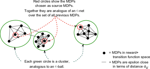
The definition is illustrated in Figure 2 and it means the following. is the element of that minimizes the maximum distance to the other elements of the cluster, and hence, by Lemma 3, is in a worst case sense the best representative of the MDPs in cluster . By choosing the optimal policy of as a source policy , we ensure have the best worst-case representation of the MDPs in each cluster . We make this final statement exact in the next section, in particular in Lemma 5 when we bound the regret of EXP-3-Transfer with respect to optimal policy of any MDP in the repository (rather than just the source policies as done in Section 3).
4.2 Cost Function of a Clustering
Let be a clustering with the source policies chosen as defined in the previous subsection. Our goal in this section will be to quantify the regret of EXP-3-Transfer with respect to any when executed on the new task for episodes, where is the optimal policy of in the repository . We will consider the case where EXP-3-Transfer is run with source policies , and hence this regret will quantify how good the clustering is for transfer – in particular, the lower the regret, the more preferable the clustering. As a result, the regret will serve as the cost function for choosing a clustering to derive the source policies. Before proceeding, note that in Theorem 2, we computed the regret between EXP-3-Transfer and – in this section we extend those results to derive the regret with respect to .
To begin, let the diameter of a cluster , and the mean diameter of the clustering be:
| (9) |
So is the average diameter of the clusters, weighted by the size of the clusters. Therefore, gives the average distance from a cluster center to an element of the cluster. As such, measures how much of the diversity in the repository is captured by the chosen clusters. The smaller , the smaller the average distance between the cluster centers and the MDPs in , and hence more of the diversity of policies in the repository is captured by the .
Using these, we can give an average case quantification11footnotemark: 1of the performance of a clustering when used to generate the source policies and used in EXP-3-Transfer. Let the new MDP have transition and reward functions and . Define and where and are the reward and transition functions for MDP . Additionally let
| (10) |
We have the following result which derives from Theorem 2.
Lemma 5
If EXP-3-Transfer is run with source policies derived from using definition 4 with set as in Theorem 2, then for , such that EXP-3-Transfer did not eliminate by step , the following is true:
| (11) |
Additionally, with probability , with respect to randomization due to the target MDP , for each such that was eliminated, there exist such that
The proof is in Appendix A.
We now use the lemma to derive the cost function. First, in the limiting case of , none of the policies are eliminated and in this case the bound (11) applies to all the MDPs in the repository. In the lemma we assume that each MDP in the repository is equally likely to be the one with the minimum . Hence, taking the average of (11) over all the MDPs, we get the upper bound of the average regret with respect to all the optimal policies of MDPs in the repository:
| (12) |
depends on the repository of s which we do not control or make any assumptions about. Hence, we associate with each cluster the parameters , defined at the beginning of this section, and use (12) to define the following cost:
Definition 6
The cost of a clustering with parameters is defined to be:
| (13) |
4.3 Hardness of finding the Optimal Clustering
In this section we introduce the problem of finding the clustering that minimizes . We argue that optimizing the cost function is hard, which sets the stage for developing our discrete optimization algorithm in the next section. Specifically we will show that it is hard to optimize an upper bound of where was defined in Definition 6. To that end, define the average max-diameter of a clustering to be:
| (14) |
Now define,
Definition 7
Define .
We have the following relationships.
Lemma 8
The parameter of is an upper bound on the parameter of defined in (9). Furthermore, for all clusterings .
Proof
This follows directly from the definition of – in particular,
upper bounds because for each , . The second part of the lemma now follows by the definitions of and .
We reduce the minimum clique-cover problem (Karp, 1972) to the problem of finding the clustering that minimizes and hence establish that it is NP-complete. We start by describing the clique cover problem. Let be a graph where is the set of vertices and is the set of edges. A subset is a clique if for any , there is an edge . The minimum clique cover problem is finding a partition of such that each is a clique and is minimum – that is there exists no other partition with of such that each is a clique and . We have the following theorem for .
Theorem 9
Given a graph , in time polynomial in and , we can reduce the minimum clique cover problem for to finding the clustering of some set of MDPs , , , with all defined on the same state and action spaces, where .
The proof is given in Appendix A. Since the clique cover problem is NP-complete, we immediately have the following corollary.
Corollary 10
Finding the clustering minimizing the upper bound of is NP-complete.
Unfortunately, we do not yet have a proof that minimizing is hard – but the fact that minimizing the upper bound is hard, leads us to conjecture that minimizing is hard as well. For this reason, to optimize the function we need a discrete optimization function, which we will develop in the next section.
We end this section by contrasting our approach to previous approaches to clustering MDPs in TLRL (for instance (Wilson et al., 2007)). In prior work, MDPs are typically characterized by a finite number of real valued parameters, and the distance between parameters determine how similar the MDPs are. These MDPs can then be clustered by, for instance, putting the non-parametric Dirichlet process prior over the parameters of all MDPs, and then using Monte Carlo inference methods to find the clustering that maximizes the posterior probability.
Since our notion of similarity between MDPs is based on policies, to apply this approach to our case, we need (1) a relatively compact parametric representation of optimal policies, and (2) a metric that relates the policy-parameters to values of policies and (3) that optimal policies uniquely characterize MDPs. (1) seems difficult for interesting policies, and (2) seems reasonable only for ‘linear’ domains – i.e. domains where a small change in policy results in a corresponding small change in its value. (3) runs completely counter to one of our main motivations for using policy based clustering, which is that different MDPs might have identical or near-identical optimal policies. So given all these, we were motivated to construct a clustering algorithm adapted to our policy based clustering of MDPS. We also compare our method and the method of Wilson et al. (2007) in Section 7.1, where in a simplified version of their domain, our approach recovers better clusterings.
5 Finding the Optimal Clustering
In Section 4 we defined a cost function that measures how well a particular clustering of the repository of MDPs trades off size and diversity of the set of source policies that are obtained from the clustering. In Section 4.3 we argued that optimizing is hard. This implies that we need a discrete global optimization algorithm for finding the optimal clustering. So in Section 5.1, we introduce the problem of discrete optimization and our approach to solving it. Then in Sections 5.2 to 5.6 we derive and analyze our general optimization algorithm. Finally, in Section 5.7, we apply the algorithm to the problem of finding the optimal clustering.
5.1 Global Optimization With Stochastic Search
Our goal is to solve the discrete global optimization problem of computing , where is the set of all possible clusterings of s. Algorithms for discrete optimization problems tend to fall into specific classes, appropriate for the problem at hand. We present a stochastic search algorithm for our problem (see Figure 3).

Our basic strategy is to construct a distribution over , that concentrates around the optimum and around clusterings with low cost. The concentration property implies that if we repeatedly sample from this distribution, we will find the optimum or a good/low cost clustering with high probability. However, in general, exact sampling from such distributions is difficult, and so our algorithm samples approximately from this distribution using a Markov chain Monte Carlo approach – see (Robert and Casella, 2005) for a comprehensive introduction to MCMC and Metropolis Hastings Markov chains (MH chain in short) that we use. The use of MCMC turns our algorithm into a stochastic search algorithm.
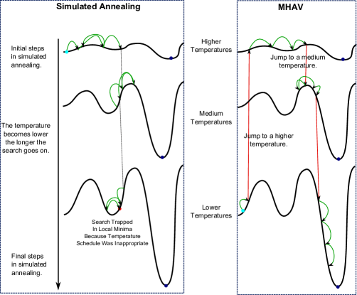
The resulting algorithm can be understood as simulated annealing (Kirkpatrick et al., 1983) but with stochastic temperature changes. Figure 4 describes simulated annealing qualitatively and also contrasts it with our algorithm, MHAV. Simulated annealing is a stochastic search algorithm for optimizing an objective function , where the search rule at step jumps from point to with probability . is a candidate distribution (probability with which is proposed as the next point given current point ) and the remaining term depends on the improvement and the temperature (see below). Because of the in the improvement term, jumps to lower -valued (i.e. better) points succeed with probability 1, while jumps to higher -valued (i.e. worse) points succeed with probability depending on how much higher (worse) the point is.
The temperature is a chief feature of simulated annealing, it is user defined and determines practical success of the algorithm. It is a sequence decreasing in and in essence changes how easy it is to explore the objective function surface – with higher temperature allowing the search to travel over longer distances and in effect making the objective function flatter, and lower temperature restricting the search to points local to the current point, in effect making the objective function steeper (Figure 4 illustrates three qualitatively different temperatures). The temperature sequence needs to be set very carefully so that during the higher temperature phase the search travels longer distances to the places where the minimum point is, and then during the lower temperature phases, the search moves in a ‘local neighborhood’ of the minimum point and and finds the point itself or a point close to it. Clearly, this is a fairly difficult problem and requires some understanding of the objective function.
Figure 4 illustrates our algorithm, MHAV. The algorithm is similar to simulated annealing in that the search rule is such that jumps to better points succeed with probability 1, while jumps to worse points succeed with probability depending on how much worse the point is. It also uses temperatures to modify the flatness of the function (in the algorithm description in Section 5.2 the temperature parameter is represented by , with high temperature corresponding to low ). However, unlike simulated annealing, MHAV does not use a fixed temperature schedule but moves between different temperatures stochastically (Figure 4 illustrates the algorithm jumping between three qualitatively different temperatures). In essence MHAV searches through the augmented space and the search rule has the form . That is, MHAV searches over both the temperature and the solution space simultaneously and so avoids the very difficult problem of needing to set the temperature schedule. Convergence is still guaranteed by convergence of the Metropolis-Hastings algorithm (see Section 5.3). Our proof of the convergence, and the speed of convergence of the algorithm is simple compared to simulated annealing (see, for instance, (Locatelli, 2000) for contrast).
We present our algorithm in steps. We first cast the discrete optimization problem as the problem of sampling from a specific distribution derived from the objective function (Section 5.2), then we present the general Metropolis-Hastings scheme for approximate sampling from a distribution (Section 5.3), and after that we present and analyze our adaptation of Metropolis-Hastings for discrete optimization (Sections 5.4, 5.5 and 5.6), which we call MHAV (Metropolis-Hastings with a auxiliary variable). The MHAV algorithm is a general optimization algorithm, which we then adapt to the problem of searching for the optimal clustering (Section 5.7).
5.2 Optimization as Sampling
In this section, we show how to convert the problem of global optimization to the problem of sampling from a distribution. The method we discuss was inspired by the basic idea behind simulated annealing (Kirkpatrick et al., 1983). Assume that our goal is to minimize a cost function defined over some finite set . In particular assume that there is a subset for which has acceptable cost . Let , such that which satisfies
| (15) |
We now define the distribution
| (16) |
where is the normalization term. Given the existence of , if we draw repeatedly from , then after draws, with probability at least
| (17) |
we will draw an element where . Since , the probability that we draw an element from goes to at rate (hence, the closer is to , the faster the convergence rate will be). So this solves the solves the discrete global optimization problem of optimizing the function .
The reason we introduce the parameter rather than just sampling from is because this distribution is typically intractable to sample from. Indeed, for our MDP clustering problem, the function is and the set is the set of clusterings . By the the hardness result for in Appendix A, we conjecture that sampling from is in fact intractable. Hence, we need to use approximate sampling methods.
Use of approximate sampling turns sampling from into a stochastic search over the objective function to find the global minima. As detailed in the previous subsection, one powerful way to augment such search methods is to modify the objective function by introducing temperatures to change the flatness of the function, and the parameter serves precisely this purpose. In particular, when is high (corresponding to ‘low temperature’), the modified objective function is ‘steep’, and when is low (corresponding to ’high temperature’) is ‘flat’.
5.3 Sampling Using Metropolis-Hastings Chains
In this subsection we describe a standard method to approximately sample from a distribution over a large finite space . In the next section we will use this method to sample from and complete our global optimization method. We use upper-case Roman letters for random variables and lower-case letters to refer to their realized values. In the following, we use the theory of Markov chains as found in (for instance) (Levin et al., 2009). A Markov chain over a (finite) state-space is stochastic process taking values in such that . The distribution is called the transition kernel for the chain, and can be represented by a matrix, also denoted by , such that the entry is (here we have identified each element of with an integer in in some order). A Markov chain is said to be time-homogeneous if , i.e. is independent of time . We will only consider time-homogeneous chains. A distribution over is said to be stationary for the chain with kernel if it satisfies:
| (18) |
That is if is stationary for , then, if we draw according to , then choose according to , then the distribution over will also be .
Let be the probability that given that , that is
Then the chain (equivalently, the kernel ) is said to be irreducible if for each , with . It is called aperiodic if the set has greatest common divisor – that is there is no period to the set of time steps at which the chain returns to some state , starting from itself.
Theorem 11
The following are true for any aperiodic and irreducible Markov chain with kernel :
-
1.
has a stationary distribution and for any ,
(19) where is the total variation distance between any two distributions over .
-
2.
If is stationary for and then for all .
Proof
For the first part and second part, see (for instance), respectively, Theorem 4.9 and Lemma 4.12 in (Levin et al., 2009)).
This result is important because it can be used to approximately sample from a distribution that is hard to sample from directly. The idea is to construct a Markov chain with stationary distribution . Theorem 11 implies that if we simulate long enough, then eventually we will start sampling from . To that end, the Metropolis-Hastings chain (MH chain in short) gives a standard way to define such a chain given as input (see Robert and Casella (2005) for an in-depth introduction).
A MH chain is defined via an irreducible kernel over and an acceptance probability . is problem dependent while is defined as follows:
| (20) |
Given this, the MH chain has transition
| (21) |
It can be easily checked that satisfies the detailed balance equation which in turn is equivalent to (18) (which can be seen by summing both sides over ). So is a chain which if simulated long enough will sample from the target distribution . We will now derive a version of this chain to sample approximately from
5.4 Optimization using Metropolis Hastings With Auxiliary Variables (MHAV)
In this section, we show how we may use the MH algorithm to sample from the distribution defined in Section 5.2 and hence perform optimization. We call this algorithm MH with auxiliary variables (MHAV) because we introduced the auxiliary variable to enable us to perform global optimization. As we discussed above, MHAV may be thought of as simulated annealing without a temperature schedule.
To adapt MH for our global optimization problem, we set and set our target to be . We briefly note here that if we plug into (20), then the normalization term cancels out, and in our algorithms there will never be any need to compute . Let be any irreducible kernel over (this will depend on the nature of and will be an input to the optimization algorithm – we discuss this below). Define the following transition kernel over , parametrized by :
Since , it is easy to see that for any , there is a sequence with positive probability under . That is,
Lemma 12
is irreducible.
Given the above, the proposal distribution for is defined using the parameters , , as follows.
| (22) |
The transition kernel is now defined as in (21) using as the proposal distribution and (16) as the target distribution:
| (23) |
Given the above, the overall discrete global optimization algorithm MHAV (Metropolis-Hastings with Auxiliary Variable) is listed in Algorithm 2. Note that lines 5-6 are sampling from the transition kernel .
5.5 Analysis of the MHAV Algorithm
The reader may prefer to skip this and the next section and move directly to Section 5.7, which details how the MHAV algorithm is adapted to search for the optimal cluster. We begin analysis of our algorithm by showing that the kernel for the defined above is indeed irreducible and aperiodic.
Lemma 13
If and satisfy , the kernel is irreducible and aperiodic.
The proof is given in Appendix A – additionally note that by finiteness of and s, and irreducibility of , such a always exists. The following theorem establishes the probability with which we draw an element from the acceptable set when using to sample.
Theorem 14
has as its stationary distribution, and hence for any initial state of the chain ,
| (24) |
In particular if at step , then for all .
The proof is given in Appendix A. Combining the above with (17) (and the discussion following the equation) shows that the probability that MHAV samples from the acceptable set goes to at rate from step onwards, where is the step such that implies .
We can also derive a convergence rate which establishes that for every such a exists and the rate of convergence of MHAV goes arbitrarily close to . Define the diameter of given the Markov chain to be
| (25) |
Now define the ratio
| (26) |
is finite and non-zero by the irreducibility of and finiteness of . We have the following:
Theorem 15
The convergence rate of to satisfies:
for any initial state .
5.6 Setting the Optimization Parameters
We now discuss heuristics to set the parameters in and in so as to optimize the convergence rate derived above, by minimizing (defined in (26)). In setting these parameters, we are given the proposal distribution , which was required to be an irreducible kernel on , and the target distribution over . We start with the following result which simplifies deriving our result
Lemma 16
(defined in (25)) is independent of , .
The proof is given in Appendix A.
Corollary 17
Given , the set of paths of positive probability under is invariant with respect to .
Proof
Follows directly from the proof of Lemma 16.
So, we need to set to maximize . However, also depends on and , both of which are unknown and so it is difficult to specify optimal values for these a-priori. However, we can give heuristic arguments for setting these parameters in terms of increasing the ‘flow’ of the search process through the search space . First, is used to choose whether we should increase or decrease the value. We set to to ensure a neutral value and that we do not favor either direction and ensure maximum flow through the search space.
Now note that at each step the chain moves either in space or space. and determine, respectively, how often we move in the and how often in . To make the search more effective (based on analysis of simulated annealing type algorithms), it seems we need to make sure that initially we need to explore the quite a bit and only settle down after we have explored sufficiently, by increasing the value. Hence, our recommendation is to set the to be significantly smaller than , ideally the ratio should reflect how difficult we expect it to be to get close to the best (with smaller ratio for greater difficulty). Even though our parameter settings are heuristic, we again stress that this only affects the convergence speed, but not the ultimate convergence. This is in contrast to simulated annealing where convergence itself is guaranteed only if we set the parameters carefully.
5.7 Searching for the Optimal Cluster
Searching for the optimal cluster can now be be solved using the MHAV algorithm. The algorithm for searching through the space of clusterings is given in Algorithm 3. In this case, , and the objective function is . To complete the specification of MHAV for our problem, we define the distribution to be the probability with which a randomized procedure converts to . The randomized procedure is as follows.
Given , choose uniformly at random, and uniformly at random from , where is place-holder/empty set representing a new cluster. Now choose points from , uniformly at random (without replacement), and put them in . The clustering resulting from this transfer is .
Note that if , then has one more cluster than . Additionally, if , and , then has one less cluster than . Otherwise, they both have the same number of clusters, but differing at and . The number is chosen using the exponential distribution over :
This ensures that is small with higher probability and so we are less likely that and are very different due to moving large number of points from to . The parameter is user dependent and in our experiments we set it to .
The following Lemma shows that is irreducible and hence satisfies the condition in Lemma 13 and hence ensures the convergence results in Section 5.5.
Lemma 18
defined above is irreducible.
The proof is in Appendix A.
6 The Continual Transfer Algorithm
In this brief section we combine all the algorithms presented so far into the full continual transfer algorithm, which is listed as Algorithm 4. The algorithm runs in phases and in each phase it solves a MDP using the EXP-3-Transfer algorithm and the current set of source policies as input. In line 4, the function generates the source policies from clustering such that is the optimal policy for where is chosen from according to (8). If the current phase satisfies , then it runs the Search-Clustering algorithm to find a new set of source tasks from the tasks solved so far.
7 Experiments
We performed three sets of experiments to illustrate various aspects and the efficacy of our algorithm222A worst case quantification is also possible. However, the assumptions underlying the worst case seems too weak, and the cost function correspondingly not sufficiently discriminating – i.e. it identifies MDPs that are intuitively dissimilar as being similar. In particular in our experiments, we found this cost function to not give us the intuitive clusters. We discuss this function further in appendix B.. The baseline algorithm for comparison in the first domain was a multi-task hierarchical Bayesian reinforcement learning algorithm proposed by Wilson et al. (2007), and hence compares our approach to an alternative approach to clustering tasks. In the latter two domains we compare against Probabilistic Policy Reuse (PPR) as introduced by Fernandez et al. (2006) which, as mentioned in Section 1.1, is the main prior work on policy reuse algorithms.
In the larger second and third experiments, we report results for our proposed EXP-3-Transfer algorithm, PPR, and standard Q-learning. Additionally, we experiment using different forms of clustering, including no clustering, our Search-Clustering algorithm, clusters chosen manually by hand, and a greedy clustering procedure. The greedy clustering algorithm is to choose a threshold for the distance, then construct clusters by selecting an MDP arbitrarily to seed a cluster, and finally adding all the MDPs with distance less than that threshold to that cluster. In our graphs, we present the results for the best/lowest cost clustering found by using various threshold values.
A summary of the algorithm combinations used are shown in Table 1.
| Algorithm | Full | Sans | Hand-picked | Greedy |
|---|---|---|---|---|
| Exp-3-Transfer | ||||
| Probabilistic Policy Reuse | ||||
| Q-learning | N/A | N/A | N/A | N/A |
For each graph presented in experiments 2 and 3, the results are averaged over 10 different target tasks with 10 trials per task. The various parameters used for the clustering and transfer algorithms are given in Table 2.
| Exp-3-Transfer | Search-Clusterings | RL | |||||
|---|---|---|---|---|---|---|---|
| and | (for each of random restarts) | ||||||
We present results from experiments run on three different domains. In Section 7.1 we use the coloured grid world domain, commonly used in Bayesian reinforcement learning, to compare the clusters found by our proposed algorithm with those of a hierarchical Bayesian method, in order to motivate our clustering approach. In Section 7.2 we present results from a simple windy corridor domain to demonstrate the clusters produced by our Search-Clustering algorithm. The results show that the clusters found are intuitive in nature. In Section 13, we present results on the more complex surveillance domain (described briefly in the Section 1) which is a variant of the kinds of problems that are considered, for instance, by An et al. (2012). In this experiment we show the performance for the algorithm combinations given in Table 1 under various numbers of previous tasks and task lengths.
7.1 Coloured Grid World Domain
Wilson et al. (2007) introduced a method for modelling the unknown distribution of tasks in a multi-task reinforcement learning problem using a hierarchical infinite mixture model. Their two-layer model is capable of representing a previously unknown number of classes of MDPs, as well as finding the latent distribution of parameters in each class. For any new task, the model acts as a prior over the parameter space, which enables the generation of a faster initial solution, to be subsequently optimised with additional task-specific learning.
This model describes latent structure in the parameter space of the observed tasks. Instead, our proposed clustering algorithm seeks to identify similarities in policies across different tasks.
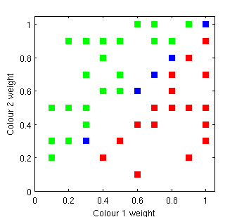
To compare this infinite mixture model approach with ours, we consider a simplified version of the coloured maze domain of Wilson et al. (2007), where each cell of a grid world is coloured with one of two possible colours. Each colour is assigned a weight , the values of which differ between tasks. The agent navigates the grid world from one corner to the diagonally opposite corner. This is done using four actions, each of which moves the agent to an adjacent cell in the corresponding cardinal direction, deterministically. After every movement, the agent receives a reward equal to the sum of the colour weights of the current cell and the adjacent four cells. The goal of the agent is to maximise the received rewards. Each task is completely described by two parameters (the colour weights) in the unit square. This is intended to simplify visualisation of the resulting clusterings.
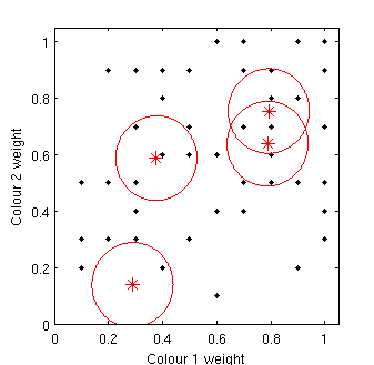
We sample 50 tasks uniformly at random from the unit square and cluster them using both the hierarchical infinite mixture model and our framework. Figure 5a shows the clustering results of Wilson et al. (2007), and Figure 5b shows the clusters obtained by our method. Note that all the tasks that lie on the same line that goes through the origin are equivalent as they have the same colour weight ratio, and thus have the same optimal policy with scaled values. As a result, our method is able to model this fact and summarise the complete set of MDPs into a reduced set of landmark MDPs with equivalent policies. On the other hand, modelling the similarities between tasks based on task parameters will fail to realise this equivalence, and subsequently result in many clusters with similar policies because they share a local neighbourhood in parameter space.
7.2 Windy Corridor Domain
The windy corridor domain is illustrated in Figure 6. The domain consists of a row of parallel corridors with a ‘wind’ blowing from the South to the North along two columns of cells near the entrance to the corridors.

The agent has one action for each possible cardinal direction which moves it in that direction deterministically. In a windy cell, the motion of the agent becomes probabilistic with the probability of moving North being , and moving in the desired direction being . depends on the probability of wind in that cell, which is a task parameter ranging from to .
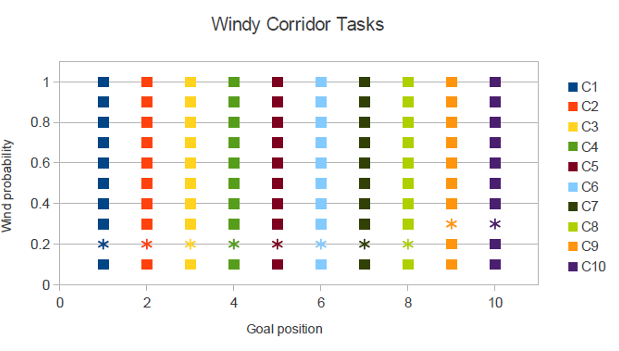
The MDPs in the domain are distinguished by two values: the location of the goal state and the probability of wind. There are possible wind probabilities, which together with the possible goal locations, results in a total of possible MDPs.
For this domain, we learned the optimal value function for each of the MDPs, and from that computed the distance between every pair of MDPs. This was then used to cluster the MDPs using the Search-Clusterings algorithm. Figure 7 presents the final clusters we found for this domain. This figure shows that the best clustering found by the algorithm placed tasks with the same goal state in the same cluster. This follows intuition because, despite the wind probability, the policies required for MDPs with identical goal states will be identical, yet be different for tasks with different goal states. This demonstrates that the Search-Clusterings algorithm is capable of recovering the expected clusters, thereby providing a sanity check for our algorithm, although we note that the results are stochastic and vary between runs.
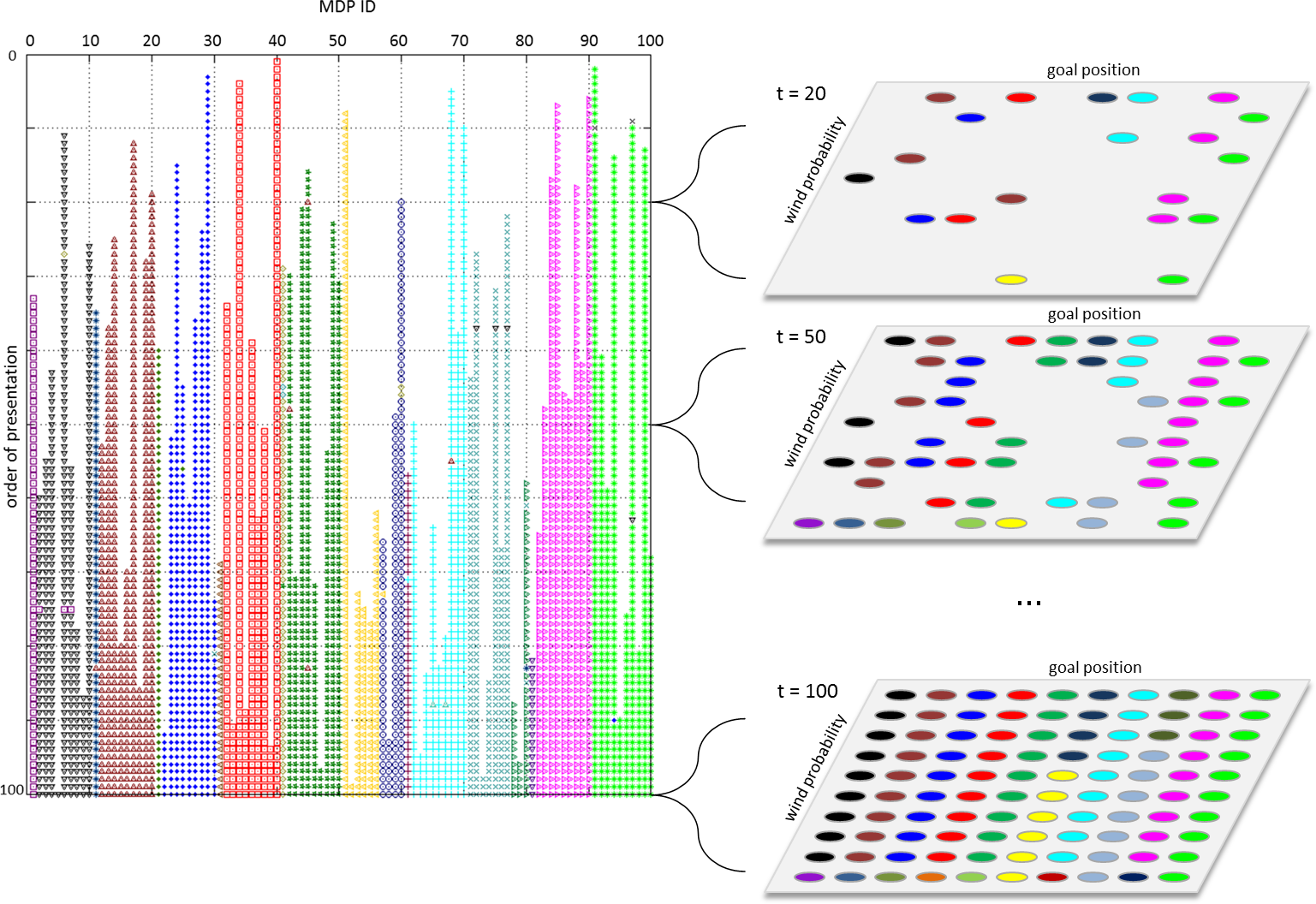
In order to illustrate the effects of the clustering, we incrementally built up the full set of MDPs, by presenting them in a random order to the Search-Clustering algorithm, and having it cluster them after the addition of each new MDP. These results are shown in Figure 8. Note that the allocation of MDPs to clusters remains largely consistent across the presentation of MDPs. In this case, the algorithm recovers main clusters.
7.3 Surveillance Domain
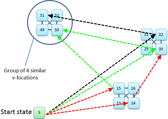
The surveillance domain is illustrated in Figure 9. In this domain, the goal of the agent is to catch infiltrators who wish to break into a target region. There are different vulnerable locations (abbreviated v-locations) in the domain, and the infiltrators only choose a subset of those v-locations to infiltrate – we call these target v-locations. The type of the infiltrators is defined by the sequence in which they visit the target v-locations and the goal of the agent is to find out where the target locations are and surveil them in the right sequence to find the infiltrators.
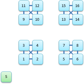
The actions available to the agent are the motion actions in the cardinal directions as well as a surveillance action, each of which is deterministic in its outcome. Every action taken results in a reward of , an unsuccessful surveillance action (i.e. inspecting the target v-location in the wrong order) results in a reward of , while a successful surveillance action (i.e. inspecting the correct v-location at the right time) results in a reward of . If instead of surveilling the correct v-location, the agent surveils a location adjacent to it, then it receives a reward of . Each v-location has 3 other v-locations that are adjacent (see Figure 9). Hence two MDPs , , each corresponding to different v-location sequences and , are similar in terms of their optimal policy/ distance, and belong to the same cluster, if each pair of v-locations and are adjacent – because in this case, the optimal policy of will yield near-optimal sequence of rewards of s when applied in and vice versa.
We present the following results for experiments run with a combination of different numbers of previous MDPs (referring to the surveillance tasks which have been encountered before, and possibly subsequently clustered) and numbers of target locations. The results show that the more complex the transfer task is, the better EXP-3-Transfer with clustering performs compared to Probabilistic Policy Reuse, where complexity is measured in terms of the number of previous MDPs and the difficulty of the target task.
-
•
We compare the performance of EXP-3-Transfer, Probabilistic Policy Reuse and Q-learning as the complexity of the transfer problem increases. Here, the complexity of the transfer problem is both the number of previous tasks, and the complexity of the MDP itself (i.e. the number of target v-locations). These results are referred to as clustering gains.
-
•
We compare the effect of different types of clusterings (in Table 1) for EXP-3-Transfer with . These results are called clustering comparisons.
-
•
We compare the effect of having different for EXP-3-Transfer with clustering for various number of previous tasks. These results are the time comparisons.
7.3.1 Clustering Gains
We first study the effects of clustering, by comparing the performance of both EXP-3-Transfer and Probabilistic Policy Reuse with and without clustering. The results presented in this section summarise those of the complete experiment set, the results of which are provided in Appendix D.
Figure 11 demonstrates the performance of the two algorithms on two different task variants in the surveillance domain: having either a sequence of two or three v-locations. The figure measures the clustering gain, being the difference in performance with and without clustering. This figure does not show a comparison with Q-learning. In the full results given in Appendix D, we show that EXP-3 consistently outperforms Q-learning by a large margin, indicating that our algorithm escapes negative transfer.
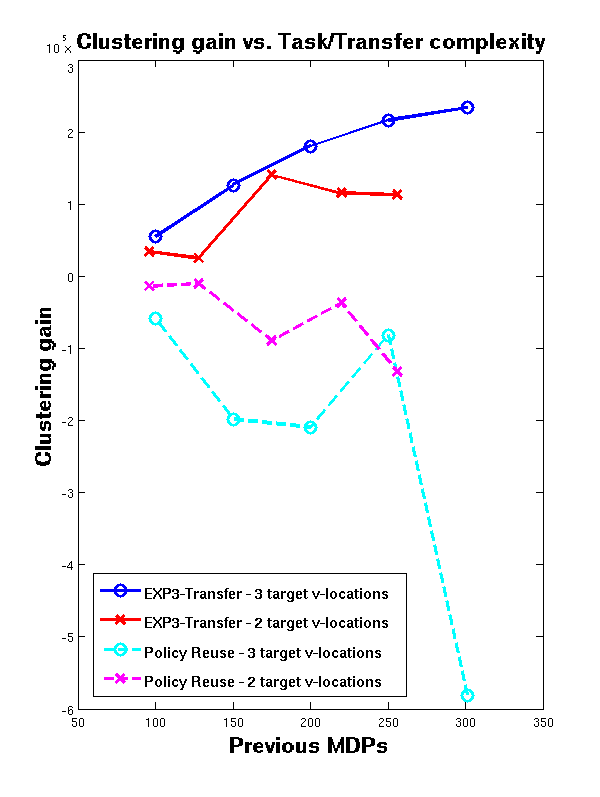
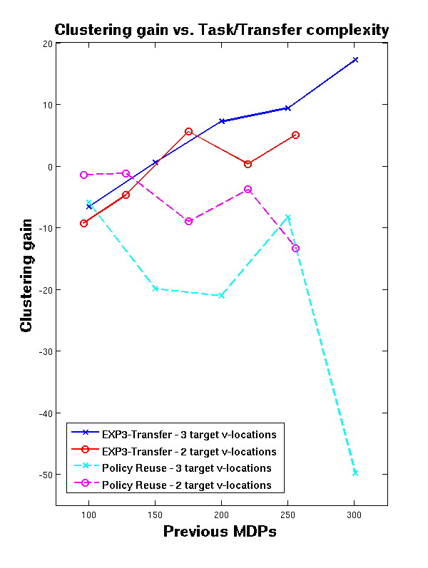
As can be seen, EXP-3-Transfer always benefits from using clustering. Furthermore, the more complex the task, the better the performance. This is observed in the general upwards trend in the curves with an increasing number of previous MDPs, and the fact that the curve for the 3 v-locations lies above the curve for the 2 v-locations. This result is in complete agreement with our expectations, that in a bandit-like algorithm lowering the number of arms will result in lower regret. In addition, this result indicates that our clustering algorithm retains the correct arms so that with the removal of arms, the performance of EXP-3-Transfer is not affected adversely.
Interestingly, for Probabilistic Policy Reuse the trend is reversed. It appears that clustering does not help this algorithm, and the clustering additionally becomes more detrimental as the task complexity increases. Our conjecture regarding the reason for this is that Probabilistic Policy Reuse uses the source policies not as potential optimal policies, but rather as exploration devices. By clustering the MDPs, we remove arms and hence reduce the number of exploration policies, which lowers the scope for exploration. This in turn results in negative performance gain for Probabilistic Policy Reuse.
It is also interesting to note that in Figure 11b, which shows the gain in terms of the final reward obtained, the initial gain for EXP-3-Transfer and PPR are both negative, and the gain for PPR is higher. However, as the transfer complexity increases (both in terms of previous MDPs and task complexity) the cumulative reward gain becomes positive for EXP-3-Transfer, while for PPR it continues to decrease.
Given that the above figures show that PPR does not benefit from clustering, we compare the cumulative reward obtained by EXP-3-Transfer with clustering and PPR without clustering for the complex -target-v-locations problem in Figure 12. This result shows that EXP-3-Transfer completely dominates PPR, with the difference becoming particularly stark when the number of previous tasks increases to .
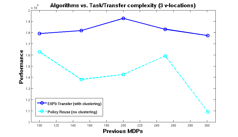
7.3.2 Clustering Comparison
We now compare the performance of EXP-3-Transfer when using the different types of clustering methods reported in Table 1. As in the previous section, we examine the change in performance with increasing complexity of the transfer tasks. The summary of these results is given in Figure 13, and again, the full results are provided in Appendix D.
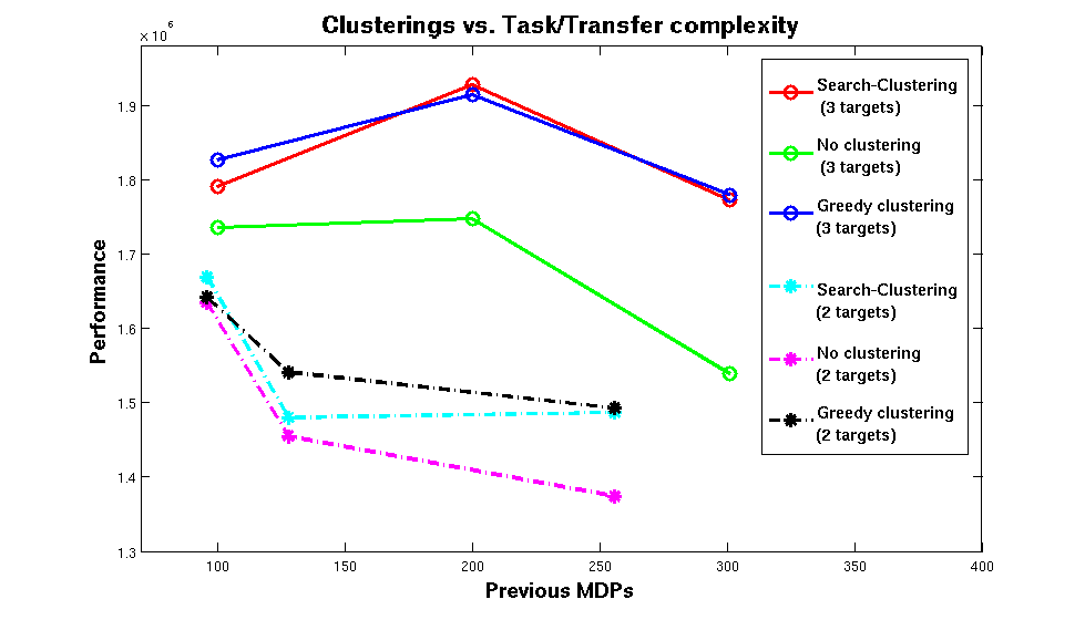
As can be seen, EXP-3-Transfer using Search-Clustering to obtain the source policies outperforms the case when we do not cluster the previous tasks. This confirms the result reported in the previous section. However, in addition we also observe that transfer after using the greedy clustering scheme performs about as well as using Search-Clustering for the 100 and 260 previous MDPs, but for the 125 previous MDPs, Search-Clusterings is significantly better. Search-Clustering and Greedy Clustering are comparable for those two numbers of previous MDPs largely due to the structure of the domain, where every element of each group of tasks is similar to every other task in the same group. That is, when the agent surveils any v-location in the same group as the true v-location required by the task it receives near-optimal rewards (see Figure 10).
However, greedy clustering would fail on a more complex variant of the surveillance domain. To understand this issue, recall from the beginning of Section that two MDPs , , corresponding to v-location sequences and , are similar in terms of their optimal policy, and hence belong to the same cluster, if each pair of v-locations and are adjacent. In this case surveiling instead of yeilds a reward of in and vice versa. Hence within each correct cluster of MDPs we have a symmetry: the distance between each pair of MDPs is very similar. At the same time the distance to MDPs not in the same cluster is quite different. So if in greedy clustering if we start with any MDP in a given cluster, we will find the other MDPs in the cluster. Greedy clustering will no longer work if we break this symmetry by explicitly modifying the domain definition.
One simple way to do this is as follows. In the complex domain, for each correct cluster we have a single MDP (the centroid ) that has low distance to all other elements of the cluster, while every other MDP of the cluster has a high distance to the other non-centroid elements. To get this effect, we have 5 v-locations per group of adjacent locations. We then change the reward function so that in each group of adjacent locations (see figure 14), the reward is asymmetric - we designate a single v-location, say which yields a reward of if it is surveilled instead of and vice-versa, but for all the other v-locations, surveilling instead of , , yields a reward of . Hence the would be the MDP with v-location sequence . In this case, greedy clustering will fail to learn every cluster for which it does not start with the centroid MDP because the for the non-centroid MDPs, the distance to the other MDPs would be too large. The result for the complex domain is given in table 3. We see that, transfer using the clusters produced by Search-Clustering outperforms transfer using clusters discovered by greedy clustering approach by a factor of 2 as we increase the number of previous MDPs. Recall that each point is obtained from averaging over 10 different target tasks.
| No. of Previous MDPs | Search Clustering | Greedy Clustering |
|---|---|---|
| 100 | ||
| 200 |
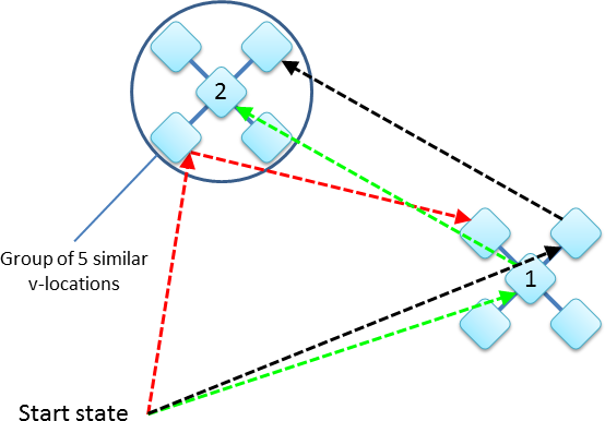
7.3.3 Time Comparisons
Finally we examine the effect of the parameter on performance on the original surveillance domain. Recall that the parameter affects both the clustering algorithm Search-Clustering and EXP-3-Transfer, and is the time duration in terms of the number of episodes over which the transfer procedure is run. We performed experiments with different combinations of numbers of previous MDPs and MDP complexity. The results of these are all qualitatively similar, and so we present only two graphs in Figure 15 for the most complex and the least complex transfer problem we have considered. We relegate the remaining graphs for the rest of the experiments to Appendix D.2.
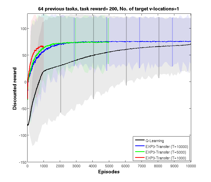
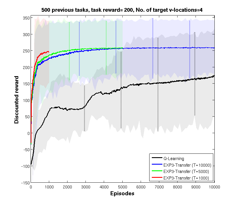
As these results show, the performance curve for EXP-3-Transfer with parameter lies above the curves of EXP-3-Transfer with parameter , for any . This illustrates the effect of optimising transfer performance for a set time duration.
8 Conclusion
In this paper we developed a framework to concisely represent a large number of previous MDPs by a smaller number of source MDPs for transfer learning. We presented a principled online transfer learning algorithm, a principled way to evaluate source sets for use in this algorithm and way to find the source set. The key idea was to cluster the previous MDPs and then use the representative element of each cluster as the source tasks. We also presented extensive experiments to show the efficacy of our method. We now discuss several interesting directions for future work.
In this paper we only considered discrete domains. However, it is possible to translate the overall approach to the continuous setting. In particular, to apply our approach to continuous space problem, all we will need is a pure RL algorithm (as an arm in EXP-3-Transfer) and a way to evaluate policies (to compute the distances). All our definitions, algorithms and results will then hold true in this setting. This is because our algorithms EXP-3-Transfer, MHAV and Search-Clustering and distance function treats the underlying MDPs and policies as black boxes with certain properties. The discreteness of the MDP is never exploited or required in either the algorithms or their analysis.
Finally, we end by pointing out that the idea of clustering a set of tasks to obtain a representative set is much more general. For instance, any other cost function derived under different assumptions can be applied with the clustering approach. As another example, the clustering approach may also be used in multi-agent systems to group together opponents according to whether the same policy of ours is equally effective against opponents in the same group. It will also be interesting to implement these methods and algorithms on scaled up, real version of the types of problems considered in this paper. We plan to pursue these and other extensions to the above in future work.
A Proofs
Proof [Proof of Theorem 2] A direct application of Corollary 3.2 in (Auer et al., 2002b) is not possible because our algorithm diverges from EXP-3 because the number of arms possibly decreases across time steps. The proof of the first part, while structurally similar tp the proof of Theorem 3.1 of Auer et al. (2002b), is different in some crucial detail due to the removal of arms/policies. The second part, where we deal with arms that were removed, is novel.
Recall that is the set of policies not yet eliminated at the beginning of step EXP-3-Transfer, and let . Let , and (note the , rather than in the summation in ). Then for all sequences of policies , drawn by EXP-3-Transfer,
| (27) |
In the above, (1) follows because as , and because all the weights are positive. (2) follows by the update equation for in line 9 of EXP-3-Transfer. (3) follows by definition of . (4) follows by definition of in line 4 of EXP-3-Transfer. (5) holds because and because the term in the exponential is positive. Finally, (6) follows by the identical reasoning used to derive (8) in the proof of Theorem 3.1 (Auer et al., 2002a).
Now, we can proceed along similar lines as in Theorem 3.1. Using the fact that gives us
Now since is non-increasing, , and so
Summing over telescopes and gives us
Now, going in the opposite direction, for each we have
Putting these together, we have for each ,
| (28) |
Rearranging, we get
| (29) |
Taking expectation in terms of the randomization in the algorithm in both sides above, conditional of , we have
| (30) |
For the final term on the right hand side, we used the fact for any . To see this, note that there are two possibilities – either , or . If then , and otherwise, as .
Now, using the fact that (as ) and then rearranging, we get for each ,
| (31) |
Plugging in the value of in the theorem statement we get
| (32) |
Now note that , so taking expectation with respect to , dividing by and multiplying by we get from (32)
This completes the proof of the first part.
To prove the second part, we need the Hoeffding bound (see, for instance, (Dubhashi and Panconesi, 2009) for an exposition) which states that if are i.i.d. draws of a random variable , with , and is the empirical mean of the , then
| (33) |
In the sequel, we will assume that , and so the denominator in the exponent on the left hand side of the equation is just . This bound then has the following simple and well known consequence. Assume we have two i.i.d. samples and , drawn from two random variables and . Assume that , and and both satisfy and . Then, by (33)
| (34) |
Then, by the triangle inequality and the union bound, with probability at least , .
Now in line 13 of EXP-3-Transfer, we remove a source policy arm if , we have and . This implies, that with probability , . Since there are arms, this implies that if there is an arm that was removed, by the union bound with probability at least , for some arm for every arm that is eventually removed.
For the next two proofs, we need to restate Lemma 1 in (Strehl and Littman, 2008).
Lemma 19
[Strehl, Li and Littman] Let the new have transition and reward functions and . Let and where and are the reward and transition functions for MDP . Then, for any policy and state ,
| (35) |
where (first defined in (10)).
Now we can state our proof.
Proof [Proof of Lemma 5] Fix any previous and let be the centroid of the cluster of such that . By definition, the optimal policy of , used as an arm in EXP-3-Transfer, is and . By Lemma 19, and . Putting the three inequalities together, we have . By Theorem 2, if was not eliminated by EXP-3-Transfer, , and therefore .
Now consider the case where the policy was eliminated at some point. Then, by the second part of Theorem 2, there exists a policy for which with probability at least , . From the relationship between and established above, we get that with probability , .
Proof [Proof of Theorem 9] First, let , and given any ordering of the elements of , identify each vertex with its position in the ordering – so we can take . Let be a set of MDPs defined on a state space , and action space . The transition function for the MDPs in this case is trivial (all actions transition with probability from to ). The reward function for MDP defined as follows. ; if then , otherwise where and is the function used in Definition 6 to define the cost function for clusters. In the following we will identify MDP with vertex and this way show that the optimal clustering for this corresponds to a maximal clique under the mapping and .
By construction, , , iff , and otherwise. Hence, by the definition in (7),
| (36) |
Now recall that . Let an optimal clustering be and let denote the cluster in that belongs to. We now show that if , then form a clique in . In other words, we show that, if then , or equivalently then . By way of contradiction, assume that but . Since do not have an edge between them, by (36) the diameter of is at least . Which in turn implies that . Now consider the clustering obtained by putting each MDP in its own cluster. This clustering has cost – contradicting the optimality of . Hence, the clusters of has cost and corresponds to a collection of cliques that partition – denote this collection of cliques by .
Now note that each collection of cliques that partition correspond to a clustering such that iff for some ; in this case . Now assume that there is a collection of cliques such that and let the corresponding clustering be . Then we show that , resulting in a contradiction. To see this note that each then by (36). Hence the diameter of = . So the cost of is since by definition of , .
Because of the contradiction, is indeed a minimum clique cover, showing that the problem of minimum clique cover can be reduced to the problem of finding the optimal clustering. To complete the proof, we need to show that this reduction takes polynomial time. The only cost in computing a is setting the reward function, which takes time for some constant .
Proof [Proof of Lemma 13] To show irreducibility we have to show that for any and there exists a such that . To see this, first note that was assumed to be irreducible. So, there exists a such that with . Now consider a particular path with probability under . From the definition in (21), the probability under of each transition is
where the inequality follows as by assumption in the Lemma statement. Hence, the total probability of the path under is lower bounded by (where ). Summing over all possible paths of length going from to gives that the probability of each from is lower bounded by .
Now assume that while . If , we can bound the probability under of going from to , where , by (this follows from definition of and ). Hence we reach from with probability . By a symmetric argument, if , we reach from with probability at least , where . Both are positive by the finiteness of and s. Putting all the above together, we have that the probability of transitioning from to is lower bounded by
which shows that is irreducible.
To show that is aperiodic, it is sufficient to note that . Then, with probability , returns to the same state in step, which ensures that the g.c.d. of the set of time steps where returns to the same state is .
Proof [Proof of Theorem 14]
is irreducible by Lemma 13 and by construction of an MH chain, has stationary distribution. Hence, by the first part of Theorem 11 converges to in total variation. By the second part of the same theorem, if , then for all , .
Proof [Proof of Theorem 15] As we mentioned above, this proof follows very closely the proof of Theorem 4.9 in (Levin et al., 2009). To begin with, first we note that by irreducibility of , the diameter (defined in (25)) is finite. Hence, by definition of in (26), for each we have that .
Let denote the transition matrix for the kernel so that – i.e. row contains the distribution . Let denote the transition matrix where each row is . Then, setting , we can write
where is another transition matrix. To see that is a valid transition matrix, note that row of is given by . Summing the elements of this row, we get = , whence each row of sums to . Furthermore, by the definition that , each entry is also positive, showing that is indeed a valid transition matrix.
Now note that for any transition matrix , . Additionally, since is stationary for , . We will now use the above facts to show by induction on that
| (37) |
which will imply the convergence we seek.
Clearly (37) is true for . Assume, as the inductive hypothesis, that it is true for . Then, we have
The first equality is just the definition of -step transitions. The second equality is obtained by applying the inductive hypothesis and because . The third and fourth equality follows from applying the inductive hypothesis on and the two facts about established above. The final equality is obtained by cancelling out the terms.
Now as , and so each row of converges to . In other words for each , . This implies . Now since , this completes the proof.
Proof [Proof of Lemma 16]
Fix any two and and let be a path with and . Assume that this path has positive probability under for certain value , respectively of , . Then, by definition (23) of , the probability of this path has the form where the are integers and is a constant. Then, under a difference set of values , the probability of this path has the form . Since , this probability must also be non-zero. Hence the set of paths of positive probability are invariant with respect to the values of and . Since is the length of the shortest path of positive probability, this proves the lemma.
Proof [Proof of Lemma 18]
We just need to show that, for any two clusterings and , only a finite number of re-arrangement steps is sufficient to obtain from . Let the clusters of , in some order, be . Assume that the points of are spread across with points respectively. Then, with non-zero probability will be created with points from (see Appendix C for the explicit computation). And from then on, with non-zero probability (again, see the computations given) the points of in will be added to . Hence with non-zero probability will be created. This holds for each , and hence we have a non-zero probability of constructing from .
B Worst Case Quantification of the Cost Function
This appendix continues from Section 4.2 where we derived the case cost function for a clustering by considering an average case scenario. We now derive a cost function in the worst case setting. To begin, we define the following worst case measure of homogenity of the clustering.
| (38) |
The main result is as follows.
Lemma 20
Proof By the exact same steps as in the proof of Lemma 5, we have . Taking the max over yields
which completes the proof.
We now discuss which of the two quantifications, worst or average case, is more appropriate. If we have reason to strongly believe that the next MDP is chosen by nature adversarially with respect to our choice of cluster – that is, nature chooses to maximize – then clearly, the worst case quantification is the correct way to evaluate a clustering. On the other hand, if we do not have any reason to believe this, then the average case might be more appropriate. For instance a consider a clustering of MDPs that contains all the MDPs in a clusters, such that of the clusters have diameter while the one is sparse but wide (say elements with diameter ). For many domains, we would consider this a good clustering and for this situation, the average case quantification would be , whereas the worst case quantification would be . Intuitively this seems a little too pessimistic and indeed, we also observed similar results for our experiments, in the sense that the worst case quantification failed to uncover clusters that we would intuitively consider good. Hence, for the rest of the paper we use the average case quantification to define our distance function.
C Computations
Here we present the computation of the ratio defined using (22) and constructed using defined in Section 5.7. For this section, we set . We have four cases to consider.
Case 1: With probability , increased and . In this case, we have , and
Case 2: With probability , decreased and . In this case we have , ,
Case 3: With probability , and .
Case 4: With probability , and is rearranged. Now the probability of moving points from to is,
The reverse probability now depends on what actually has been moved. We have 4 subcases:
Case 4.1: If points are moved between clusters and from clustering , with :
Now, we have that and , so that, we have:
Case 4.2: If points are moved from cluster to a new cluster , with :
note that . Now, we have that and . So the desired ratio is:
Case 4.3: If points are moved from cluster to existing cluster , now we have one less cluster so that,
The values are: and . Together, this gives us the ratio:
Case 4.4: If points are moved from cluster to a new cluster :
The clustering does not change in this case and the values are: , , which gives us
| (39) |
D Surveillance Domain Experiments: Algorithm Comparisons
In this section we give detailed cumulative reward curves for the algorithms: E3T with clustering, Policy-Reuse with clustering and Policy-Reuse with clustering. The results are given in Figures 16 to 18. The results more or less show what the summary graphs showed. In particular, when the number of previous tasks and the complexity of task is low, Policy-Reuse is better than our algorithm. However, as the complexity keeps increasing, our algorithm begins to dominate both versions of Policy-Reuse, showing that clustering is beneficial.
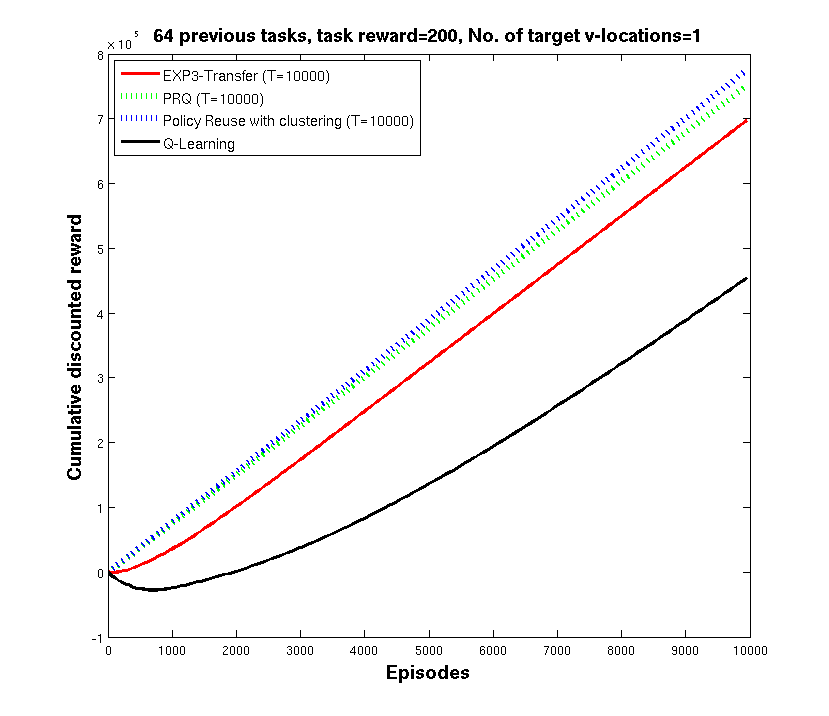
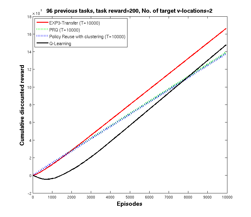
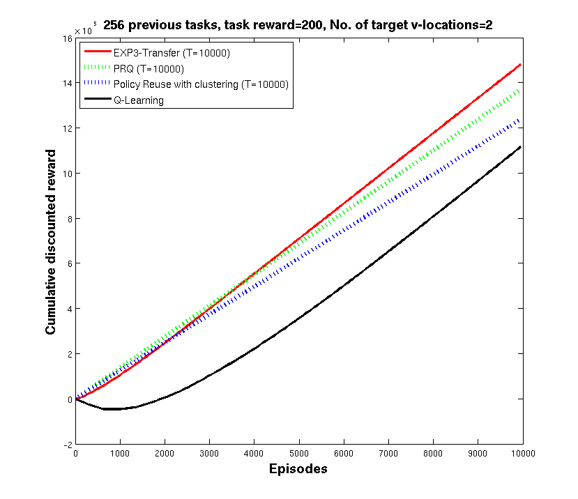
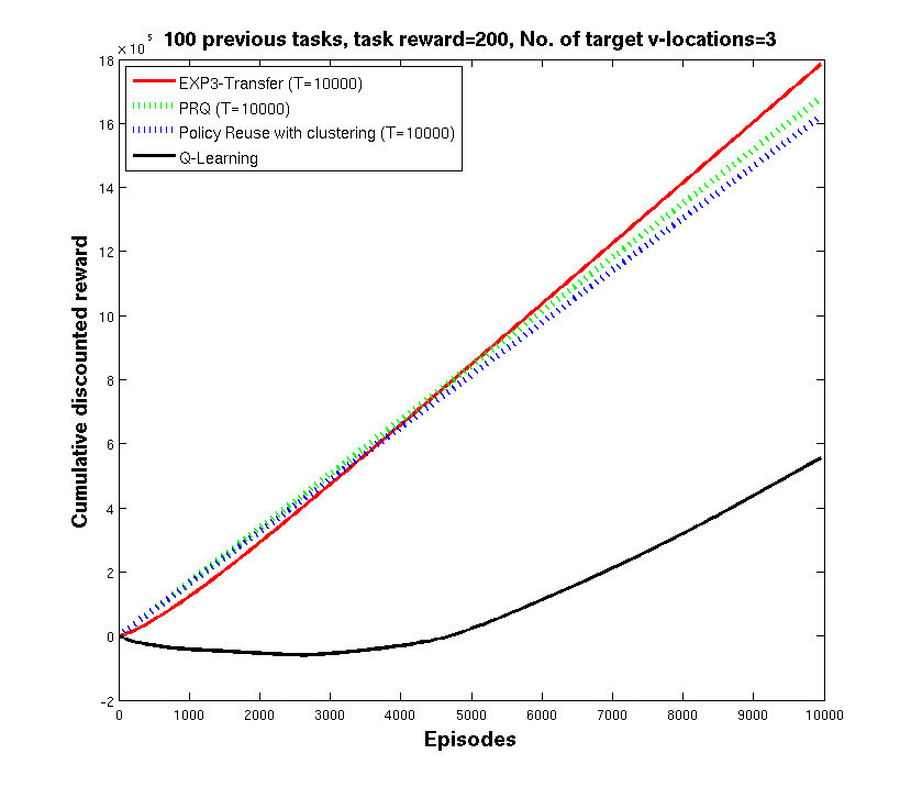
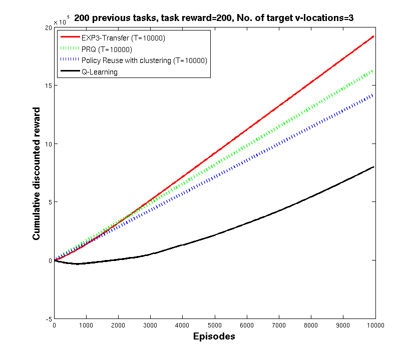
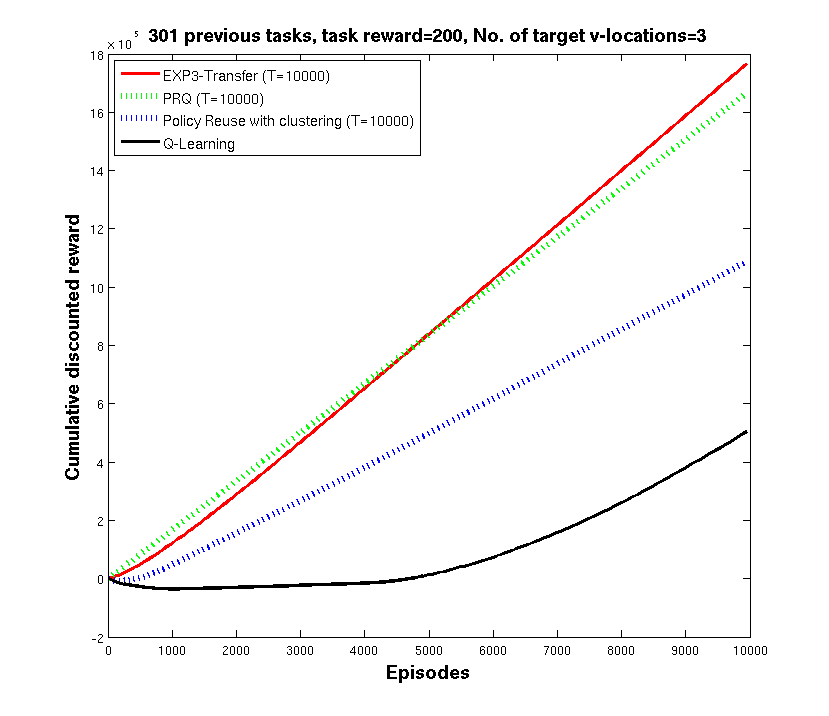
D.1 Surveillance Domain: Clustering Comparisons
In this section in figures 19 to 21 we present the learning curves summarized in figure 13. The general trend follows what was observed in Section 7.3.2.
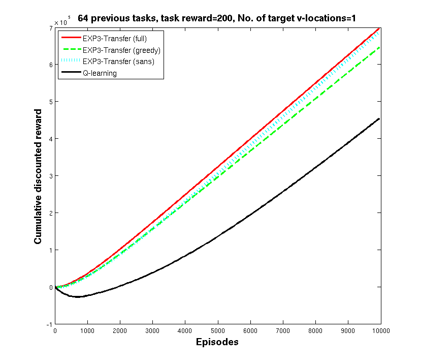
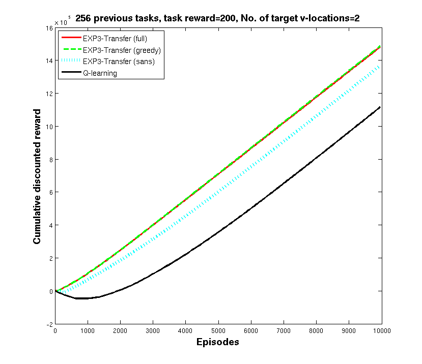
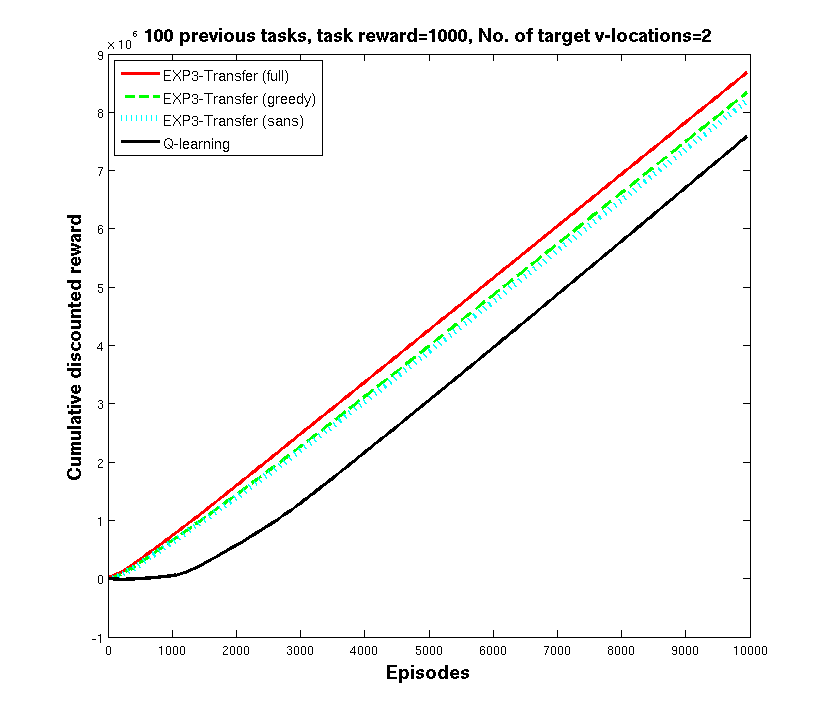
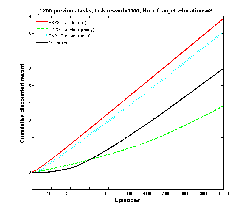
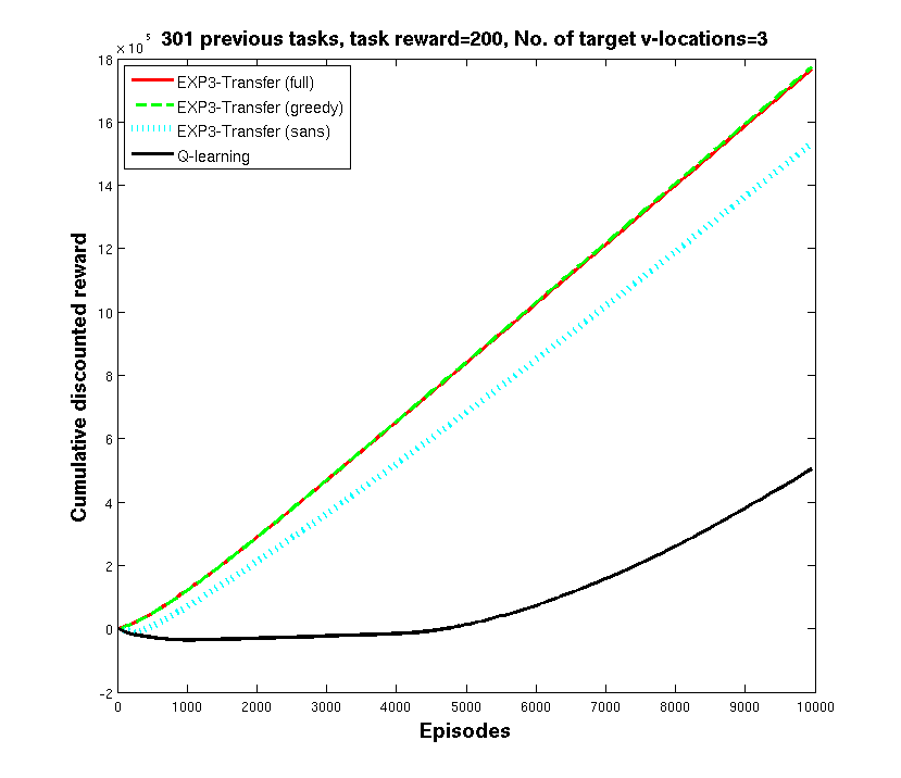
D.2 Time Comparisons
Figures 22 to 24 gives the time comparison results for transfer problems not described in Figure 15.
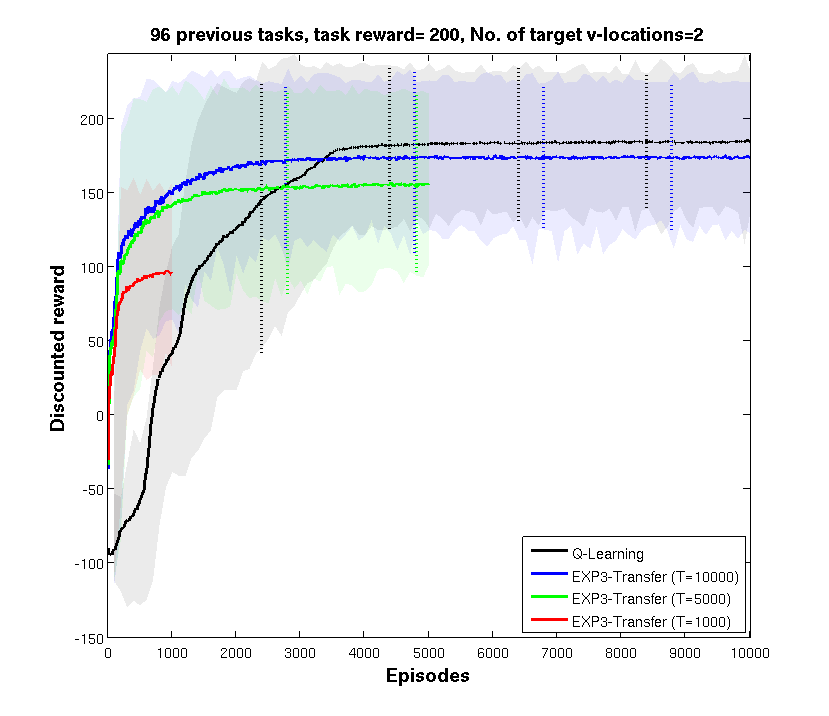
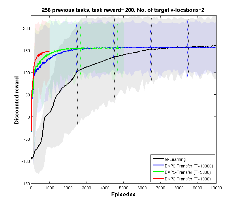
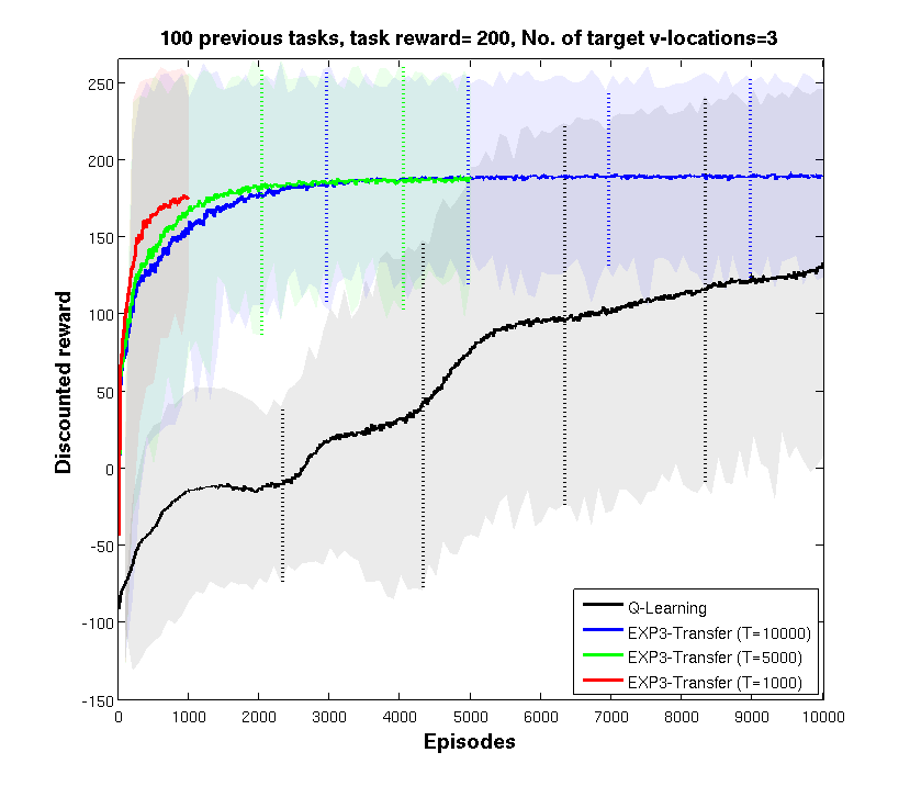
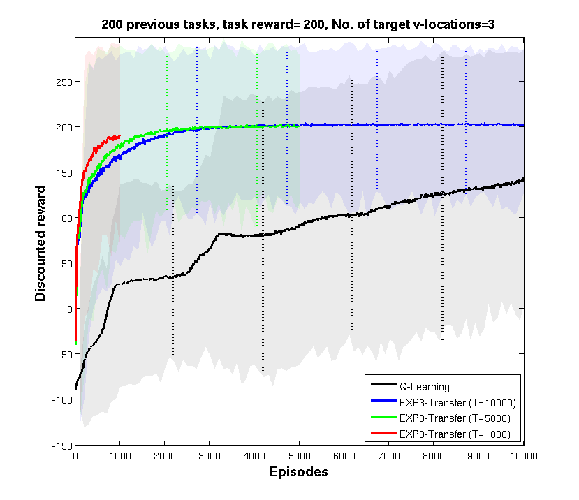
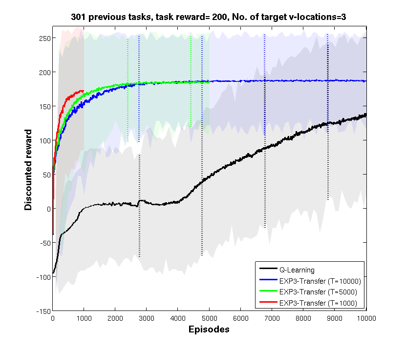
References
- Ammar et al. (2012) Haitham Bou Ammar, Karl Tuyls, Matthew E. Taylor, Kurt Driessen, and Gerhard Weiss. Reinforcement learning transfer via sparse coding. In Proceedings of International Conference on Autonomous Agents and Multiagent Systems, 2012.
- An et al. (2012) Bo An, David Kempe, Christopher Kiekintveld, Eric Shieh, Satinder Singh, Milind Tambe, and Yevgeniy Vorobeychik. Security games with limited surveillance. In Proceedings of the 26th Conference on Artificial Intelligence, 2012.
- Auer et al. (2002a) Peter Auer, Nicolo Cesa-Bianchi, and Paul Fischer. Finite-time analysis of the multiarmed bandit problem. Machine Learning, 47:235–256, 2002a.
- Auer et al. (2002b) Peter Auer, Nicolo Cesa-Bianchi, Yoav Freund, and Robert E. Schapire. The nonstochastic multiarmed bandit problem. SIAM Journal on Computing, 32:48–77, 2002b.
- Azar et al. (2013) Mohammad Gheshlaghi Azar, Alessandro Lazaric, and Emma Brunskill. Regret bounds for reinforcement learning with policy advice. In Proceedings of European Conference on Machine learning (ECML), 2013.
- Baxter (2000) Jonathan Baxter. A model of inductive bias learning. Journal of Artificial Intelligence Research, 12:149–198, March 2000.
- Carroll and Seppi (2005) James L. Carroll and Kevin Seppi. Task similarity measures for transfer in reinforcement learning task libraries. In Proceedings of 2005 IEEE International Joint Conference on Neural Networks, 2005.
- Castro and Precup (2010) Pablo Samuel Castro and Doina Precup. Using bisimulation for policy transfer in mdps. In Proceedings of the the AAAI Conference on Artificial Intelligence, 2010.
- Cesa-Bianchi and Lugosi (2006) Nicolo Cesa-Bianchi and Gabor Lugosi. Prediction Learning and Games. Cambridge University Press, 2006.
- Chickering (2003) David Chickering. Optimal structure identification with greedy search. Journal of Machine Learning Research, 3:507–554, 2003.
- Chickering and Boutilier (2002) David Maxwell Chickering and Craig Boutilier. Learning equivalence classes of bayesian-network structures. Journal of Machine Learning Research, 2:150–157, 2002.
- Dubhashi and Panconesi (2009) Devdatt P. Dubhashi and Alessandro Panconesi. Concentration of Measure Inequalities for the Analysis of Randomized Algorithms. Cambridge University Press, 2009.
- Fernandez et al. (2006) Fernando Fernandez, Javier Garcia, and Manuela Veloso. Probabilistic policy reuse in a reinforcement learning agent. In Proceedings of the 5th International Conference on Autonomous Agents and Multiagent Systems, 2006.
- Fernandez et al. (2010) Fernando Fernandez, Javier Garcia, and Manuela Veloso. Probabilistic policy reuse for inter-task transfer learning. Robotics and Autonomous Systems, 58:866–871, 2010.
- Ferns et al. (2004) Norm Ferns, Prakash Panangaden, and Doina Precup. Metrics for finite markov decision processes. In Proceedings of the Conference on Uncertainty in Artificial Intelligence, 2004.
- Ferrante et al. (2008) Eliseo Ferrante, Alessandro Lazaric, and Marcello Restelli. Transfer of task representation in reinforcement learning using policy-based protovalue functions. In Proceedings of the International Confernce on Autonomous Agent And Multiagent Systems, 2008.
- Hauser et al. (2009) John R. Hauser, Glen L. Urban, Guilherme Liberali, , and Michael Braun. Website morphing. Marketing Science, 28(2):202–223, March 2009.
- Heckerman and Chickering (1995) David Heckerman and David M. Chickering. Learning bayesian networks: The combination of knowledge and statistical data. Machine Learning, pages 20–197, 1995.
- Karp (1972) Richard Karp. Reducibility among combinatorial problems. In Proceedings of a Symposium on the Complexity of Computer Computations, 1972.
- Kirkpatrick et al. (1983) S. Kirkpatrick, C. D. Gelatt, and M. P. Vecchi. Optimization by simulated annealing. Science, 220:671–680, 1983.
- Kolmogorov and Fomin (1970) Andrey Kolmogorov and Sergei V. Fomin. Introductory Real Analysis. Dover Publications, 1970.
- Konidaris and Barto (2007) George Konidaris and Andrew G. Barto. Building portable options: skill transfer in reinforcement learning. In Proceedings of the 20th International Joint Conference on Artificial Intelligence, 2007.
- Lazaric and Restilli (2011) Allesandro Lazaric and Marcello Restilli. Transferring from multiple mdps. In Proceedings of the Neural Information Processing Systems Conference, 2011.
- Lazaric et al. (2008) Allesandro Lazaric, Marcello Restelli, and Andrea Bonarini. Transfer of samples in batch reinforcement learning. In Proceedings of the International Conference on Machine Learning, 2008.
- Levin et al. (2009) David A. Levin, Yuval Peres, and Elizabeth L. Wilmer. Markov Chains and Mixing Times. American Mathematical Society, 2009.
- Littlestone and Warmuth (1994) Nick Littlestone and Manfred K. Warmuth. The weighted majority algorithm. Information and Computation, 108(2):212–261, 1994.
- Locatelli (2000) M. Locatelli. Simulated annealing, algorithms for continuous global optimization: convergence conditions. Journal of Optimization Theory and Applications, 104(1):121–133, 2000.
- Mahadevan (2005) Sridhar Mahadevan. Proto-value functions: Developmental reinforcement learning. In Proceedings of International Conference on Machine Learning, 2005.
- Mitchell and Thrun (1993) Tom M. Mitchell and Sebastian Thrun. Explanation-based neural network learning for robot control. In Adavances in Neural Information Processing Systems, pages 287–294, San Mateo, CA, 1993. Morgan Kaufmann Press.
- Nilim and Ghaoui (2005) Arnab Nilim and Laurent El Ghaoui. Robust control of markov decision processes with uncertain transition matrices. Operations Research, 53(5):780–798, 2005.
- Puterman (1994) Martin L. Puterman. Markov Decision Processes: Discrete Stochastic Dynamic Programming. John Wiley and Sons, 1994.
- Ravindran (2013) Balaraman Ravindran. Relativized hierarchical decomposition of markov decision processes. Decision making: neural and behavioural approaches, 42:465–488, 2013.
- Ravindran and Barto (2003) Balaraman Ravindran and Andrew G. Barto. SMDP homomorphisms: An algebraic approach to astraction in semi-markov decision processes. In Proceedings of the International Joint Conference on Artificial Intelligence, 2003.
- Robert and Casella (2005) Christian P. Robert and George Casella. Monte Carlo Statistical Methods. Springer, Berling, 2005.
- Sorg and Singh (2009) Jonathan Sorg and Satinder Singh. Transfer via soft homomorphisms. In Proceedings of the International Conference on Autonomous Agents and Multiagent Systems, 2009.
- Strehl and Littman (2008) Alexander L. Strehl and Michael L. Littman. An analysis of model-based interval estimation for markov decision processes. Journal of Computer Systems Science, 74(8):1309–1331, 2008.
- Sutton and Barto (1998) Richard S. Sutton and Andrew G. Barto. Reinforcement Learning: An Introduction. MIT Press, Cambridge, MA, 1998.
- Talvitie and Singh (2007) Erik Talvitie and Satinder Singh. An experts algorithm for transfer learning. In Proceedings of the International Joint Conference on Artifical Intelligence, 2007.
- Taylor and Stone (2009) Matthew Taylor and Peter Stone. Transfer learning for reinforcement learning domains: A survey. Journal of Machine Learning Research, 10:1633–1685, 2009.
- Thrun (1996) Sebastian Thrun. Explanation-Based Neural Network Learning: A Lifelong Learning Approach. Kluwer Academic Publishers, Boston, MA, 1996.
- Thrun and Mitchell (1995) Sebastian Thrun and Tom Mitchell. Lifelong robot learning. Robotics and Autonomous Systems, 15:25–46, 1995.
- Vovk (1990) Vladimir Vovk. Aggregating strategies. In Proceedings of the Internation Conference on Computational Learning Theory, 1990.
- Wilson et al. (2007) Aaron Wilson, Alan Fern, Soumya Ray, and Prasad Tadepalli. Multi-task reinforcement learning: A hierarchical bayesian approach. In Proceedings of the International Conference on Learning Theory, 2007.
- Yu and Mannor (2009) Jia Yuan Yu and Shie Mannor. Arbitrarily modulated markov decision processes. In Proceedings of the IEEE Conference on Decision and Control, 2009.
- Yu et al. (2009) Jia Yuan Yu, Shie Mannor, and Nahum Shumkin. Markov decision processes with arbitrary reward processes. Mathematics of Operations Research, 34(3):737–757, 2009.