Numerical Stochastic Perturbation Theory
and the Gradient Flow

Abstract:

We study the Yang-Mills gradient flow using numerical stochastic perturbation theory. As an application of the method we consider the recently proposed gradient flow coupling in the Schrödinger functional for the pure SU(3) gauge theory.

1 The gradient flow coupling

In these Proceedings we focus on the pure SU(3) gauge theory. The Yang-Mills gradient flow $B_{\mu}(t,x)$, $t\geq 0$, is then defined by the flow equation (see [1] for an introduction)

$$\partial_{t}B_{\mu}=D_{\nu}G_{\nu\mu},\quad B_{\mu}|_{t=0}=A_{\mu},$$ (1)

$$G_{\mu\nu}=\partial_{\mu}B_{\nu}-\partial_{\nu}B_{\mu}+[B_{\mu},B_{\nu}],\qquad D_{\mu}=\partial_{\mu}+[B_{\mu},\,\cdot\,],$$ (2)

where $A_{\mu}(x)$ is the fundamental gauge potential integrated over in the functional integral. A key feature of the flow is that correlation functions of the field $B_{\mu}(t,x)$ are automatically finite for flow times $t>0$ once the bare parameters of the theory have been renormalized [2]. Such correlation functions are thus well-defined observables and provide appealing probes for the properties of the theory. One particularly interesting application of the flow is the non-perturbative determination of the running coupling. Through observables at positive flow time one can naturally define a renormalized coupling [1] and compute its scale evolution using step scaling [3].

Consider for example the flow energy density,

$$\big{\langle}E(t)\big{\rangle}=-\frac{1}{2}\,\big{\langle}{\rm Tr}\{G_{\mu\nu}(t)G_{\mu\nu}(t)\}\big{\rangle}.$$ (3)

As shown in [1], a renormalized coupling can be defined in infinite volume as

$$\overline{g}^{2}(\mu)=\frac{(4\pi)^{2}}{3}\big{\langle}t^{2}E(t)\big{\rangle},\quad\mu=1/\sqrt{8t},$$ (4)

where the renormalization scale $\mu$ is set by the flow time. In a finite volume one can analogously define a running coupling by scaling the renormalization scale $\mu$ and all other dimensionful quantities in the system in fixed proportions to the finite spatial extent. Such a definition has been studied in a finite volume with periodic boundary conditions [4], and recently in a box with twisted boundary conditions [5]. Here we are interested in the gradient flow (GF) coupling in a finite volume with Schrödinger functional (SF) boundary conditions, which is defined as [6]

$$\overline{g}^{2}_{\rm GF}(L)\equiv\mathcal{N}^{-1}\langle t^{2}E(t,x_{0})\rangle|_{t=c^{2}L^{2}/8},\quad T=L,\quad x_{0}=T/2,$$ (5)

where $c$ is a constant that relates the flow time to the spatial extent $L$, and $\mathcal{N}$ ensures the correct normalization $\overline{g}^{2}_{\rm GF}=g_{\overline{\rm MS}}^{2}+O(g_{\overline{\rm MS}}^{4})$. The specific scheme in (5) (and so the constant $\mathcal{N}$) in fact depends on the Dirichlet boundary conditions at $x_{0}=0,\,T$, and the values of $c$, $x_{0}$, and $T/L$ one considers. The SF boundary conditions can be chosen such that there is a unique global minimum of the action (up to gauge transformations) around which the perturbative expansion of the coupling is easy to set up [6, 7]. This is indeed crucial for the application we are going to discuss.

In these Proceedings we study the GF coupling in the SF using lattice perturbation theory. From perturbation theory one can extract valuable information for a non-perturbative determination of the running coupling. First of all, the matching to other schemes is generally done at high energies using perturbation theory. Secondly, cutoff effects in the step-scaling function can be determined perturbatively and be used to improve non-perturbative data [8]. In order to make these determinations more effective, however, perturbation theory needs to be pushed beyond the 1-loop order, which is in most cases technically involved. Although codes have been developed for the automation of such calculations [9], the inclusion of the gradient flow and the need for high order contributions complicate things further, rendering these computations rather challenging. For this reason we rely on Numerical Stochastic Perturbation Theory (NSPT) (see [10] for an introduction). Due to the similarities between the Langevin and gradient flow equations, NSPT is a natural framework for a perturbative numerical solution of the flow. In the next section we start with a reminder of the lattice setup as discussed in [6]. We then recall the basics of NSPT and explain how the gradient flow equation can be solved in this framework. Finally, we present our results for the flow energy density $E$ to 3-loops in perturbation theory which gives direct access to $\overline{g}^{2}_{\rm GF}$ at 2-loops.

2 The gradient flow coupling on the lattice

The gradient flow equation (1) can be studied on the lattice by introducing the field $V_{\mu}(t,x)$ (also known as “Wilson flow” [1]) defined by the equation

$${\partial_{t}}{V}_{\mu}(t,x)=-\big{\{}g_{0}^{2}\nabla_{x\mu}S_{W}({V}(t))\big{\}}{V}_{\mu}(t,x),\quad V_{\mu}(0,x)=U_{\mu}(x),$$ (6)

where $\nabla_{x\mu}$ is the Lie-derivative with respect to $V_{\mu}(t,x)$, and $S_{W}$ is the Wilson plaquette action. Analogously, we choose the Wilson plaquette action also for the gauge field $U_{\mu}(x)$. Following [6], we then consider an $(L/a)^{4}$ lattice and impose, for all values $t\geq 0$ of the flow time, the SF boundary conditions:

$$V_{\mu}(t,x+\hat{k}L)=V_{\mu}(t,x),\quad V_{k}(t,x)|_{x_{0}=0,\,L}=\mathds{1}.$$ (7)

Given these boundary conditions, the action $S_{W}$ has a unique global minimum (up to gauge transformations) corresponding to the field configuration $\mathcal{V}_{\mu}(x)=\mathds{1}$, $\forall x,\mu$. Finally, we define the energy density $E$ on the lattice through the continuum formula (3) and the lattice definition of the field strength tensor $G_{\mu\nu}$ given in [1]. In fact, as noticed in [6], a renormalized coupling can be defined as in (5) considering only the spatial or temporal components of the strength tensor in the expression for $E$. Later, we will refer to the corresponding contributions as $E_{s}$ and $E_{t}$, respectively.

3 A numerical perturbative solution for the gradient flow

The idea of NSPT is to solve the equations of stochastic perturbation theory numerically [11]. One starts from the stochastic quantization of the lattice theory, where the fundamental fields evolve in the extra coordinate $t_{s}$ (known as stochastic time) according to the Langevin equation

$${\partial_{t_{s}}}U_{\mu}(t_{s},x)=-\big{\{}\nabla_{x\mu}S_{W}(U(t_{s}))+\eta_{\mu}(t_{s},x)\big{\}}U_{\mu}(t_{s},x),$$ (8)

where $\eta_{\mu}(t_{s},x)$ is a Gaussian distributed noise field. The Langevin equation is then discretized in the stochastic time, $t_{s}=n\varepsilon_{s}$, and a general solution is obtained according to a given integration scheme e.g. Runge-Kutta. Last, introducing in the solution the perturbative expansion

$$U_{\mu}(t_{s},x)\to\sum_{k}g_{0}^{k}\,U^{(k)}_{\mu}(t_{s},x),\quad U^{(0)}_{\mu}(t_{s},x)\equiv\mathcal{V}_{\mu}(x),$$ (9)

where $\mathcal{V}$ is the field configuration around which we expand, the result is a hierarchy of equations that can be truncated consistently and solved numerically. In the limit of $t_{s}\to\infty$ the noise average of any observable $\mathcal{O}$ evaluated on the perturbative solution (9) is then expected to converge order-by-order in perturbation theory to the corresponding expectation value of the lattice theory, i.e.

$$\lim_{t_{s}\to\infty}\big{\langle}{\mathcal{O}\big{[}\sum_{k}g_{0}^{k}\,U^{(k)}(t_{s})\big{]}}\big{\rangle}_{\eta}=\lim_{t_{s}\to\infty}\sum_{k}\,g_{0}^{k}\,\langle{\mathcal{O}}^{(k)}(t_{s})\rangle_{\eta}=\sum_{k}\,g_{0}^{k}\,\mathcal{O}_{k},$$ (10)

where $\langle\cdots\rangle_{\eta}$ is the average over the noise field distribution, and $\mathcal{O}_{k}$ is the $k$-th order coefficient of the perturbative expansion of $\langle\mathcal{O}\rangle$. The gradient flow can now be included as follows. Compared to the Langevin equation, there are two important differences to consider: in the flow equation the noise term is absent, and the initial distribution of the gauge field $U_{\mu}(x)$ (here given by a perturbative expansion of the Langevin equation) has to be taken into account (cf. (6)). To this end, we introduce in a discrete solution of the flow equation

$${V}_{\mu}(t_{s};t,x)\to\sum_{k}g_{0}^{k}\,{V}^{(k)}_{\mu}(t_{s};t,x),\quad V^{(k)}_{\mu}(t_{s};0,x)=U^{(k)}_{\mu}(t_{s},x),\quad\forall k,$$ (11)

where $t=n\varepsilon$, and $V_{\mu}(t_{s};t,x)$ inherits the $t_{s}$ dependence from the initial condition. The result of the expansion is the same hierarchy of equations as for the Langevin equation, except that the noise field is set to zero. For a given initial gauge field configuration, the flow equation can thus be integrated numerically up to the desired flow time, order-by-order, using the same techniques. In particular, note that the flow field (11) is a function of the gauge field (9) through the initial condition. The perturbative expansion of any flow observable is then obtained as in (10).

To conclude, both perturbative solutions of the Langevin and flow equations are derived from a discrete approximation of these equations. Results have then to be extrapolated for $\varepsilon_{s},\varepsilon\to 0$ in order to eliminate the effects of the discretization. In addition, in NSPT stochastic gauge fixing is fundamental to obtain sensible results [10]. We refer however to [12] for a detailed discussion of stochastic gauge fixing in NSPT for SF schemes.

4 Results

4.1 Determination of $\mathcal{N}$ and comparison with analytical results

As discussed before, a renormalized coupling can be defined considering the separate contributions

$${\mathcal{E}}_{i}\equiv\langle t^{2}E_{i}(t,L/2)\rangle=\mathcal{N}_{i}\,g_{0}^{2}+{\mathcal{E}}_{i}^{(1)}\,g_{0}^{4}+{\mathcal{E}}_{i}^{(2)}\,g_{0}^{6}+\ldots,\quad i=s,\,t,$$ (12)

where the lowest-order coefficient $\mathcal{N}$ enters as part of the definition of the coupling (we leave out the subscript $i$ when a statement holds for both $s$ and $t$). This term has been computed in [6] for the lattice setup we are considering. As a first result we reproduced the values of $\mathcal{N}$ for lattices up to $L/a=12$, and different choices of $c$ (cf. 5). Some examples are collected in fig. 1. The data are extrapolated in $\epsilon^{2}$ since a second-order integrator was used for both the Langevin and flow equation and we took $\varepsilon_{s}=\varepsilon$. In particular, we considered a linear fit to all data points and a constant fit to the data omitting $\varepsilon=0.05$, and estimated systematic effects as the difference between the two fits. The extrapolated values agree within errors with the analytical results.

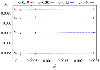
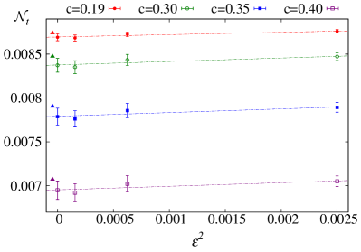
Figure 1: Extrapolations of $\mathcal{N}$ to zero step-size for $L/a=12$ and several schemes $c$. Left: Values for the spatial contribution $\mathcal{N}_{s}$. Right: Values for the temporal contribution $\mathcal{N}_{t}$. Analytical results are depicted as triangles.

4.2 Determination of $\mathcal{E}^{(1)}$ and comparison with Monte Carlo data

Next, we consider the NLO contribution given by $\mathcal{E}^{(1)}$. For this quantity no independent determinations are available for direct comparison. Hence, as a crosscheck on our results, we obtained an estimation of $\mathcal{E}^{(1)}$ from Monte Carlo (MC) simulations. We performed pure SU(3) gauge simulations at 12 values of $\beta=6/g_{0}^{2}\in[50,1200]$ at fixed $L/a$, and we extracted $\mathcal{E}^{(1)}$ from a fit of $\mathcal{E}$ to (12) fixing $\mathcal{N}$ to its analytical value. The results we obtained for $L/a=8$ are summarized in Table 1. The agreement between NSPT and MC simulations is generally good (max deviation $\sim 2.6\,\sigma$), and we note NSPT to be systematically more precise at a comparable computational cost.

	$\mathcal{E}^{(1)}_{s}$			$\mathcal{E}^{(1)}_{t}$
$c$	MC	NSPT		MC	NSPT
0.19	0.00478 (09)	0.00463 (2)		0.00486 (09)	0.00461 (2)
0.30	0.00552 (15)	0.00546 (5)		0.00557 (17)	0.00541 (5)
0.40	0.00483 (18)	0.00478 (6)		0.00479 (22)	0.00472 (7)
0.50	0.00355 (14)	0.00349 (6)		0.00351 (21)	0.00350 (6)

Table 1: Comparison between Monte Carlo and NSPT results for $\mathcal{E}^{(1)}$ for an $L/a=8$ lattice and different values of $c$. The spatial $\mathcal{E}^{(1)}_{s}$ and the temporal contribution $\mathcal{E}^{(1)}_{t}$ are shown.

4.3 Determination of $\mathcal{E}^{(2)}$

The highest order we have computed is the NNLO contribution $\mathcal{E}^{(2)}$. An example of the $\varepsilon\to 0$ extrapolation for an $L/a=8$ lattice is shown in fig. 2. The results of the extrapolations have been compared with the ones obtained by MC simulations. Although agreement was found, the errors on the extracted values for $\mathcal{E}^{(2)}$ from MC simulations were quite large (about 20-50%), thus providing not such a stringent constraint on our determination. Smaller values of $\beta$ have probably to be considered in order to resolve this contribution from the MC data. The results obtained from NSPT however have a good overall precision of $\sim 1\%$ for this small lattice size.

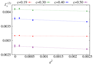
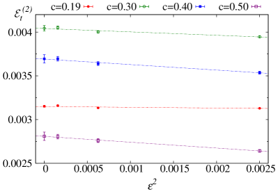
Figure 2: Extrapolations of $\mathcal{E}^{(2)}$ to zero step-size for $L/a=8$ and several schemes $c$. Left: Values for the spatial contribution $\mathcal{E}^{(2)}_{s}$. Right: Values for the temporal contribution $\mathcal{E}^{(2)}_{t}$.

4.4 Relative variance and autocorrelations

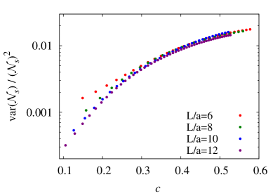
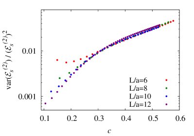
Figure 3: Relative variance as a function of $c$ for different $L/a$ for computations at $\varepsilon=0.0125$.

Finally, we present some results on the variance of $\mathcal{E}_{s}$ (analogous results hold for $\mathcal{E}_{t}$). More precisely, in fig. 3 we show the relative variance of $\mathcal{N}_{s}$ and $\mathcal{E}^{(2)}_{s}$ as a function of $c$ for different lattice sizes $L/a$. Here we consider only computations with $\varepsilon=0.0125$ which are the most expensive ones we performed. The first observation is that the relative variance is rather independent of $L/a$ for schemes with $c\gtrsim 0.3$. Secondly, higher order terms have relative variance comparable to the lowest ones, indicating that a similar level of precision can be reached. Note in particular that the results in fig. 3 give direct information on the number of independent measurements necessary to obtain a certain precision on the result. For example, to compute $\mathcal{N}_{s}$ for $c\sim 0.3$ at the 0.1% level we need $\sim 5000$ independent measurements, for $\mathcal{E}_{s}^{(2)}$ instead $\sim 9000$ are necessary. The level of precision on $\overline{g}^{2}_{\rm GF}$ one can achieve then seems relatively good with moderate statistics. To conclude, one has to consider that in order to obtain $\mathcal{E}^{(k)}$ for a given scheme $c$ at a certain level of precision, the cost of the computation scales $\propto(L/a)^{6}$. Apart from the volume factor $\propto(L/a)^{4}$, the cost of integrating the flow increases $\propto(L/a)^{2}$ for fixed $c$ (cf. (5)). Autocorrelations also increase $\propto(L/a)^{2}$ as expected for the Langevin dynamics. The measurement frequency of the flow along the stochastic time then can be scaled $\propto(L/a)^{-2}$ without significant loss in the statistical precision of the determination.

5 Conclusions & outlook

We studied the flow energy density $E$ in the SF at 3-loops in perturbation theory for the pure SU(3) gauge theory. We reproduced the values for $\mathcal{N}$ in [6] and compared higher orders to MC results finding good agreement. Our study shows that a precise determination of $\overline{g}^{2}_{\rm GF}$ using NSPT is feasible with moderate statistics. As a next step we plan to investigate the GF coupling in QCD. Larger lattice sizes will be considered in order to extrapolate the matching coefficients to other schemes, and the corresponding cutoff effects in the step-scaling function will be determined.

References

- [1] M. Lüscher, Properties and uses of the Wilson flow in lattice QCD, JHEP 1008 (2010) 071, [arXiv:1006.4518].
- [2] M. Lüscher and P. Weisz, Perturbative analysis of the gradient flow in non-abelian gauge theories, JHEP 1102 (2011) 051, [arXiv:1101.0963].
- [3] M. Lüscher, P. Weisz, and U. Wolff, A numerical method to compute the running coupling in asymptotically free theories, Nucl.Phys. B359 (1991) 221–243.
- [4] Z. Fodor, K. Holland, J. Kuti, D. Nogradi, and C. H. Wong, The Yang-Mills gradient flow in finite volume, JHEP 1211 (2012) 007, [arXiv:1208.1051].
- [5] A. Ramos, The gradient flow in a twisted box, arXiv:1308.4558.
- [6] P. Fritzsch and A. Ramos, The gradient flow coupling in the Schrödinger functional, JHEP 1310 (2013) 008, [arXiv:1301.4388].
- [7] M. Lüscher, R. Narayanan, P. Weisz, and U. Wolff, The Schrödinger functional: a renormalizable probe for non-abelian gauge theories, Nucl.Phys. B384 (1992) 168–228, [hep-lat/9207009].
- [8] G. de Divitiis et al., Universality and the approach to the continuum limit in lattice gauge theory, Nucl.Phys. B437 (1995) 447–470, [hep-lat/9411017].
- [9] D. Hesse and R. Sommer, A one-loop study of matching conditions for static-light flavor currents, JHEP 1302 (2013) 115, [arXiv:1211.0866].
- [10] F. Di Renzo and L. Scorzato, Numerical stochastic perturbation theory for full QCD, JHEP 0410 (2004) 073, [hep-lat/0410010].
- [11] F. Di Renzo, G. Marchesini, P. Marenzoni, and E. Onofri, Lattice perturbation theory on the computer, Nucl.Phys.Proc.Suppl. 34 (1994) 795–798.
- [12] M. Brambilla, M. Dalla Brida, D. Hesse, F. Di Renzo, and S. Sint, Numerical Stochastic Perturbation Thoery for Schrödinger Functional schemes, PoS LATTICE2013 (2013) 325.