Comparing the WFC3 IR Grism Stare and Spatial-scan Observations for Exoplanet Characterization

Abstract

We report on a detailed study of the measurement stability for WFC3 IR grism stare and spatial scan observations. The excess measurement noise for both modes is established by comparing the observed and theoretical measurement uncertainties. We find that the stare-mode observations produce differential measurements that are consistent and achieve $\sim 1.3$ times photon-limited measurement precision. In contrast, the spatial-scan mode observations produce measurements which are inconsistent, non-Gaussian, and have higher excess noise corresponding to $\sim 2$ times the photon-limited precision. The inferior quality of the spatial scan observations is due to spatial-temporal variability in the detector performance which we measure and map. The non-Gaussian nature of spatial scan measurements makes the use of $\chi^{2}$ and the determination of formal confidence intervals problematic and thus renders the comparison of spatial scan data with theoretical models or other measurements difficult. With better measurement stability and no evidence for non-Gaussianity, stare mode observations offer a significant advantage for characterizing transiting exoplanet systems.

1 Introduction

The objective of this paper is to characterize the measurement stability of stare and spatial scan mode observations that have been used to study exoplanets with WFC3. Because the spatial scan mode moves the spectrum over a large range of detector pixels, which potentially have different properties, it is important to test the measurement stability as a function of location on the array. Exoplanet spectroscopy via the transit method typically relies on taking the difference of two large numbers to measure a small number. This approach makes knowledge of measurement systematic errors critically important. For characterizing an exoplanet’s terminator transmission spectrum (using the primary eclipse event) or dayside emission spectrum (using the secondary eclipse event), the typical spectroscopic measurement dynamic range varies from between $\sim$1000:1 (1000 ppm) in the mid-infrared to $\sim$20,000:1 (50 ppm) in the visible and near-infrared. Continuing to improve the measurement dynamic range is a priority. Because higher precision enables new science such as the detection of new opacity sources, improved abundance constraints, ingress/egress light curve mapping, measurement of atmospheric temporal variability, and characterization of smaller targets, pushing for higher precision is critically important to the field. Most of the instruments used for transit spectroscopy today were not specifically designed for the task; this makes characterization of these instruments an especially important activity.

Due to a combination of space-based location, good wavelength coverage, moderate spectral resolution, and excellent telescope pointing, the best instrument available today for transit spectroscopy is arguably WFC3 using the IR grism. The instrument has already been used extensively for exoplanet spectroscopy (Berta et al. 2012, Swain et al. 2013, Huitson et al. 2013, Wakeford et al. 2013, Deming, et al. 2013, Mandell et al. 2013, Stevenson et al. 2013), and the field of exoplanet atmospheric characterization is beginning to rely on this critical community resource with programs conducted using both stare and spatial scan observational modes. Although a detailed comparison of these modes did not previously exist, the instrument status report (ISR) describing the spatial scan mode does note photometric ‘flicker’ (McCullough & MacKenty 2012) at the 3% level in spatial scan mode testing which raises questions about how the mode will perform for spectrophotometry measurements. Motivated by the growing importance of this instrument, we undertook a detailed analysis in which we determined the measurement stability for differential spectroscopy, the approach often used to characterize the atmospheres of transiting planets. WFC3 is an exceptional instrument that has produced extraordinary measurements. Our findings, reported below, should be viewed in the context of the astronomer’s desire to operate an instrument well beyond the original engineering design space. Our approach to characterizing the instrument is simple. Absent an absolute calibration reference, the only way to assess instrument stability is to make the same measurement many times and quantify the repeatability.

2 Methods

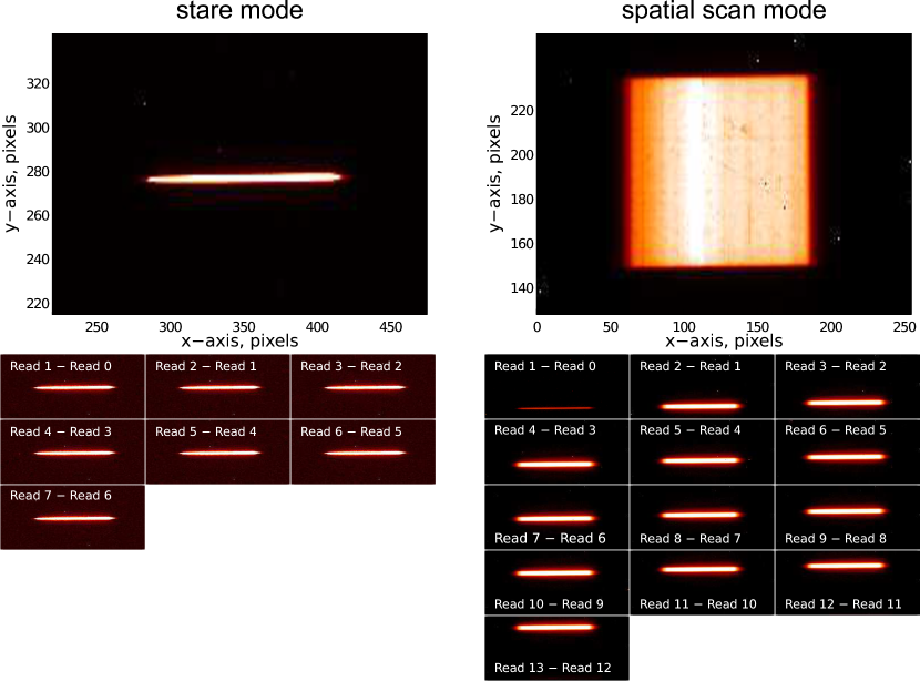
Figure 1: An illustration of the difference between stare-mode observations (left), in which the spacecraft pointing is fixed in inertial space, and spatial-scan observations (right) in which the spacecraft is scanned in a direction perpendicular to the grism dispersion axis. The top figures are the respective images from a single integration consisting of a series of sample-up-the-ramp nondestructive reads. The lower figures show the difference between consecutive nondestructive reads. The stare observations have fewer nondestructive reads (Nsamp=8) than the spatial scan observations (Nsamp=14) shown here. The target of these observations is GJ 1214.

To quantify the stability of the WFC3 spectrophotometric time series observations, we measure differences between portions of the time series and determine how the observed noise compares to the theoretically expected noise. Ideally, we would quantify the stability using measurements of calibration targets with carefully selected properties. This could potentially require tens of Hubble orbits, and no such calibration program has been carried out for WFC3 IR grism spectroscopy. An alternative approach is to base the analysis on a science data set, preferably one where the same object has been repeatedly observed in the same mode. Fortunately, such a target exists; the GJ 1214 exoplanet host star has been observed extensively with the WFC3 IR grism using both stare and spatial scan mode observations, and we use these data for our study. For all of the observations we analyzed, the GJ 1214 system was observed with 4 consecutive HST orbits timed to place 2 orbits before the primary eclipse event and one orbit after the primary eclipse event. In our analysis, the first orbit is excluded to allow for spacecraft settling and detector effects that could uniquely affect the first orbit. We analyze the difference between the pre- and post-eclipse time series in which no exoplanet-related event impacts the measurement. The differential measurement stability is characterized using the mean and the variance.

All infrared observations with WFC3 are conducted in MULTIACCUM mode which starts with two array resets, followed quickly by an initial readout, and then a user selectable number of nondestructive reads, specified by the MULTIACCUM mode and the Nsamp parameter (see WFC3 handbook). The non-destructive reads (Nsamp=1 to Nsamp=N) sample up the ramp as the detector accumulates electrons. The initial readout after a detector reset, termed the ”zero read” (Nsamp=0), measures the reset pedestal. The light measured during a single integration is the total number of photoelectrons measured during the sample up the ramp. For WFC3, all detector reads, including the zero read, are saved and available for download from the MAST archive. GJ 1214b data was executed using both stare and scan observing modes (see Figure 1 and Table 1) and in all cases, the detector was operated with the same integration and number of nondestructive reads (Nsamp value) for each of the four-orbit sequences. In stare mode, the spectrum is held at the same location and stabilized at the subpixel level on the detector by the HST pointing system. The stare mode has frequently been used for exoplanet spectroscopy because it minimizes sensitivity to inter and intra-pixel non-uniformity. Recently, the spatial scan mode has been developed for WFC3 (McCullough & MacKenty 2012) to improve instrument duty cycle and bright target capability. In this mode, the spectrum is scanned across the detector in the spatial direction during an integration; this process is then repeated in the same detector location for subsequent integrations.

We measure instrument stability by constructing a quantity that should be zero and tracking the behavior of this quantity. Our merit figure for instrument stability is the difference of the measured spectrum before eclipse and after eclipse. Subject to the assumption that the star is constant, this difference should be zero; departures from zero represent changes in the instrument spectral transfer function. Any deviations from zero, whatever the origin, represent aspects of the measurement that must be accounted for when estimating the measurement precision. To maintain sensitivity to array location-dependent effects, we extract the electrons measured during each sample up the ramp read. We do this by using the $*$_raw.fits data-type files, which are the most minimally processed files available for WFC3.

We begin the analysis by constructing a set of difference images, $\Delta I$, which isolate the photoelectrons detected during a single sample up the ramp read by taking the difference of consecutive nondestructive reads,

$$\Delta I_{i}=I_{i}-I_{i-1},$$ (1)

where $I$ is a single detector read image, and has time-related indices corresponding to orbit, $o$, integration, $j$, and sample up the ramp read, $i$. This subtraction also removes array artifacts and the background associated with previous reads. The $\Delta I_{i}$ images contain the spectrum + background measured during a specific nondestructive read. For each $\Delta I_{i}$ image (see Figure 1), we determine the spectrum and background location, subtract the background, and collapse the spectrum along the spatial axis. The result is a spectrum, $F_{t}(\lambda)$, where $t$ can be decomposed with indices representing orbit, $o$, integration number, $j$, and sample up the ramp read number, $i$. To measure the achieved stability, we take the coupled difference $\Delta F_{i,j}(\lambda)$ of spectra measured in the pre and post eclipse Hubble orbit:

$$\Delta F_{i,j}(\lambda)=F_{pre,i,j}(\lambda)-F_{post,i,j}(\lambda),$$ (2)

i.e. the first read of the first exposure of the pre-eclipse orbit is subtracted from the first read of the first exposure of the post eclipse orbit, etc. (see Figure 2). Taking the coupled difference has the effect of removing the repeatable effects within an orbit, like a ramp buildup. We then construct an average quantity that removes the dependence on integration, index $j$,

$$\Delta S_{i}(\lambda)=\frac{\langle\Delta F_{i,j}(\lambda)\rangle}{\langle F_{pre,i,j}(\lambda),F_{post,i,j}(\lambda)\rangle}.$$ (3)

The quantity $\Delta S_{i}(\lambda)$ measures the normalized difference between spectra in orbits on either side of eclipse and is a merit figure for spectral measurement stability. Ideally, it should be zero; departures from zero indicate that the instrument spectral transfer function has changed. For each of the $\Delta S_{i}(\lambda)$, we determine the variance

$$\sigma^{2}_{\Delta S_{i}}=VAR\left[\frac{\Delta F_{i,j}(\lambda)}{\langle F_{pre,i,j}(\lambda),F_{post,i,j}(\lambda)}\right]_{j},$$ (4)

where VAR is the variance taken over the set of $j$ integrations. We also calculate the average of the $\Delta S_{i}(\lambda)$, which removes the dependence on the integration index, $i$,

$$\Delta S(\lambda)=\langle\Delta S_{i}(\lambda)\rangle,$$ (5)

where the variance of $\Delta S(\lambda)$ is given by,

$$\sigma^{2}_{\Delta S}=VAR[\Delta S_{i}(\lambda)]_{i},$$ (6)

and where VAR is the variance taken over the set of $i$ sample-up-the-ramp reads. We also calculate the photon noise for the observations as,

$$\sigma^{2}_{phot}=N_{pre}+N_{post},$$ (7)

where $N$ is the number of photons, and add additional noise for the measurement noise due to the read process and the background. By comparing the photon noise (i.e., the theoretical limit) to the measured noise, we determine the excess noise in the system.

For the spatial scan observations we analyzed, the reads are evenly spaced in time after read 1. Thus for the spatial-scan observations with Nsamp=14 or 16, there are 14 or 16 nondestructive reads (including the zero read), and in our analysis we use the difference between reads $i$ and $i-1$ from read 2 through 13 or 15, which corresponds to a set of 12 or 14 independent measurements, [$\Delta S_{2}(\lambda)$…$\Delta S_{13}(\lambda)$], which can be used to study measurement repeatability. The observations conducted in stare mode have 8 samples up the ramp and the integration time is identical starting from the zero read. For those observations, we construct 7 independent measurements. If the measurements are repeatable, $\Delta S_{i}(\lambda)=\Delta S_{k}(\lambda)$, where $i$ and $k$ indicate different sample-up-the-ramp reads.

Table 1: Data used in this analysis.

visit	date	mode	Nsamp	scan length	integrations	integration
				(pixels)	per orbit	time (s)
stare visit 1	9-Oct-10	RAPID	8	NA	48	5.971
stare visit 2	28-Mar-11	RAPID	8	NA	48	5.971
stare visit 3	23-Jul-11	RAPID	8	NA	48	5.971
scan visit 1	27-Sep-12	SPARS10	14	80.76	17	88.436
scan visit 2	3-Oct-12	SPARS10	14	80.72	17	88.436
scan visit 3	11-Oct-12	SPARS10	14	80.66	17	88.436
scan visit 4	19-Oct-12	SPARS10	14	80.94	17	88.436
scan visit 5	29-Jan-13	SPARS10	14	81.22	17	88.436
scan visit 6	13-Mar-13	SPARS10	16	104.45	19	103.129
scan visit 7	15-Mar-13	SPARS10	16	104.87	19	103.129
scan visit 8	27-Mar-13	SPARS10	16	104.76	19	103.129
scan visit 9	4-Apr-13	SPARS10	16	104.95	19	103.129
scan visit 10	12-Apr-13	SPARS10	16	104.66	19	103.129
scan visit 11	1-May-13	SPARS10	16	104.60	19	103.129
scan visit 12	6-Jul-13	SPARS10	16	104.48	19	103.129
scan visit 13	4-Aug-13	SPARS10	16	104.24	19	103.129
scan visit 14	20-Aug-13	SPARS10	16	104.38	19	103.129

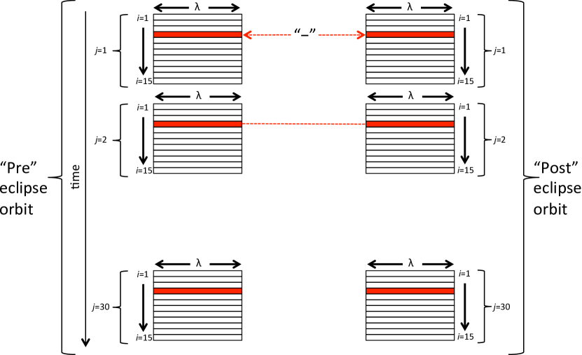
Figure 2: Diagram of data/index relationships illustrating how $\Delta S_{i}(\lambda)$ is constructed. The red regions represent the data used in the equation above to construct $\Delta S_{4}(\lambda)$.

3 Results

We investigated the excess noise and repeatability using the $\Delta S_{i}$ and its statistics for a range of spectral resolutions by averaging in the spectral direction. These results are summarized for single and multiple visits in Table 2 and Figure 3. For the stare mode, we find a relatively small amount of excess noise compared to the photon noise and consistent $\Delta S_{i}$ measurements $(\Delta S_{i}\approx\Delta S_{k})$. However, the spatial-scan mode observations show significant excess noise and that $\Delta S_{i}\neq\Delta S_{k}$ in the majority of cases, indicating the measurements are not repeatable. We tested the visit-to-visit repeatability of the measurement by comparing the visit-averaged $\Delta S$ and found that the repeatability is significantly better in stare mode than for spatial scan mode, where we find significant visit-to-visit variations (right panel of Figure 3).

Table 2: Summary of findings for stare and spatial-scan modes.

Observing mode	Condition	Comment
stare	$\sigma_{\Delta S_{i}}\approx\sigma_{photon}$	Approaches theoretical noise limit $\sim 1.25\times$ photon noise
	$\Delta S_{i}\approx\Delta S_{k}$	Measurements repeatable
	$\Delta S_{i}$ Gaussian	interpretation straightforward
spatial scan	$\delta_{\Delta S_{i}}>\delta_{photon}$	Significant excess noise, up to more than $2\times$ photon noise
	$\Delta S_{i}\neq\Delta S_{k}$	Measurements not repeatable
	$\Delta S_{i}$ non-Gaussian	science interpretation problematic

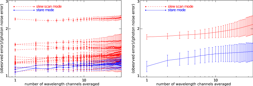
Figure 3: Excess noise for stare and spatial-scan modes as a function of spectral averaging for individual visits (left) and the multivisit average (right). The 1 $\sigma$ error bars indicate the differences observed when repeating the analysis for different wavelengths in the spectrum covering 1.15 to 1.65 $\mu$m.

In addition to analyzing the variance of $\Delta S_{i}$, we also analyzed its statistical properties. Given an unbiased source of noise, we expect the $\Delta S_{i}$ measurements to follow a normal distribution around the mean, $\Delta S$. We analyzed the stare and spatial scanning observations using a set of statistical tests, including the $\chi^{2}$, Kolmogorov-Smirnov, Shapiro-Wilk, Anderson-Darling, and D’Agostino-Pearson tests. Each test generates a statistic and an associated $p$-value. While the range and meaning of each test’s calculated statistic varies, the $p$-value provides a consistent way to interpret results across tests. The $p$-value is the probability of observing the given data values under the assumption that the null hypothesis (here, of Gaussianity) is true. A low $p$-value provides evidence that the null hypothesis may not apply to the observed data; e.g., a $p$-value of 0.04 indicates that the null hypothesis can be rejected at the 95% confidence level, because it is less than 0.05.

The $\chi^{2}$ test compares two distributions represented as discrete histograms, so the choice of histogram granularity can influence the results. We used 10 bins in all $\chi^{2}$ tests and compared the observed frequencies to those expected from a random variable with a Gaussian distribution having the same mean and standard deviation as the observed data.

The tests were conducted on the measured $\Delta S_{i}$ spectra for a given visit at 1.10 to 1.65 $\mu$m. For the spatial-scan mode, observations for all reads were combined. We also tested the collection of all observations across all visits for each mode (stare and spatial scan). The $p$-values for the stare mode data, across all tests, are consistently too high for us to reject the Gaussian hypothesis (see Table 3, “all stare”). In contrast, the Gaussian hypothesis is strongly rejected for the spatial-scan mode data, by all tests, with $>99$% confidence (see Table 3, “all scan”). We also examined the data from each visit individually. For the stare mode, the Gaussian hypothesis once again cannot be rejected with confidence for any visit. However, for the spatial-scan mode, the Gaussian hypothesis is rejected with 99% confidence for the majority of the visits (2-6, 8, 9, 11, 13, and 14). ). The remaining four visits (1, 7, 10, and 12) do not have sufficient evidence to reject the Gaussian hypothesis with 99% confidence, given the number of observations available in each spatial scan visit. Yet even in cases for which noise may be normally distributed during a given visit, the noise is not consistent across visits, implying that quantities estimated by averaging data from multiple visits have an uncertainty that does not decrease as the square root of the number of visits.

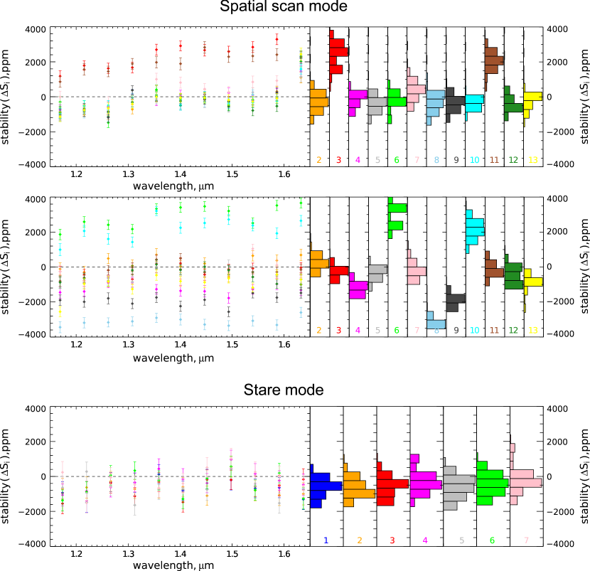
Figure 4: Three examples showing that observations are not repeatable in spatial scan mode (scan mode visit 4 top and visit 5 middle) whilst being repeatable in stare mode (bottom). Shown to the left are the orbit averaged pre-post spectra for individual detector reads with the histograms for individual detector reads shown to the right; ideally, all measurements would be zero within the errors and the departures from zero here are due to systematic errors. The average values of individual detector reads, corresponding to measurements made seconds apart, can easily disagree at the level of $\sim 2000$ ppm (left) and by several standard deviations using the spatial-scan mode. Stare observations (right) are much more repeatable.

Table 3: P-values for Gaussianity tests applied to stare and spatial scan data.

visit	$\chi^{2}$	Kolmogorov-	Sharipo-	Anderson-	D’Agostino-
		Smirnov	Wilk	Darling	Pearson
stare visit 1	0.39	0.83	0.85	$>0.15$	0.91
stare visit 2	0.54	0.88	0.85	$>0.15$	0.71
stare visit 3	0.84	0.77	0.71	$>0.15$	0.29
all stare	0.99	0.98	0.97	$>$0.15	0.58
scan visit 1	0.08	0.55	0.05	$>0.05$	0.17
scan visit 2	2e-15	5e-4	5e-10	$<0.01$	3e-11
scan visit 3	3e-4	0.05	4e-5	$<0.01$	1e-3
scan visit 4	6e-13	5e-5	6e-9	$<0.01$	9e-8
scan visit 5	9e-8	0.01	3e-5	$<0.01$	0.02
scan visit 6	7e-13	0.02	6e-7	$<0.01$	7e-8
scan visit 7	0.35	0.41	0.03	$>0.05$	0.03
scan visit 8	8e-11	0.10	1e-5	$<0.01$	1e-4
scan visit 9	0.01	0.23	2e-3	$<0.01$	7e-4
scan visit 10	0.31	0.88	0.35	$>0.15$	0.89
scan visit 11	2e-5	0.04	2e-5	$<0.01$	5e-5
scan visit 12	0.96	0.66	0.62	$>0.15$	0.49
scan visit 13	2e-8	0.06	2e-6	$<0.01$	7e-8
scan visit 14	6e-35	3e-4	2e-11	$<0.01$	5e-12
all scan	0.00	0.00	2e-31	$<$0.01	3e-55

4 Discussion

The non-Gaussian nature of the spatial-scan data makes estimation of statistical significance problematic as normal Gaussian statistics cannot be assumed. The departures from Gaussianity become even stronger when multiple spatial-scan visits are combined. The finding that the spatial scan measurement variance decreases more slowly than $1/N$ (where $N$ is the number of measurements) indicates that the individual measurements are not fully statistically independent. This combination of non-Gaussanity and a lack of statistical independence has three important implications for measurements of exoplanets using the spatial scan mode.

1. Comparison of a spatial scan result with other measurements becomes problematic because the confidence interval is no longer well defined. We can measure the standard deviation, but without knowledge of the underlying distribution, we cannot know what the statistical significance of the result is. This has direct relevance to the comparison of results obtained with WFC3 spatial-scan measurements of XO-1b (Deming et al. 2013) and previous stare-mode observations with NICMOS (Tinetti et al. 2010). If the spatial-scan measurements of XO-1b exhibit non-Gaussian properties similar to those of the spatial-scan data sets we analyzed, the formal confidence of the statistical comparison reported by Deming et al. (2013) likely requires revision.

2. Increasing measurement precision by repeated spatial-scan observations is observationally expensive because the measurement variance does not decrease down as $1/N$. The spatial scan multivisit excess noise significantly reduces the efficiency for improved parameter constraint.

3. Increasing spectral coverage with repeated spatial-scan observations is not straightforward for the same reasons that comparison of a spatial-scan result with other measurements is problematic. Combining spatial-scan observations made with the WFC3 IR G102 and G141 grisms has to be undertaken with specific consideration to the excess noise and potential non-Gaussanity in each visit.

The finding that the spatial scan mode suffers from a spatial-temporal measurement instability of up to 2000 ppm in these observations (see Figures 4 and 5) has a number of implications with relevance both to future HST observations and to transit spectroscopy measurements with other infrared instruments.

• Stare mode is superior: Over the last decade, the conventional wisdom has been to execute exoplanet spectroscopy observations using a stare mode. Our analysis confirms that paradigm, with the stare mode to be substantially more stable than the spatial-scan mode. It is reasonable to extrapolate these results to other infrared instruments and conclude that the stare mode is superior. Multi-epoch measurements or ingress/egress light curve mapping are examples of science questions that place a premium on measurement stability and repeatability. Because the spatial-scan mode has non-Gaussian statistics, it complicates the derivation of scientific results based on this data.

• Analyze individual sample-up-the-ramp reads: It is commonly assumed that the extent of systematics present in transiting exoplanet observations can be identified by analysis of time series residuals based on detector integrations (where averaging the samples up the ramp has been done). This assumption is incorrect for the spatial-scanning mode. There are indications from previous analysis (Swain et al. 2013) that the assumption is incorrect for some stare observations as well. The analysis reported here shows that using individual samples up the ramp allows for detecting and characterizing excess noise. By analyzing time series made from individual samples up the ramp, the statistical properties of the data and systematics can be better established and accounted for in follow-on analysis.

• Measurement repeatability: In this analysis, we have constructed a metric to directly probe measurement stability for: 1) the time scale corresponding to the center-to-center separation of orbit 2 and orbit 4 (3.2 hours) and 2) the visit-to-visit repeatability. These are the relevant time scales for exploring the impact of measurement stability (or lack thereof) on spectroscopic measurements of eclipse depth. The 3.2 hour time scale investigates the accuracy of the single visit exoplanet spectrum while the visit-to-visit repeatability assesses the ability to average spectra taken at different times or determine exoplanet variability. Other time scales need to be explicitly probed for understanding the impact of measurement stability on ingress/egress mapping.

• Specialized calibration for spatial scan mode: The results here suggest that specialized calibration methods need to be developed for optimal measurement precision using the spatial-scan mode. A simple approach could be rejecting detector reads corresponding to specific $\Delta S_{i}$ values. This would somewhat reduce the number of usable photons, but it would likely render the observed instrument noise more Gaussian. This approach could also be applied to a multivisit analysis. Another approach could treat the time series for each read as a separate measurement and apply some of the existing calibration methods to the time series individually.

• Implications for JWST spatial scan: An extensive analysis, similar to the one presented here but with the scope enlarged to include a variety of time scales and detector operation modes, will be critical for JWST exoplanet science. The combination of the need for instantaneous, broad spectral coverage, and JWST’s large collecting area will result in significant science pressure for observing in the spatial-scan mode. The HgCdTe H2RG detectors used by JWST provide extended wavelength coverage to 5$\mu$m, well beyond the 1.7$\mu$m cutoff for the WFC3 HgCdTe H1RG detectors. The longer wavelength devices may have different operating characteristics, possibly making it harder to achieve measurement stability. Thus, both characterization of measurement stability and development of spatial scan calibration methods are likely to be crucial for maximizing exoplanet science with JWST.

• Implications for multiobject measurements: The presence of spatial-temporal changes that affect measurement stability in the WFC3-IR detector implies that this behavior is likely present in other infrared instruments and may set a limit of $\sim 1000$ ppm on multi-object calibration approaches. In the case of ground-based measurements, multi-object photometry and spectroscopy is a common approach for observing exoplanet primary and secondary eclipse events. However, as Figures 4 and 5 show, the measurement stability changes depending on detector location. Even for a space-grade detector like the one in WFC3, the spectral behavior of two different parts of the detector can easily change by 1000 ppm on the time scale of $\sim 3$ hours; if the stellar placement is unlucky, the spatial-temporal detector errors can be worse. The WFC3 H1RG detector is closely related to the larger H2RG. Both the H1RG and H2RG series detectors are common in infrared instruments making the findings presented here potentially widely applicable. Our results clearly show that spatial-temporal changes in detector performance may be an important factor limiting the performance of multiobject calibration approaches for exoplanet primary and secondary eclipse observations.

• Large scale analysis has significant value: This is the second paper produced by our group that is based on a uniform analysis of the individual sample-up-the-ramp detector reads in $>60$ orbits of WFC3 data. In both this paper and the previous work (Swain et al. 2013), we find a range of instrument behaviors. In some operating modes, there are significant visit-to-visit changes in instrument performance. In both papers we identify systematic errors that were present in some data sets that could not be detected by working with data averaged to the detector integration time. The uniform analysis of large amounts of data at the individual detector read level is critical for setting individual observations in a context and for elucidating the patterns of instrument behavior that should inform best practice guidelines. The context for specific observations may be critical for interpreting a particular science measurement.

WFC3 is a top-of-the-line instrument and constitutes one of the best resources available for characterizing exoplanet atmospheres. Our findings highlight the necessity and urgency for the continued detailed characterization of this instrument. Ideally, we would like to understand the origin of the spatial-temporal measurement variations that give rise to the spatial scan excess noise and non-Gaussianity. Especially in the case of the spatial-scan observations, there is a need to quantify measurement repeatability at the level of individual sample-up-the-ramp reads; doing so reveals excess noise for spatial-scan observations by investigating the statistical properties of the individual samples, a method not feasible using data that has been averaged to the detector integration time scale. In recently published results, it has been the convention to analyze spatial scan data by combining data from individual sample-up-the-ramp reads into a total number of electrons measured during the detector integration time. The excess spatial-scan noise identified in this analysis has not been previously reported and could constitute an unaccounted for noise source in WFC3 scan observational results; incorporating the uncertainty identified here will likely increase the error bars, potentially by as much as 2$\times$ in some cases. Fully understanding the origin of the excess noise present in spatial-scan observations measurements is a study outside the scope of this paper. However, it is probable that with further investigation, calibration methods could be developed that would permit spatial-scan observations to consistently reach near-photon-limited measurement performance.

Table 4: Optimal observing configuration for stare-mode observations.

H-mag	Half-well	mode	Nsamp	Integration	frames	efficiency
	(s)			(s)	per orbit
8.0	1.3	RAPID	4	1.1	101	4%
8.5	2.1	RAPID	7	1.9	90	7%
9.0	3.3	RAPID	12	3.3	69	9%
9.5	5.3	RAPID	15	4.2	62	10%
10.0	8.4	SPARS10	2	7.6	100	29%
10.5	13.2	SPARS10	3	15.0	76	44%
11.0	21.0	SPARS25	2	22.6	65	57%
11.5	33.3	SPARS25	2	22.6	65	57%
12.0	52.6	SPARS25	3	45.0	43	74%
12.5	83.3	SPARS25	5	89.7	25	86%

Our analysis shows that the most stable measurements are obtained in the stare mode and it is therefore useful to explore the optimal observing parameters. To do so, we use the STSCI tools to determine the photon gathering efficiency for targets with a range of brightnesses in stare mode. We used the exposure time calculator to determine optimum integration times and used the phase II planning tool to calculate the entire overhead involved per orbit [we assumed a target in the Kepler-field]. Because the overheads associated with the spatial scan are not fully defined yet, we use the observed 55 % $-$ 75 % efficiency for the GJ 1214. The results are summarized in Table 4. When optimally configured for maximum throughput and stability, based on using the 256 $\times$ 256 subarray, which was found to be more stable than the 512 $\times$ 512 subarray (Swain et al. 2013), the stare mode is preferable for sources with an H band magnitude of 10.0 or fainter. For brighter sources, the improved observational efficiency of the spatial-scan mode offsets the added scan-noise penalty although the problem of non-Gaussianity remains.

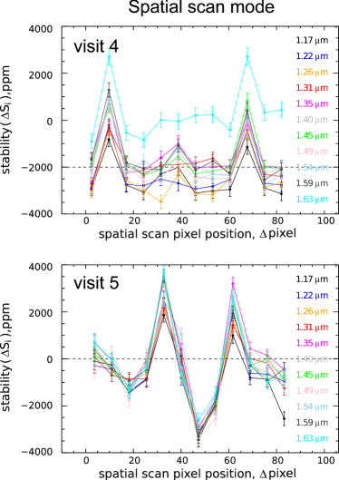
Figure 5: The spatial profile of the $\Delta S_{i}(\lambda)$ values for 11 spectral channels (spatial scan visit 4, see also Figure 3); ideally all values should be zero within the errors and departures from zero shown here represent systematic errors. There is a clear dependence of the measurement property on location with measurement changes (nonrepeatability) of up to $\sim 2000$ ppm. The details of the spatial profiles change from visits to visit; in other words, the pixel-based location of measurement errors does not appear to be constant from visit to visit.

5 Conclusions

We compare the WFC3 stare and spatial scan observing modes in terms of differential spectroscopy measurement performance and conclude that, in terms of stability and repeatability, the stare mode is superior. We show that the spatial scan observations exhibit non-Gaussian behavior and suffer from significant excess measurement noise that is traceable to changes in instrument behavior for different regions of the focal plane. This spatial-temporal variability creates excess noise at the level of $\sim 2\times$ the photon noise that is relatively invariant for changes in spectral resolution. The spatial-temporal variations correspond to a measurement error contribution of up to $\sim$75 ppm per pixel per hour. If other HAWAII-type detectors have similar behavior, multiobject calibration approaches may be limited to $\sim$1000 ppm measurement precision. For JWST, which will use the long wavelength H2RG detectors, careful investigation of the spatial-scan noise and development of calibration methods is likely crucial to achieve the full scientific potential of the observatory for characterizing exoplanet atmospheres.

Only twice, this and one previous time, have large numbers of WFC3 orbits ($>60$) been systematically analyzed for measurement properties at the level of individual sample-up-the-ramp detector reads. In both cases, evidence of systematics appeared that (1) could not be revealed by the analysis of data averaged to the detector integration time, (2) showed some instrument modes were better than others, and (3) found that measurement performance in some instrument modes is variable at the visit-to-visit time scale. The approach of working with a time series of individual detector sample-up-the-ramp reads allows for the detection of systematic changes in eclipse depth or a stability measurement metric that are correlated with detector read. It also provides a natural mechanism to handle saturated observations, which occurs for a surprising number of the WFC3 exoplanet observations.

6 Acknowledgements

The authors thank Mark Colavita and Ingo Waldmann for comments on this manuscript. The research described in this publication was carried out in part at the Jet Propulsion Laboratory, California Institute of Technology, under a contract with the National Aeronautics and Space Administration. Copyright 2013 California Institute of Technology. Government sponsorship acknowledged. All rights reserved.

References

- Berta et al. (2012) Berta et al. 2012, ApJ, 747, 35
- Deming et al. (2013) Deming, D. et al. 2013, ApJ, 774, 95
- Huitson et al. (2013) Huitson et al. 2013, MNRAS, 434, 3252
- Mandell et al. (2013) Mandell, A., Haynes, K., Sinukoff, E., Madhusudhan, N., Burrows, A., Deming, D. 2013 arXive1310.2949
- McCullough & MacKenty (2013) McCullough P. & MacKenty J. 2012, ISR WFC3 2012-08
- Swain et al. (2013) Swain, M.R., et al. 2013, Icarus, 225, 432
- Stevenson et al. (2013) Stevenson, K.B., Bean, J.L., Seifahrt, A., Desert, J-M, Madhusudhan, N., Bergmann, M., Kreidgerg, L., Homeier, D. 2013 arXiv1305.1670
- Tinetti et al. (2013) Tinetti, G., Deroo, P., Swain, M. R., Griffith, C. A., Vasisht, G., Brown, L. R., Burke, C., McCullough, P. 2010, ApJ, 712, 139
- Wakford et al. (2013) Wakeford et al. 2013, MNRAS, 435, 3481