On extended sign-changeable interactions in the dark sector
Abstract
We extend the cosmological couplings proposed in Sun et al. and Wei, where they suggested interactions with change of signs along the cosmological evolution. Our extension liberates the changes of sign of the interaction from the deceleration parameter and from the relation of energy densities of the dark sector and considers the presence of non interactive matter. In three cases we obtain the general solutions and the results obtained in models fitted with Hubble’s function and SNe Ia data, are analyzed regarding the problem of the cosmological coincidence, the problem of the crisis of the cosmological age and the magnitude of the energy density of dark energy at early universe. Also we graphically study the range of variation of, the actual dark matter density parameter, the effective equation of state of the dark energy and the redshift of transition to the accelerated regimen, generated by variations at order in the coupling parameters.
I Introduction
Cosmological and astrophysical data from type Supernovae Ia (SNeIa) data, Cosmic Microwave Background (CMB) radiation anisotropies and Large Scale Structure (LSS), have provided strong evidences for a phase of accelerated expansion of our spatially flat universe Supernova ; SDSS ; Spergel:2003cb ; Dark . The dominant components in our current universe are dubbed dark energy (DE) and dark matter (DM) because of they share a non luminous nature. They behave very differently, while DE has negative pressure and is responsible for the aforementioned acceleration, DM is gravitationally attractive and allows the accumulation of matter that leads to the formation of large scale structures. Only hypotheses on their nature exist, most of them assuming that DM and DE are physically unrelated and the similarity in their energy densities (the so called problem of Cosmological Coincidence) is a purely accidental fact Wetterich:1987fmyRatra:1987rm ; Peebles:2002gy ; Kolb:2005da . But interactions between DM and DE might alleviate the problem, keeping close values for their densities up to large redshifts as has been shown in a lot of work Ellis_Wetterich_Amendola_Gasperini ,interacc , Chen:2011cy . The interactions between DE and DM appear to be favored in several works, for instance, by Bertolami et al. Bertolamivarios through studies on the Abell Cluster A586, and Abdalla et al. where they found the signature of interaction between DE and DM by using optical, X-ray and weak lensing data from 33 relaxed galaxy clusters Abdalla:2007rd . Their conclusions are that this coupling is small but indicates that DE might be decaying into DM. Based on the detail analysis in perturbation equations of DE and DM when they are in interaction, He et al. find that the large scale CMB, especially the late Integrated Sachs Wolfe effect, is a useful tool to measure the coupling between dark sectors and arrive at the same conclusion He:2009pd . Although the observational constraints indicate the possibility that the decay can be in both directions, Guo:2007zk ; Quartin:2008px , the decay of DE into DM seems to be strongly favored from a thermodynamical perspective, provided that the chemical potential of both components vanish or even without considering the chemical potential,Pavon:2007gt . Other authors argue that If the chemical potential of at least one of the fluids is not zero, the decay can occur from the DM to DE, with no violation of the second law Pereira:2008at ; Lima:2008uk ; Pereira:2008af ; Pereira:2008nd . Also, in Olivares:2008bx a restriction on the interaction parameter strength are obtained, discarding interacting models with constant coupling strength greater than 0.1 at confidence level. This constraint has been obtained for the particular case of an interaction in the dark sector, which is proportional to the total energy density when other components are not considered. Without a firm theoretical basis to raise the type of coupling, interactions are proposed and analyzed for compatibility with a number of basic premises arising from the huge amount of observational data. The cosmological coincidence problem (CC), the bounds on the dark energy density parameter in the early universe (EDE), the magnitude of the EoS of dark energy in the present and in the recent past, the possibility or necessity of nonzero pressure of dark matter, the problem of having milestones older than the age of the universe, the existence and variability of the transition redshift, are all matters to meet with the interaction under study. In addition, recently one has found that the interaction can change its sign, in contemporary times with that of the transition to the accelerated regime and not too distant to it, cosmologically speaking, but not necessarily coincidental with it Cai:2009ht . In light of these considerations, among the various possible interactive proposals, Cai’s work indicates that should be selected those which can change its sign along cosmological evolution. There are a few papers Changeable , where the proposals are explicit but analytical solutions are obtained only in some cases. In this paper we propose an extension of these works, considering interactions where the deceleration parameter and the interaction do not change their signs together but with a short time delay and also, a baryonic component that is not coupled to dark sector is added. The selected sign-changeable interactions used here affect only the dark sector and in all proposed cases, our work generates exact solutions. We analyze their behaviors through models whose parameters are adjusted minimizing a function Press with the Hubble data Stern:2009ep ; Simon:2004tf ; Moresco:2012by ; Farooq:2013hq ; Liao:2012bg , and SNIa observations Riess:2009pu . The H(z) test was probably first used to constraint cosmological parameters in Samushia:2006fx and then in a large number of papers Wei:2006ut ; Lazkoz:2007zk ; Lin:2008wr ; Cao:2011cg ; Figueroa:2008py ; Seikel:2012cs ; Santos:2011cj ; delCampo:2010zz ; Aviles:2012ir . In the next section we present the general framework which describes the dark sector with an exchange of energy and the evolution of the non interacting fluid. After that, in section III, we analyze explicit interactions with worked examples based on models with adjusted parameters. In section IV we compare the results obtained and in the last section, we summarize our main outcomes and conclude.
II The models
We consider cosmological models with two interacting dark fluids plus a non interacting baryonic component in flat Friedmann Robertson Walker metric (FRW). The dark sector contains a dark matter fluid with energy density in interaction with a dark energy fluid with energy density . The scenario is completed with a not interactive matter component with energy density that at first, can be dust or radiation. We have assumed that the equations of state (EoS) are for constant barotropic indexes , . Also, we have defined an auxiliary ”dark” barotropic index and the overall effective barotropic index . The Friedmann equation and the conservation equation are given by
| (1a) | |||
| (1b) |
| (2a) | |||
| (2b) | |||
| (2c) |
Above and henceforth ′ means derivative with respect to the variable and , and are the factor of scale for the FRW metric, the actual factor of scale and the Hubble parameter respectively. Using (1b), (2b) and (2c) the partial energy densities , and can be written as
| (3a) | |||
| (3b) | |||
| (3c) |
The interaction , that is only applied to the dark sector, is defined through the splitting of the equation of conservation (2b) as
| (4a) | |||
| (4b) |
Once the interaction is fixed, the dynamic evolution of the auxiliar dark EoS is obtained solving the integro-differential equation
| (5) |
Sometimes, the general solution of (5), , can be integrated to obtain the expression of the energy density of the dark sector . In such cases, we have all the necessary information to know the partial dark densities through the equations (3), the dark ratio , the effective EoS for the dark sector , the deceleration parameter and the effective partial state equations and . With that knowledge, we obtain the explicit expression of , and as well, the benefits or defects of each interaction can be calibrated. Among other things, we can analyze if the density parameter of dark energy at early times (EDE) respects the constraints arising from the baryogenesis; if the redshift of sign change is consistent with the results of Cai et al., and if the magnitude of the ratio r in the final stage of the universe alleviates the coincidence problem and to what extent it does. A variety of interactions, which can change its sign, has been proposed Changeable . The Wei’s work matches with the transition redshift to an accelerated universe , while Sun et al. linking with a redshift for which the dark ratio r equals the inverse of the coupling constant (really there, only the case is considered). These studies limit themselves to the dark sector. In the following sections, we extend these studies proposing models with interactions in the dark sector, that show no explicit connection between both redshifts, and plus a fluid satisfying its own conservation equation.
III SIGN-CHANGEABLE INTERACTIONs
Literature does not provide a natural guidance from fundamental physics on the cosmological interaction and so we can only discuss it to a phenomenological level. The most familiar cosmological interactions used are proportional to the energy densities , and , and these magnitudes always can be written in terms of the energy density and of its derivative . So, it seems natural that interactive term corresponds to linear combinations of this type or more generally, that be a non lineal function . In general the models with linear combinations do not allow realizing a change in the direction of transfer of energy between DE and DM and we do not know a solid theory which provides a Lagrangian to derive the appropriate interaction term. Therefore, we propose phenomenological multiplicative terms including the deceleration parameter plus an statistically adjustable degree of freedom that allows differentiate the transition deceleration - acceleration of the universe of the directional transition on the transfer of energy. That is, we propose non linear functions .
III.1
The sign-changeable interaction
| (6) |
is a natural extension of that proposed by Wei (and solved for ), which is reobtained when and are null. It can be written in terms of the auxiliary ”dark” barotropic index , using (2b) and (3b) as
| (7) |
For this option, the equation (5) results into two different first order differential equations for depending on, whether or not is zero:
III.1.1
In the case , the interaction (7) leads to the first order differential equation for
| (8) |
whose general solution is
| (9) |
with and . From (2b) and (9) we obtain the general solution for
| (10) |
where and are constants of integration.
The solutions (9) and (10) allow to obtain, through the expressions (1a) and (3), the functional forms of the total energy density , the partial energy densities and , and the dark ratio ,
| (11) |
| (12) |
| (13) |
and
| (14) |
where , , and is the actual total energy density.
The explicit expressions for the interaction , the deceleration parameter , the density parameter for the dark energy , and the effective equations of state , and , are
| (15) | ||||
| (16) | ||||
| (17) |
| (18) | ||||
| (19) |
| (20) | ||||
where , .
Here and in the following cases we provide a better approach to the interaction, studying its behavior with models whose parameters have been adjusted using the Hubble data as in Stern:2009ep ; Simon:2004tf ; Press . The statistical analysis is based on the minimization of a function with the Hubble data which is constructed as
| (21) |
where stands for cosmological parameters involved in the specific interaction , is the observational H(z) data at the redshift , is the corresponding uncertainty, and the summation is over the 29 observational H(z) data Liao:2012bg . In this case, where and is taken from (11), we find , corresponding to , for the best fit values: , , , , , , and .
Then, the best adjusted model for , exemplifies a universe with interaction between cold dark matter (CDM) and cosmological constant in presence of non-interacting dust. See Table 1.
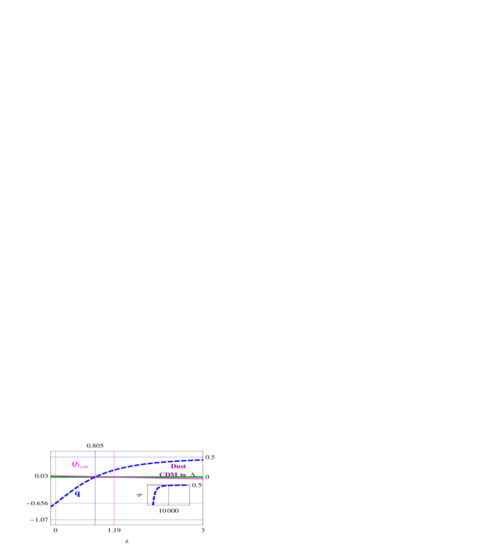
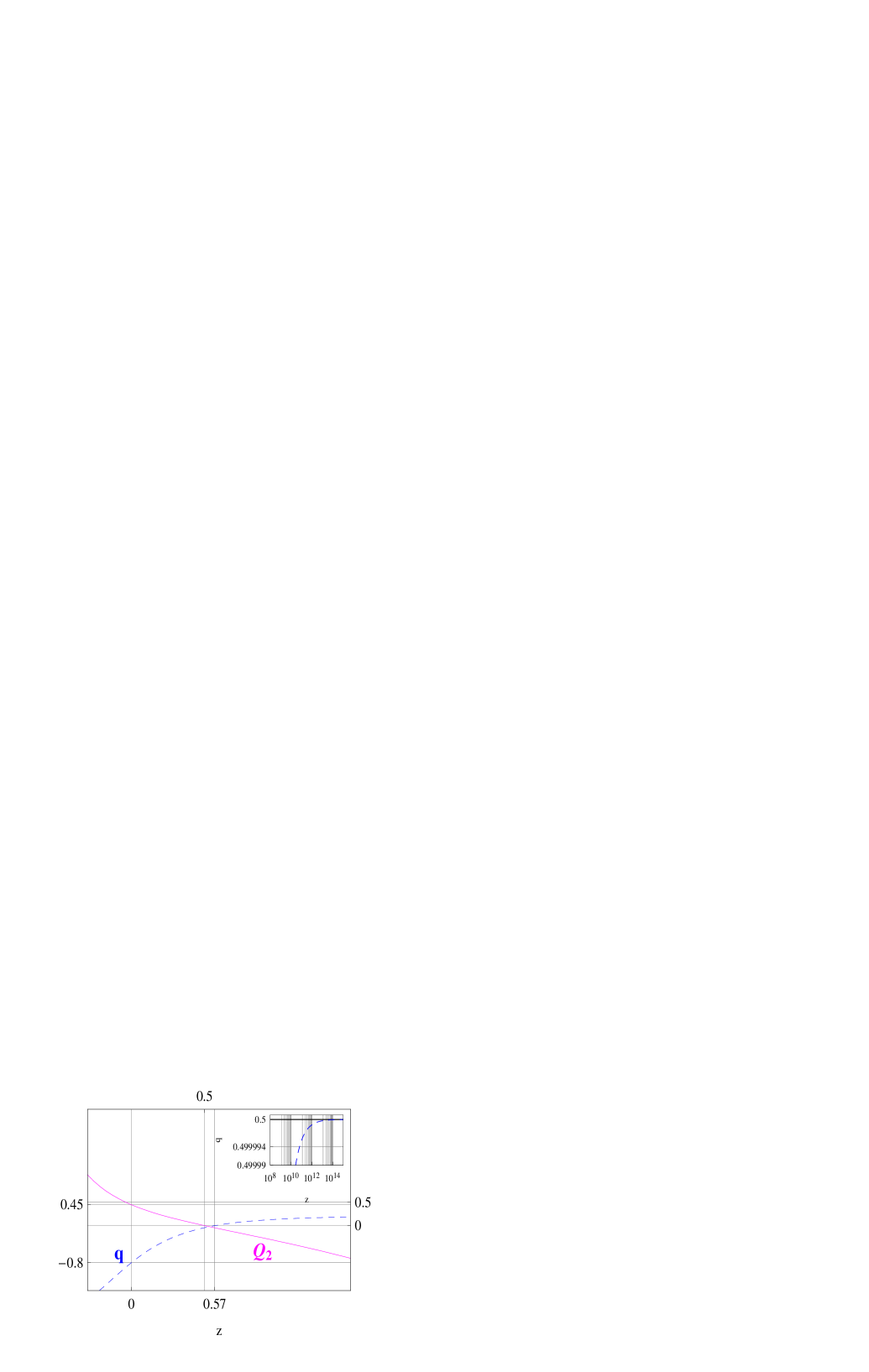
In Fig.1 we show how the interaction progresses from negative values in the past, up to the actual value changing its sign at . Also, we see that the deceleration parameter has asymptotic values at early times and in the far future, transits from a decelerated universe to an accelerating one at while its actual value is . All these values are very much like those of the CDM model, perhaps because most non interactive dust, is dark, as it can be seen in Fig.2 and in Table 2. However, the interaction effect is observed as a delay in transition redshift (about ) respect to a CDM with the same material density parameter . The strength of the interaction in this model is consistent with the result obtained in Olivares:2008bx which sets an upper bound ( at CL) through the discrepancy between the fraction of DE necessary to explain the amplitude of the ISW effect larger than the allowed by the WMAP data.
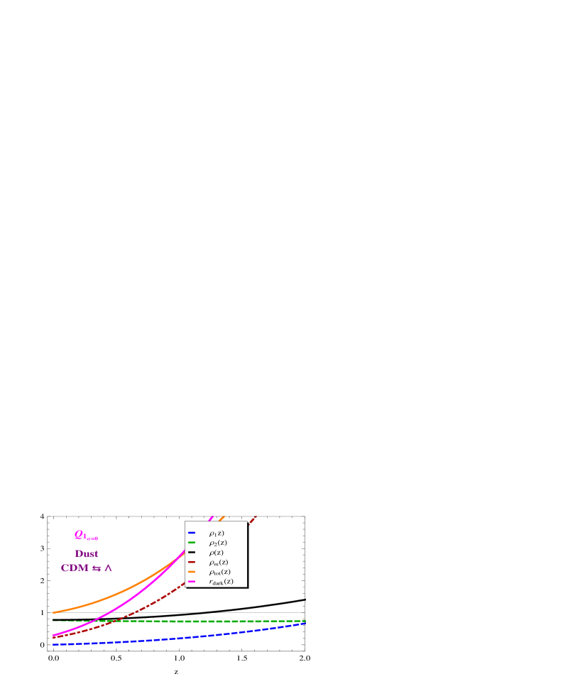
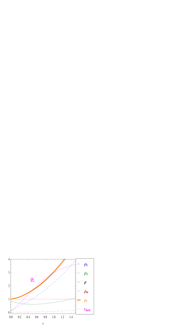
The Fig.2 shows the evolution of all energy densities involved in the model and the dark ratio between DM (interactive and non interactive) and DE fluids, that takes the value 1 around .
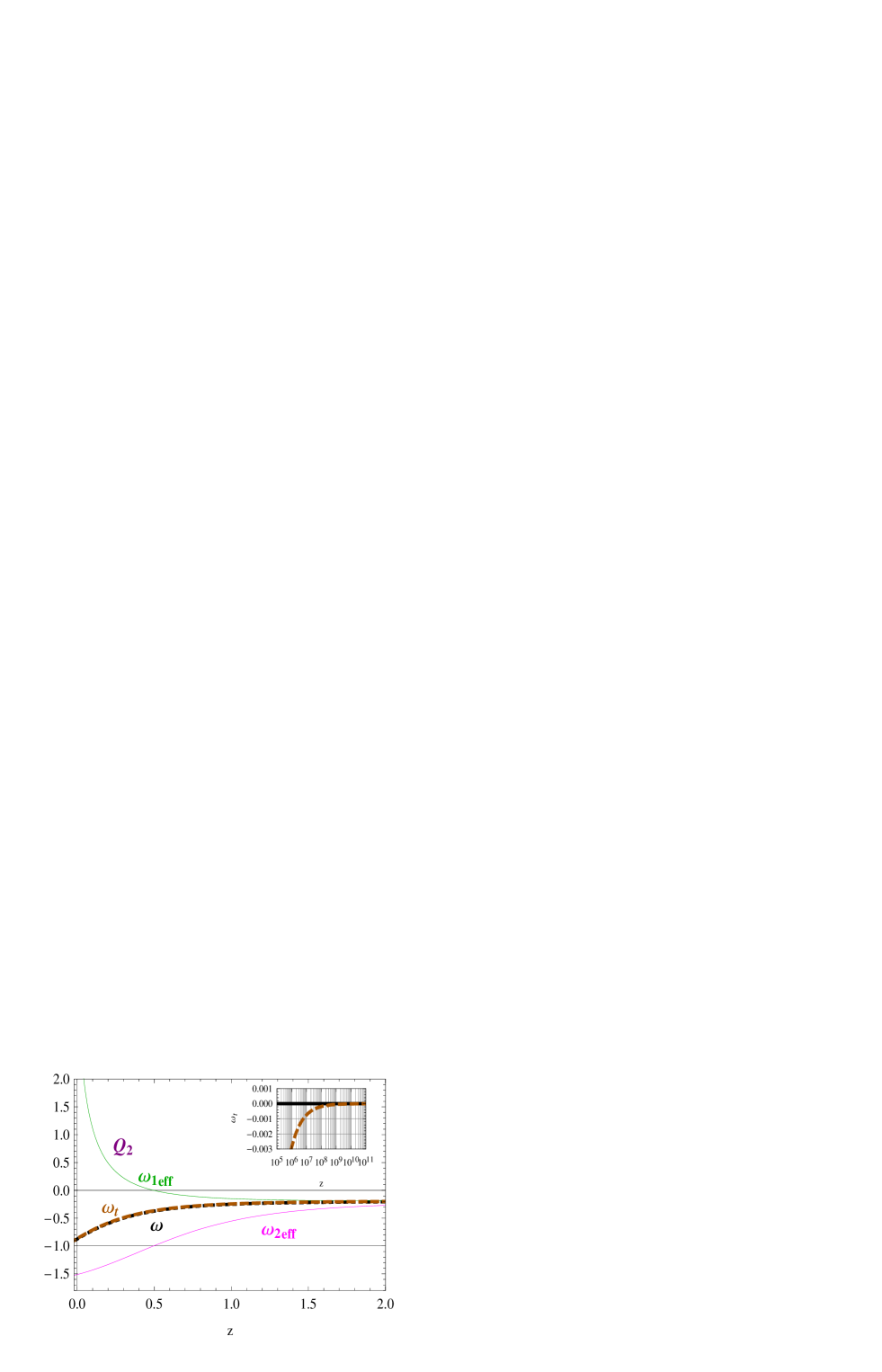
The evolutions of all effective equations of state are shown in Fig.3, where we can see that at early times, and , both tend to zero, showing the absolute dominance of dust fluid. The inset shows that the dark energy fluid has an asymptotic value at early times and crosses the phantom divide line (PDL) just before the present time where has the value . We are interested in knowing how the magnitudes of the energy density parameter , the effective EoS of dark energy and the redshift of the transition to the accelerated regimen are affected because of the variations in the coupling parameters and . For this task we take the CL intervals and , (see Table 2).
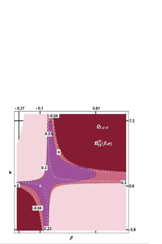
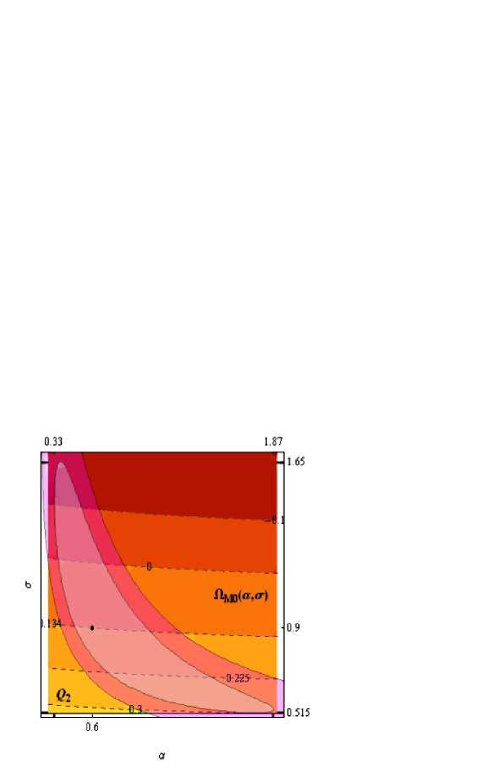
A graphical way of knowing the range of variation of the current total matter content, caused by changes in and , is throughout the overlapping of the confidence region for these coupling parameters, on the contours graph of the present matter content in the vs. parameter space for the best fit model. The restriction on the possible present values of plus in the case can be seen in Fig.4 where the confidence region (lila region) restricts so that its present values belong to the interval . Also in this two-dimensional graph, we can see the CL, , and the best fit value for the matter parameter (white dot).
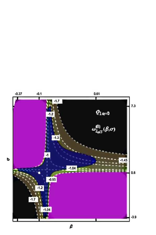
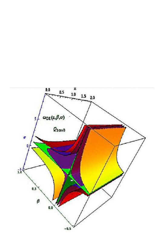
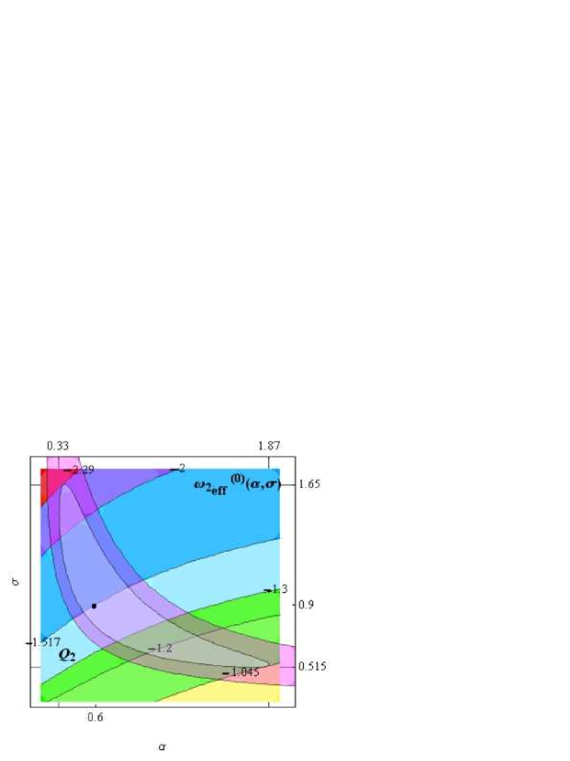
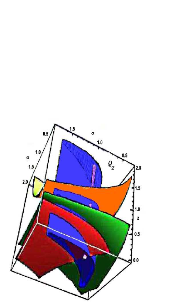
The characteristic parameter of dark energy, its effective equation of state , deserves some further study. Its variation with the parameters that identify the interaction, and , can be seen in Fig.5, where the region corresponding to the CL in the parameter space vs. (blue area), is superimposed on the contour plot of the current . The resulting information is that the actual effective dark energy EoS is . For clarity, Fig.4 and Fig.5 are presented complete although only negative values of are allowed by the positivity of . Moreover, from the three dimensional Fig.6, we can see the evolution of between and at CL in the vs. region. The plot shows that best fit white line crosses the phantom divide plane (green plane) just before the current time and that, in that redshift interval, the EoS of the dark energy fluid is always between the yellow plane and the red plane at least for values of , belonging to their CL.
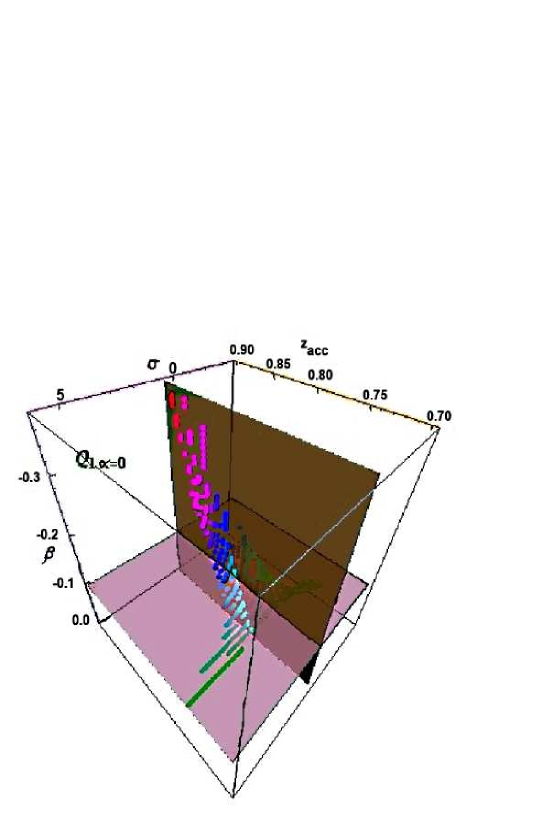
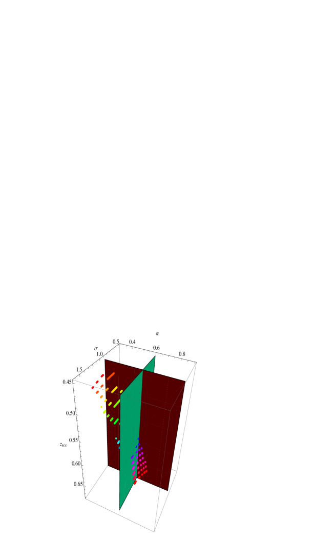
The crossing of the red plane occurs only for , but the positive values are excluded for because they lead to . This result is in good agreement with the constraints on the evolution of the dark energy equation of state derived from a dataset for several dark energy models as Hu-Sawicki, tracking SUGRA and tracking power-law Said:2013jxa ; Fang:2008sn ; Ade:2013zuv . The variation of the parameters and also affects the redshift of the transition to accelerating universe. Fig.7 shows that with variations on the coupling parameters at CL, the transition value belongs to the interval being an increasing function of and decreasing one of , much more sensitive to changes in than to changes in as we can observe on brown constant plane and on green constant plane . This best fit value for the transition redshift is significantly higher than that obtained in Cunha:2008ja at CL analyzing distinct databases and in a model-independent way. However, it is typical for models with interactions in the dark sector Chimento:2007yt ; Chimento:2011dw ; Chimento:2013se ; Chimento:2007da ; Forte:2012ww ; Farooq:2013hq .
We can estimate the age of our universe using the time-redshift relation
| (22) |
and also qualify the interaction, at least with respect to the coincidence problem, through the fraction of T for which the ratio between dark sector densities remains around the unity. That is, if for the interaction , it turns out that from until today is , then the magnitude
| (23) |
gives us a good idea of the benefits of the interaction under study respect to that issue. In the particular case with its best fit model, the coincidence seems to be satisfied for (see Fig.2). Therefore, replacing (11) in (22) it turns out that the best fit model has a good score with Gyr.
III.1.2
When the term in is included in the interaction (6), the evolution equation for the auxiliary dark barotropic index is
| (24) | ||||
where
| (25) |
Looking at the solution (26) for , it is apparent that an explicit expression for , and subsequently for can be obtained only in special situations, where A or B are canceled, or are inverses one of each other. All these special cases correspond to choosing a particular value for the coupling constant of the interaction, for respectively.
-
•
In this case is fixed at the value and therefore the explicit expressions for and are(27) (28) where and are constants of integration. From equations (3), (27) and (28) we obtain the explicit expression of all interesting variables of the case, the total energy density , the partial energy densities and , and the dark ratio ,
(29) (30) (31) and
(32) where , , and is the actual total energy density.
Also, we obtain the explicit expressions for the interaction , the corresponding deceleration parameter , the density parameter for the dark energy , and the effective EoS , and ,
(33) (34) (35) (36) (37) (38) where and with .
Here, the best-fit model through the minimization of the function (LABEL:020), where the theoretical Hubble function is taken from the equation (LABEL:016), corresponds to a minimun or . The set of parameters is with the best-fit values , , , , , , and . With these values we can say that the model belongs to a scenario of warm dark matter (WDM) fluid interacting with a cosmological constant in presence of non-interactive dust. Conveniently, the best fit value for is negative, which keeps positive the energy density of DE at any time in the past. The nickname WDM is used here in the following sense. The perfect gas equation of state may be written as with the particular gas constant R and the temperature T. is a characteristic thermal speed of the molecules and if is the speed of light, the EoS is a measure of the energy of the matter directly related to its typical temperature Carter:1987qr . In this sense, we call lukewarm or generically, warm matter, (baryonic or dark), to that has a lightly positive EoS (), reserving the expression “cold matter” for the case of EoS strictly zero. The issue of the dark matter component with a small but non zero pressure was studied in Harko-Lobo:2012 ; Bharadwaj-Kar:2003 ; Su-Chen:2009 ; Saxton-Ferreras:2010 ; Lim:2010yk in the context of modeling galaxy halos. Also in Moore:1999gc ; Bode:2000gq ; AvilaReese:2000hg ; Dalcanton:2000hn ; Boyanovsky:2010pw ; Destri:2012yn , WDM particles were invoked as possible solutions to both, the over prediction of satellite galaxies, by almost an order of magnitude larger than the number of satellites that have been observed in Milky-Way sized galaxies and as a mechanism to smooth out the cusped density profiles predicted by CDM simulations.
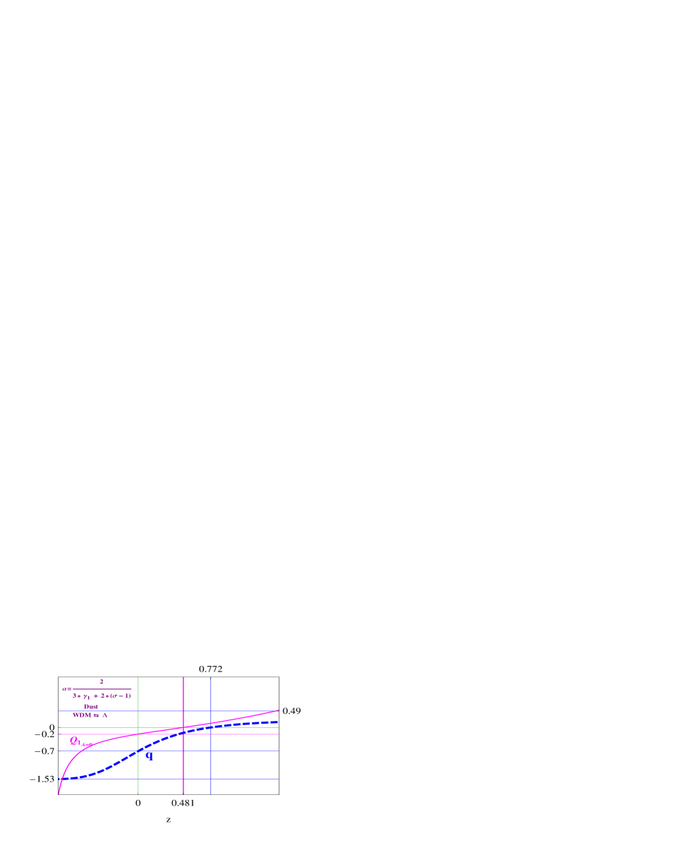
Figure 8: Evolutions of the interaction (33) and its corresponding deceleration parameter (34), in the case for the best fit model (), with , , , , , , , and . The transition to the accelerated regime is verified at and the actual deceleration parameter value is . The interaction changes its sign at , from which begins to transfer energy from DE to DM. The gradient of this interaction between the present epoch and the time when it reverses its sign, is an order of magnitude greater than in the case of . 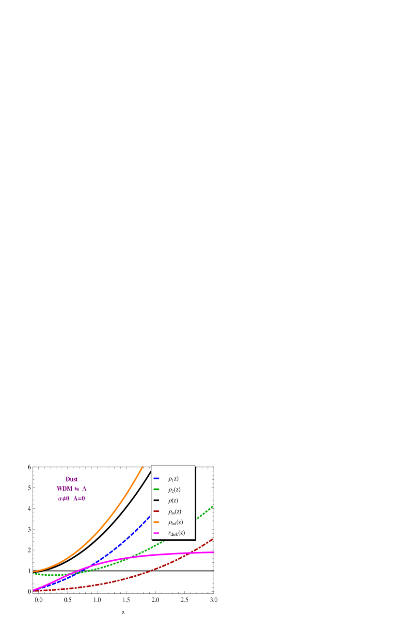
Figure 9: Evolution of all energy densities involved in the best fit model with interaction in units of . Interestingly, most of the total energy density is supplied by the dark sector throughout the evolution. The ratio of dark energy densities becomes of order 1 around , much earlier than in the previous case and this is extended up well back in time. In Fig.:8, the interaction and the corresponding deceleration parameter are depicted as functions of the redshift. In this model there is strong energy transfer from the particles of warm dark matter to DE at early times and the situation is equally serious, but in the opposite direction, in the distant future. Instead, in recent history the transfer is relatively smooth, only one order of magnitude greater than for , and WDM particles decay into DE until when its effects are reversed causing the creation of WDM particles. For , tends asymptotically to a value very similar to the CDM at early times. The same is true for the current time when but in the far future this model is a fifty percent more accelerated. The Fig.:9 shows the evolution of all energy densities , , , and for the best fit model and also the ratio for this particular interaction. There it can be seen that the full coincidence between the magnitudes of the dark densities occurs around , before than in the previous case , and remains in the same order until well back in time. A notable feature is that the total energy is mainly composed of energy of the interacting dark sector, and that it varies much more violently than in the previous case. The evolutions of all effective EoS, whose early - time asymptotic values are , and , are shown in Fig.:10. The effective EoS of DE crosses the PDL around but, notably, coming from more negative values. This crossing is treated in a lot of works QuintomsFeng:2004ad and particularly, it is considered in HutererCooray where a passage from the value at to the value at is obtained through the Gold set of SNe Ia. The actual EoS are , and .
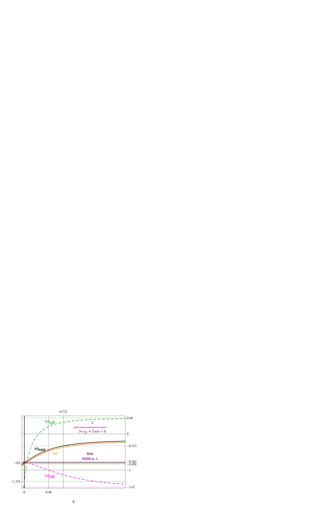
Figure 10: Evolution of all EoS in the best fit model with the interaction . At early time the global effective fluid behaves as dust while the asymptotic effective values of the dark EoS are and . The crossing of PDL is carried out by the effective DE around , while the actual values of the effective EoS are , and . The current matter content (WDM plus baryonic cold matter) is graphically constrained in Fig.:11 where confidence regions at level and for coupling coefficients and are plotted on the contours of . The permissible values for total matter content correspond to the range at CL in vs. space and at CL while the best fit is . These ranges are in good agreement with the results found in the literature Kessler:2009ys ; Sullivan:2011kv ; Suzuki:2011hu .
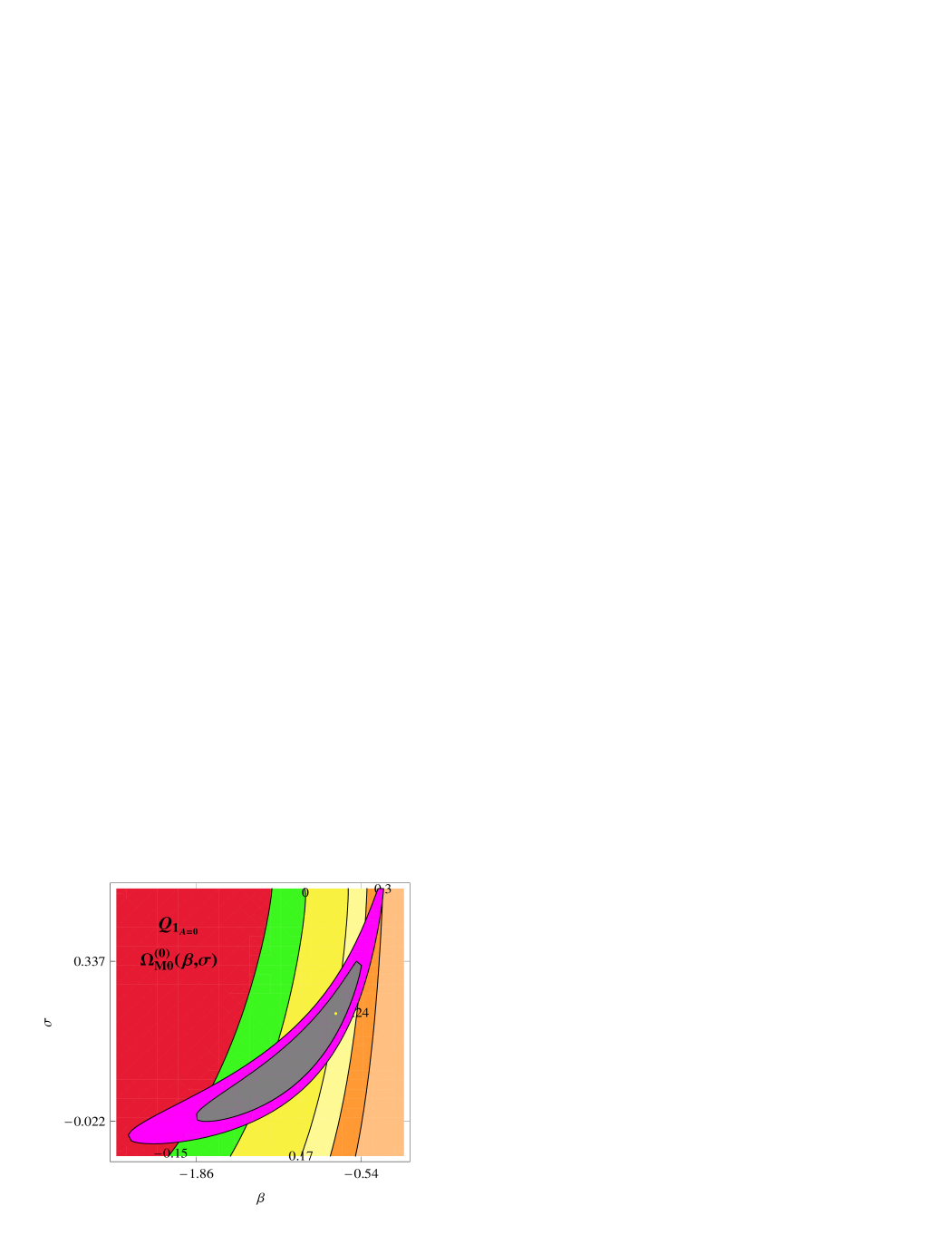
Figure 11: and confidence regions for the parameter space vs. overlapping the sum of the two actual density parameters of matter (WDM and baryonic cold matter) in the case with . From the contours of the density parameter we can infer that non-negative values, that is, the permissible values for total matter content correspond to the range at CL and at CL while the best fit is . With the same graphical technique, the effective EoS of DE at the present time is constrained giving the range at CL in vs. space, as seen in Fig.:12. From these contours one can infer that the value of is not favored even at CL in vs. space.
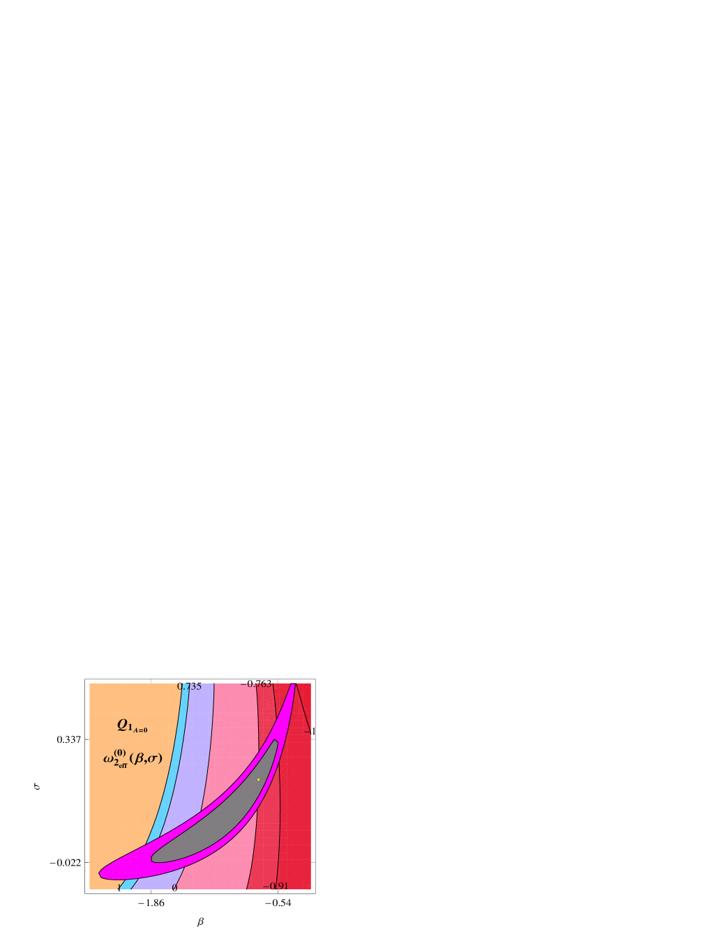
Figure 12: and confidence regions for the parameter space vs. overlapping the actual effective EoS of dark energy in the case . From the contours of one can infer that for variations of and at CL, the values of the actual effective dark energy EoS belong to the range . The value is not favored even at CL, while the best fit is . With the three-dimensional graph of Fig.:13, obtained by intersecting the CL ellipses in each instant between and (yellow surface), on level surfaces , we can extend the above analysis to study the evolution of these constraints in the redshift range . The contours considered are (red surface), (green surface) and (light blue surface). The pink line, which represents the evolution of for the best fit model, does not cross the light blue surface when . Instead at CL in vs. space, yes it does and at CL the crossing of the PDL is carried out between and . Again, this is in agreement with literature Nesseris:2006er .
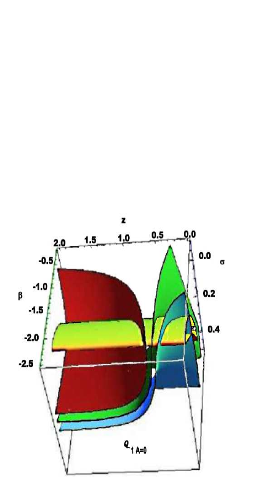
Figure 13: Evolution at CL of the effective EoS of dark energy in the case . The figure is obtained by superposition of the CL surface (yellow surface) for the space vs. vs. and the contours (red surface), (green surface) and (light blue surface). It can be seen that the best fit white line does not cross the light blue surface when (but at CL yes it does), and that at CL the crossing of the PDL is carried out between and . 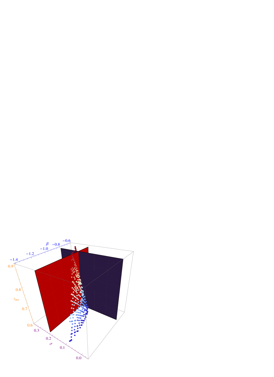
Figure 14: Variation of the transition redshift in the best fit model with the interaction , at CL on parameter space vs. . The constant black plane corresponds to and the constant red plane to while the dots hold the conditions , and . The relation is an increasing function of and a decreasing one of . The three-dimensional Fig.:14 represents the variation of the transition redshift in the case with interaction , due to variations at CL on parameters and . The constant black plane corresponds to and the constant red plane to while the dots hold the conditions , and . In this context, the relation is an increasing function of and a decreasing one of . The best fit model for the case has . Therefore, replacing (29) in (22) it turns out that this interaction has , better than the previous coupling and its cosmological age is Gyr.
-
•
or
When any of the options is satisfied, the condition arises from the equation (25) and then, equations (4b) and (6) say us that this condition implies that is a constant, . That is, . The interactions that satisfy the requirement have , and then they are not of our interest because they do not solve the problem of the coincidence.
III.2
This interaction is the natural extension of the Sun Yue proposal, which is recovered when and , and leads to the first order equation
| (39) |
The general solution of (39)
| (40) |
with the constants
| (41) |
allows to obtain the general solution of for the energy density of the dark sector ,
| (42) |
where and are constants of integration.
With the expressions (3), (40), (41) and (42) we can obtain all the explicit functions of the redshift describing the total energy density , the dark single energy densities and , the ratio , the interaction, the deceleration parameter , all the effective EoS , and and the density parameter of the dark energy :
| (43) |
| (44) |
| (45) |
| (46) |
| (47) |
| (48) |
| (49) |
| (50) |
| (51) |
| (52) |
with , , and .
In this case, where and is taken from (43), we find , corresponding to , for the best fit values: , , , , , , and . That is, the best adjusted model for , supports an interaction between CDM and cosmological constant in presence of non interactive dust. In Fig.:15, the interaction and the corresponding deceleration parameter are drawn as functions of the redshift. In this model there is strong energy transfer from DE to the particles of CDM at early times and equally strong is the energy transfer from the CDM decaying into DE in the distant future. Instead in recent history, the transference is relatively smooth and CDM particles creation ceases from when its effects are reversed. For , tends asymptotically to a value mimicking CDM at early times and the same is true for the current time when . This value coincides with the correspondent to the model CDM, calculated with the parameter of density of both, interactive plus not interactive dust and the transition redshift is consistent with the values consigned in literature Lima:2012bx , Cunha:2008mt ,Liu:2012me , (See Table 2). Fig.:16. shows the evolution of all energy densities , , , and for the best fit model and also of the ratio for this interaction. It can be seen that the relation between the magnitudes of dark densities is around , (later than all the previous cases) and that the total energy is mainly composed of energy of the interacting dark sector. Notably, the dark energy density decreases monotonously until when it begins to recover, growing up to the current time reflecting the change of sign of the interaction. The evolutions of all effective EoS, whose early - time asymptotic values are and , are shown in Fig.:17. The effective EoS of DE crosses the PDL around , redshift almost coincident with the redshift of the transition to the accelerated regime, . The variations of the actual value of the total matter content and of the effective EoS of DE due to variations at CL of the coupling parameters in the case are drawn in Fig.:18 and Fig.:19. In the first of these two graphs, the error ellipse for vs. parameters space, superimposed onto contours of sum of the density parameters , shows that . In the second graph, the same error ellipse indicates that the actual . The Fig.:20 is a sample of evolution of the effective equation of state of DE where it can be seen that the best fit model for (solid pink line), crosses (red plane) just before the actual time and at CL in vs. parameters space, it crosses the phantom divide line (green plane) between and . The yellow plane corresponds to contour . Finally, the effect of varying the coupling parameters at CL onto the transition redshift to the accelerated phase is shown in Fig.:21, where it can be seen that is a strongly increasing function of and a growing one respect to but with little sensitivity. This behavior is reflected on the constant planes (cyan) and (brown). Its values belong to the interval when and .
IV Comparisons
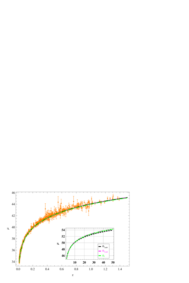
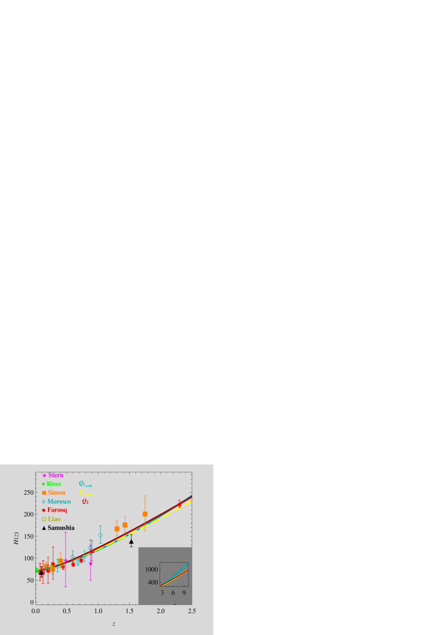
The curves of distance modulus for the models with the better adjusted parameters are compared in Fig.:22 with the SNIa Union2.1 database Suzuki:2011hu for these three interactions. Their behaviors are identical and fit very well to the experimental data. The difference among the theoretical curves are only seen at higher redshifts as shown in the inset for the interval between and . This means that the supernova data are not the appropriate tool to choose among these models because Union2.1 upper bound corresponds to a redshift and the curves are separated later. Better discrimination is obtained on Fig.:23 where the curves corresponding to the theoretical Hubble functions of the three models are compared between themselves and with respect to the Hubble data function Stern:2009ep ; Riess:2009pu ; Simon:2004tf ; Moresco:2012by ; Farooq:2013hq ; Liao:2012bg . There it can be seen that they are very similar in the range defined by the data but later, they differ for higher redshifts forming two distinct groups. On one hand, the case with and on the other, the cases with and , are two different sets as it is shown in the inset for the interval between and . These two forms of comparison do not turn out to be satisfactory to incline our preferences in favor of anyone of the studied interactions.
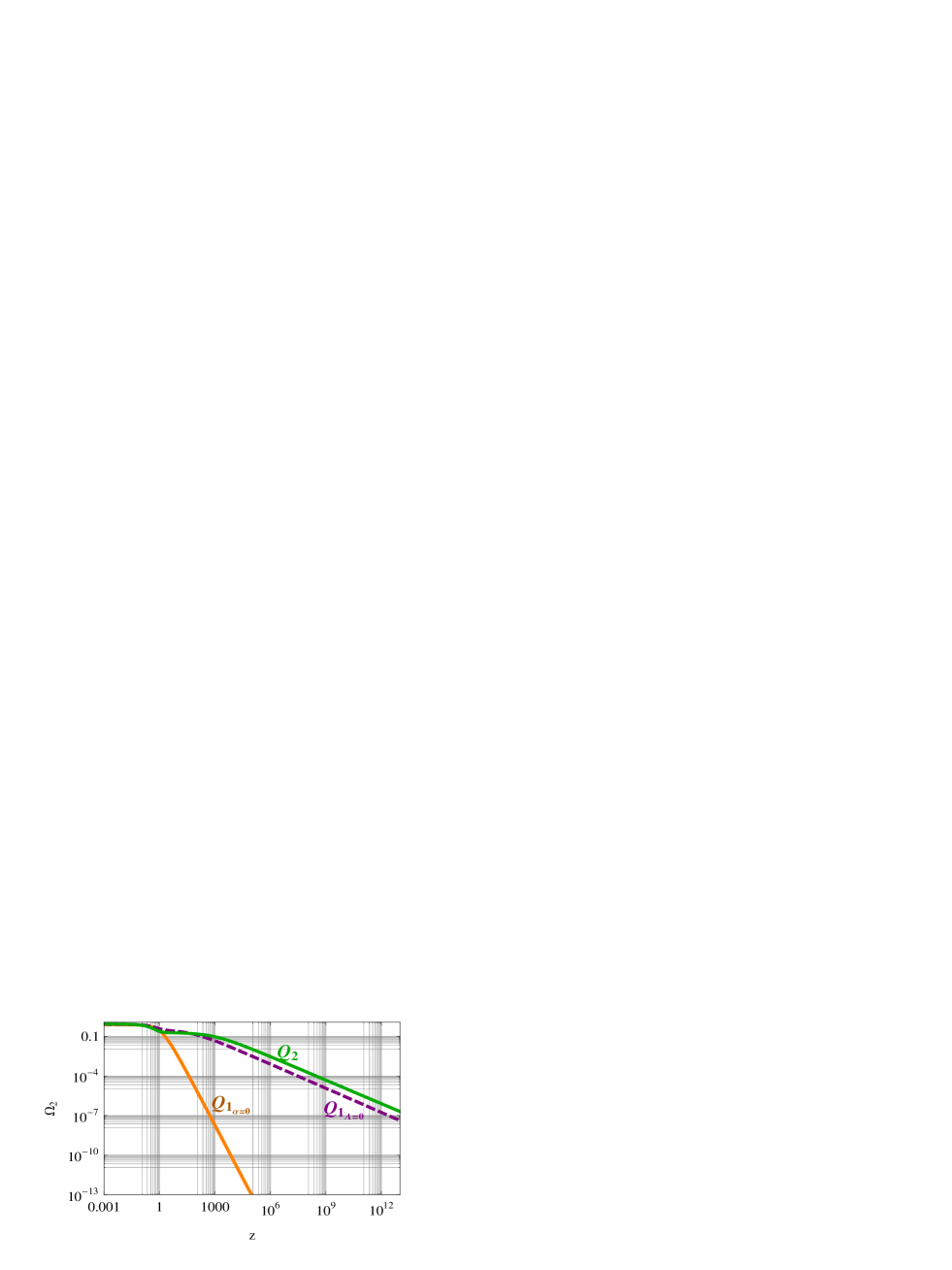
To further explore the suitability of each interaction, we analyze the behavior of dark energy at early times (EDE). Many authors have claimed the existence of a non-negligible dark energy at early times. That is, the dark energy could not fade away to the fraction of the energy density at CMB recombination that is predicted by the cosmological constant. For example, Wetterich proposes the modeling of the vacuum energy by a phenomenological parameterization of a quintessence and draws as conclusion that EDE should necessarily exist, under certain circumstances (parameter , see Wetterich:2004pv ). Moreover, some descriptions of this energy, coming from the field of particle physics, involve scalar fields whose densities correspond to a constant fraction of the energy density of the dominant component Ferreira:1997hj . In addition, Big bang nucleosynthesis (BBN) () can help to determine whether or not there is EDE, constraining the allowable amount of it that does not interfere with the process of nucleosynthesis. The presence of vacuum energy can be seen also, via the expansion speed up provided by this additional energy density. The vacuum energy acts essentially as an extra neutrino species and the bound on the number of species determines a maximum value of the vacuum energy during the baryogenesis era Cyburt:2004yc . Fixing the effective number of relativistic neutrinos to the standard value , Calabrese et al.Calabrese:2011hg , improve the bound yielding in case of a relativistic EDE and for a quintessence EDE, at BBN epoch. Also, Sievers et al. Sievers:2013ica say that the small-scale damping seen in the Atacama Cosmology Telescope (ACT) data can be interpreted as arising from an amount, non-negligible, of dark energy at decoupling and their analysis of the ACT data in combination with WMAP7 data and the ACT detection measurement, leads to the upper bound (WMAP7 + ACT + ACTDfl, at CL), with the bound on the equation of state . The same model used by Sievers, was previously constrained from Reichardt et al. Reichardt:2011fv who reports an upper limit of at CL from CMB only data, combining WMAP and SPT. The first cosmological results of the Planck Collaboration Ade:2013zuv refer to the two main effects of EDE: the reduction of structure growth in the period after last scattering and the change of position and height of the peaks in the CMB spectrum. Note that the possibility of a dark energy late, after the last scattering surface, is dependent on exactly what supplementary data are used in conjunction with the CMB data. Using the direct measurement of , or the SNLS SNe sample, together with Planck shows preferences for dynamical dark energy at about CL reflecting the tensions between these data sets and Planck in the CDM model. In contrast, the BAO measurements together with Planck give tight constraints which are consistent with a cosmological constant. Interestingly, the presence or absence of dark energy at the epoch of last scattering () is the dominant effect on the CMB anisotropies and hence the constraints are insensitive to the addition of low redshift supplementary data such as BAO. The most precise bounds on EDE arise from the analysis of CMB anisotropies Doran:2001rw ; Caldwell:2003vp ; Calabrese:2010uf ; Reichardt:2011fv ; Sievers:2013ica ; Hou:2012xq ; Pettorino:2013ia . Using PlanckWPhighL, (WP stands for a WMAP polarization low multipole likelihood at and highL is the high-resolution CMB data), at CL and for PlanckWP only Bennett:2012zja . These bounds improve the recent ones of Hou:2012xq , who give at CL, and Sievers:2013ica , who find at CL. Calabrese et al. Calabrese:2011nf discuss present and future cosmological constraints on variations of the fine structure constant induced by an EDE component having linear coupling to electromagnetism. They found no variation of the fine structure constant at recombination respect to the present-day value, constraining EDE to at CL. Hollenstein et al. Hollenstein:2009ph constraint EDE from CMB lensing and weak lensing tomography finding a best fit with different errors according to the different experiments and the combinations of Euclid with Planck and CMBPol. In summary, we have a variety of restrictions on the EDE, resulting from its possible action on cosmological structure formation, variation of the fine structure constant, growth of fluctuations in dark matter and primordial nucleosynthesis, but they all refer to models without interaction in the dark sector and there are also considerations about the temporary location (or redshift) at which they must be applied Pettorino:2013ia ; Cahill:2013kda . The Fig.:24 shows the evolution of the curves corresponding to density parameter of dark energy for the three models considered, for which clearly, there are two types of behavior. For the case with interaction (solid orange curve) the slope is very steep and able to accommodate any restrictions, but it is even more negligible than the cosmological constant. In the other two cases, with interactions (dashed purple curve) and (solid green curve), the density parameters decrease more slowly and may be consistent with some bounds obtained from non interacting models. It must be highlighted the fact that the behaviors drawn in Fig.:24 correspond to models with interactions described in the dark sector plus the inclusion of a non-interactive material component, so that before considering whether or not they satisfy the aforementioned constraints, they should be considered as examples of the possible values of EDE in the class of interactive scenarios.
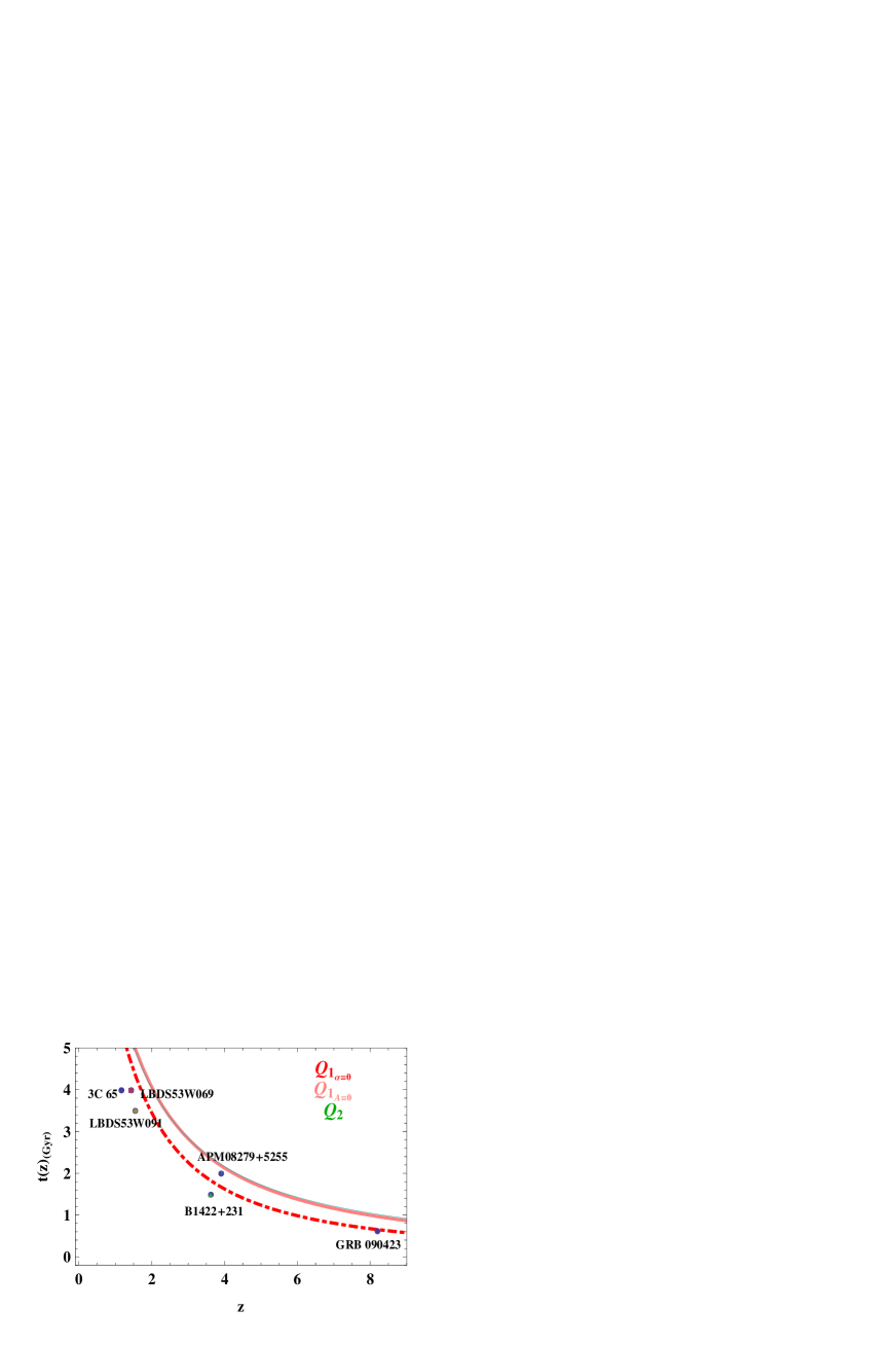
Now we are going to pay attention to the so-called “crisis of the age” in cosmology, which refers to the problem of having a universe younger than its constituents, and to its use to constrain cosmological models. This issue appears to have been noticed for the first time by Komossa et al. Komossa:2002cn , in the context of a matter dominated FRW universe and the use of abundance ratio of as cosmic clock. Moreover, the X-ray results of Hasinger et al. on the broad absorption line (BAL) quasar APM at redshift , that is, the high ratio (equivalent to a 3 Gyr old object), imply that SN Ia are involved Hasinger:2002wg , because of the inability to obtain these ratios in SN II. The introduction of dark energy alone does not remove the problem with this quasar and in Wang:2008te it has been shown that the interaction between dark matter and dark energy needs to be taken into account. Also, in the context of the holographic models Cui:2010dr , it has been achieved that to alleviate the problem, the interaction used must involve not only the dark holographic energy but also spatial curvature. The new agegraphic dark energy (NADE) models that include interactions between DE and DM (for example with and ) as in Li:2010ak have been able to accommodate this annoying object that has eluded be tamed in a huge variety of proposals Alcaniz:1999kr ; Friaca:2005ba ; Alcaniz:2003fy ; Yang:2009ae ; Wang:2010su ; Dantas:2006dy ; Capozziello:2007gr ; Movahed:2007cs ; Movahed:2007ie ; Movahed:2007ps ; Pires:2006rd ; Rahvar:2006tm ; Tong:2009mu ; Wei:2007ig ; Zhang:2007ps ; Duran:2010ky ; Forte:2012ww . Regardless of curvature, it seems still possible to alleviate the problem caused by the OHRO at , Duran:2010hi , but the age problem becomes serious when we consider the age of the universe at high redshift and it is a good test to be applied to the models proposed. To that end, we use some old high redshift objects (OHROs) discovered, for instance, the 3.5 Gyr old galaxy LBDS 53W091 Dunlop:1996mp ; Spinrad:1997md at redshift , the 4.0 Gyr old galaxy LBDS 53W069 Dunlop:1998tm at redshift , the 4.0 Gyr old radio galaxy 3C 65 at StocktonKelloggRidgway LacyRawlingsEalesDunlop , the high redshift quasar B1422+231 at Yoshii:1998bw whose best-fit age is 1.5 Gyr, besides of the aforementioned old quasar APM 08279+5255 at with 3.0 Gyr. To assure the robustness of our analysis, we use the 0.63 Gyr gamma-ray burst GRB 090423, at Tanvir:2009zz ; Salvaterra:2009ey detected by the Burst Alert Telescope (BAT) on the Swift satellite 18 on 23 April 2009. This is well beyond the redshift of the most distant spectroscopically confirmed galaxy () and quasar (). These OHRO’s are not the only ones available to qualify our interactions. In a recent work Balestra:2013gra , the VIMOS/VLT observations providing a spectroscopic confirmation at for a galaxy quintuply imaged by the Frontier Fields cluster RXC . These results, together with those recently presented by Monna:2013eia , suggest that this magnified, distant galaxy is a young with age less than 0.3 Gyr. In the future, through campaigns such as the Hubble Ultra Deep Field Ellis:2012bh we could obtain confirmation of the existence of other sources at redshift 8.5 to 12 whose estimated ages allow us to improve this comparison. In Fig.:25 the curves of time-redshift relation with best-fit parameters for the three models studied, are compared among themselves and with the old high redshift objects (OHROs). The milestones considered are old ratio galaxy 3C 65, old galaxy LBDS , old galaxy LBDS , high redshift quasar B, old quasar APM and the most distant GRB . It is observed that the crisis of cosmological age is solved for models with interactions and but not for those with interaction.
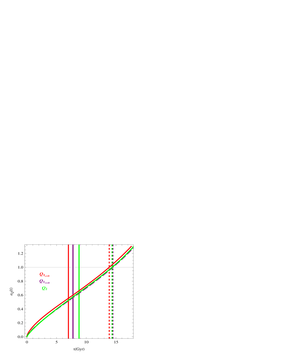
The parametric curves for the factor of scale of each models considered, drawn in Fig.:26, allow us to observe that all the interactions drive universes not accelerated in the remote past which effect their transitions to accelerated regime at different times (the saddle points marked with solid lines). The youngest universe ( in red) begins its acceleration about 7 Gyr after the Big Bang (BB) and of the other two, the oldest ( in purple) starts its transition before the other. The most delayed ( in green), starts its transition only after 10 Gyr from the BB. The horizontal line marks the present epoch, that is, the age of the universe , which for all the models is lower than 15 Gyr. According to the results of Table 3, the acceleration of the universe may have started between 7 and 9 Gyr after the Big Bang. Complementarily we can use the look back time of the beginning of that transition. The look-back time
is observationally estimated as the difference between the present day age of the universe and the age of a given object at redshift z Capozziello:2004jy Dalal:2001dt . The results correspond to an interval between 5.56 and 6.87 Gyr ago and agree with SN Ia observations, at approximately 6 billion light years ago, realized by two independent groups, led by S. Perlmutter and by B. Schmidt and A. Riess respectively, that revealed the acceleration of the universe (for what they got the Nobel prize in Physics 2011) Perlmutter:1998np ; Riess:1998cb .
V Conclusions
We studied three scenarios, with interactions in the dark sector which are able to change sign along the cosmological evolution, independently of the deceleration parameter and of the ratio of energy densities. We obtained the general solutions for each model, to which we added a material self preserved component. The models were statistically analyzed using the Hubble function and Tables 1-3 summarize the results for the best-fit models for each interaction. The couplings generate DM at the cost of DE, at early times, except in the second one, , where the opposite happens. The change of sign for each interaction is produced inside the interval of redshifts , which is consistent with the results of Cai Su, (), for cases as ours where . Table 1 contains the values of the coupling constants and of the equations of state of interactive and non interactive fluids, and the current value of the Hubble parameter. Table 2 consigns the current magnitudes of the interactions, of density parameters, of the deceleration parameter, the effective equation of state of dark energy and of the ratio of energy densities of the dark sector. In it, we can see the magnitude of the density parameter of dark energy at the BBN epoch and also the different redshifts: of the transitions to the accelerated regime, of the change of sign by the interactions and those for which the dark ratio is 1, used to qualify the merit of the interaction in alleviating the coincidence problem. Table 3 lists the age of the universe, the time since the BB to the beginnings of the transition to the accelerated regimen and the look back time of these beginnings. Moreover, it describes the CL for the coupling parameters or and and the ranges of variation for the transition redshift, for the current effective EoS of dark energy and for the current density parameter of total material component when the coupling constants vary within their CL. In the last two columns, Table 3 shows the qualifications of the interactions with respect to the coincidence problem and their success or failure with respect to the solution of the cosmological age crisis. All models correspond to decelerated universes at early times, which show acceleration at present time and change the direction of energy flows at redshifts consistent with the results of Cai Su. The confrontations of the distance modulus or of the Hubble function have not been adequate to test the three models and therefore we have appealed to the analysis of the values of EDE, and to the comparisons of time-redshift relations and parametric curves of the scale factors.
| Best Fit Parameters | Best Fit | ||||||||||
| Coupling constants | Model | ||||||||||
| 1 | 1 | 0 | 0.225 | 71.81 | 17.1474 | 0.816543 | CDM + Dust | ||||
| 1 | 1.2 | 0 | 0.04 | 71.42 | 17.7573 | 0.845586 | WDM + Dust | ||||
| 1 | 1 | 0 | 0.01 | 70.64 | 18.6807 | 0.889524 | CDM + Dust | ||||
| 0.03 | 0.004 | 0.771 | 0.225 | 0.229 | 0 | 0.297 | -0.656 | -1.04 | 0.805 | 1.19 | 0.443 | |
| - 0.20 | 0.13 | 0.83 | 0.04 | 0.170 | 0.236 | -0.7 | -0.763 | 0.772 | 0.48 | 0.7 | ||
| 0.45 | 0.124 | 0.866 | 0.01 | 0.134 | 0.155 | -0.8 | -1.514 | 0.570 | 0.5 | 0.3 |
| look-back | CL for | CL for | quality | solve | ||||||
| since BB | time | or | or | () | crisis | |||||
| [Gyr] | [Gyr] | [Gyr] | of age? | |||||||
| 6.87 | [-0.37,0.61] | [-3.9,7.3] | [0.74,0.89] | [-1.45,-0.95] | [0,0.3] | 33.13% | NO | |||
| 6.71 | [-1.86,-0.54] | [-0.022,0.337] | [0.6,0.9] | [-0.91,0.735] | [0,0.24] | 43.63% | YES | |||
| 5.57 | [0.33,1.87] | [0.515,1.650] | [0.45,0.65] | [-2.29,-1.045] | [0,0.3] | 24.03% | YES |
The most successful of the three interactions has proven to be that maintains appropriate residual value of the density parameter of dark energy at early times and get fit all controversial OHRO’s for flat FRW cosmologies, besides having the best factor quality. All these universes are aged below 15 Gyr and their look back times to the transition to the accelerated regime are around 6 Gyr, consistent with the results of Perlmutter, Schmidt and Riess. Notably, the difference observed in the saddle points of the parametric curves of the factor of scale, could make an interesting way to discriminate between these models if the transition redshift got determined with sufficient accuracy.
References
- (1) A. G. Riess et al. [Supernova Search Team Collaboration], Astron. J. 116, 1009 (1998) http://arxiv.org/abs/astroph/9805201; S. Perlmutter et al. [Supernova Cosmology Project Collaboration], Astrophys. J. 517, 565 (1999) [astro-ph/9812133]. http://arxiv.org/abs/astroph/9812133
- (2) M. Tegmark et al. [SDSS Collaboration], Phys. Rev. D 69, 103501 (2004); K. Abazajian et al. [SDSS Collaboration], Astron. J. 128, 502 (2004) http://arxiv.org/abs/astroph/0403325; K. Abazajian et al. [SDSS Collaboration], Astron. J. 129, 1755 (2005) http://arxiv.org/abs/astroph/0410239.
- (3) D. N. Spergel et al. [WMAP Collaboration], Astrophys. J. Suppl. 148, 175 (2003) http://arxiv.org/abs/astroph/0302209.
- (4) V. Sahni and A. A. Starobinsky, Int. J. Mod. Phys. D 9, 373 (2000) http://arxiv.org/abs/astroph/9904398; P. J. E. Peebles and B. Ratra, Rev. Mod. Phys. 75, 559 (2003) http://arxiv.org/abs/astroph/0207347; V. Sahni, Lect. Notes Phys. 653, 141 (2004) http://arxiv.org/abs/astroph/0403324; E. J. Copeland, M. Sami and S. Tsujikawa, Int. J. Mod. Phys. D 15, 1753 (2006) http://arxiv.org/abs/hep-th/0603057; J. Frieman, M. Turner and D. Huterer, Ann. Rev. Astron. Astrophys. 46, 385 (2008) http://arxiv.org/abs/0803.0982; S. ’i. Nojiri and S. D. Odintsov, Phys. Rept. 505, 59 (2011) http://arxiv.org/abs/1011.0544]; M. Li, X. -D. Li, S. Wang and Y. Wang, Commun. Theor. Phys. 56, 525 (2011) http://arxiv.org/abs/1103.5870.
- (5) C. Wetterich, Nucl. Phys. B 302, 668 (1988); B. Ratra and P. J. E. Peebles, Phys. Rev. D 37, 3406 (1988).
- (6) P. J. E. Peebles and B. Ratra, Rev. Mod. Phys. 75, 559 (2003) http://arxiv.org/abs/astroph/0207347.
- (7) E. W. Kolb, S. Matarrese and A. Riotto, New J. Phys. 8, 322 (2006) http://arxiv.org/abs/astroph/0506534.
- (8) J. R. Ellis, S. Kalara, K. A. Olive and C. Wetterich, Phys. Lett. B 228, 264 (1989); C. Wetterich, Astron. Astrophys. 301, 321 (1995) http://arxiv.org/abs/hep-th/9408025; L. Amendola, Phys. Rev. D 62, 043511 (2000) http://arxiv.org/abs/astroph/9908023; M. Gasperini, F. Piazza and G. Veneziano, Phys. Rev. D 65, 023508 (2002) http://arxiv.org/abs/gr-qc/0108016.
- (9) J. A. Casas, J. Garcia-Bellido and M. Quiros, Class. Quant. Grav. 9, 1371 (1992) http://arxiv.org/abs/hep-ph/9204213; G. W. Anderson and S. M. Carroll, In *Ambleside 1997, Particle physics and the early universe* 227-229 http://arxiv.org/abs/astroph/9711288. N. Bartolo and M. Pietroni, Phys. Rev. D 61, 023518 (2000) http://arxiv.org/abs/hep-ph/9908521; M. Pietroni, Phys. Rev. D 67, 103523 (2003) http://arxiv.org/abs/hep-ph/0203085; L. P. Chimento, A. S. Jakubi, D. Pavon and W. Zimdahl, Phys. Rev. D 67, 083513 (2003) http://arxiv.org/abs/astroph/0303145; L. P. Chimento, M. I. Forte and G. M. Kremer, Gen. Rel. Grav. 41, 1125 (2009) http://arxiv.org/abs/0711.2646; L. P. Chimento, M. I. Forte and M. G. Richarte, Mod. Phys. Lett. A 28, 1250235 (2013) http://arxiv.org/abs/1106.0781; C. S. Rhodes, C. van de Bruck, P. .Brax and A. C. Davis, Phys. Rev. D 68, 083511 (2003) http://arxiv.org/abs/astroph/0306343; G. R. Farrar and P. J. E. Peebles, Astrophys. J. 604, 1 (2004) http://arxiv.org/abs/astroph/0307316; A. Gromov, Y. .Baryshev and P. Teerikorpi, Astron. Astrophys. 415, 813 (2004) http://arxiv.org/abs/astroph//0209458; R. Mainini and S. A. Bonometto, Phys. Rev. Lett. 93, 121301 (2004) http://arxiv.org/abs/astroph/0406114.
- (10) X. -m. Chen, Y. Gong, E. N. Saridakis, Y. Gong and E. N. Saridakis, http://arxiv.org/abs/1111.6743.
- (11) O. Bertolami, F. Gil Pedro and M. Le Delliou, Phys. Lett. B 654, 165 (2007) http://arxiv.org/abs/astroph/0703462; O. Bertolami, F. G. Pedro and M. Le Delliou, Gen. Rel. Grav. 41, 2839 (2009) http://arxiv.org/abs/0705.3118; M. Le Delliou, O. Bertolami and F. Gil Pedro, AIP Conf. Proc. 957, 421 (2007) http://arxiv.org/abs/0709.2505; O. Bertolami, F. Gil Pedro and M. Le Delliou, EAS Publ. Ser. 30, 161 (2008) http://arxiv.org/abs/0801.0201.
- (12) E. Abdalla, L. R. W. Abramo, L. Sodre, Jr. and B. Wang, Phys. Lett. B 673, 107 (2009) http://arxiv.org/abs/0710.1198.
- (13) J. -H. He, B. Wang and P. Zhang, Phys. Rev. D 80, 063530 (2009) http://arxiv.org/abs/0906.0677.
- (14) Z. -K. Guo, N. Ohta and S. Tsujikawa, Phys. Rev. D 76, 023508 (2007) http://arxiv.org/abs/astroph/0702015.
- (15) M. Quartin, M. O. Calvao, S. E. Joras, R. R. R. Reis and I. Waga, JCAP 0805, 007 (2008) http://arxiv.org/abs/0802.0546.
- (16) D. Pavon and B. Wang, Gen. Rel. Grav. 41, 1 (2009) http://arxiv.org/abs/0712.0565.
- (17) S. H. Pereira and J. F. Jesus, Phys. Rev. D 79, 043517 (2009) http://arxiv.org/abs/0811.0099.
- (18) J. A. S. Lima and S. H. Pereira, Phys. Rev. D 78, 083504 (2008) http://arxiv.org/abs/0801.0323.
- (19) S. H. Pereira and J. A. S. Lima, Phys. Lett. B 669, 266 (2008) http://arxiv.org/abs/0806.0682.
- (20) S. H. Pereira, http://arxiv.org/abs/0806.3701.
- (21) G. Olivares, F. Atrio-Barandela and D. Pavon, Phys. Rev. D 77, 103520 (2008) http://arxiv.org/abs/0801.4517.
- (22) R. -G. Cai and Q. Su, Phys. Rev. D 81, 103514 (2010) http://arxiv.org/abs/0912.1943.
- (23) H. Wei, Commun. Theor. Phys. 56, 972 (2011) http://arxiv.org/abs/1010.1074; C. -Y. Sun and R. -H. Yue, Phys. Rev. D 85, 043010 (2012) http://arxiv.org/abs/1009.1214; Y. D. Xu and Z. G. Huang, Astrophys. Space Sci. 343, 807 (2013); Y. D. Xu and X. H. Zhai, Astrophys. Space Sci. 345, 381 (2013).
- (24) Press, W.H., et al., Numerical Recipes in C. Cambridge University Press, Cambridge (1997)
- (25) D. Stern, R. Jimenez, L. Verde, M. Kamionkowski and S. A. Stanford, JCAP 1002 (2010) 008 http://arxiv.org/abs/0907.3149.
- (26) J. Simon, L. Verde and R. Jimenez, Phys. Rev. D 71, 123001 (2005) http://arxiv.org/abs/astroph/0412269.
- (27) K. Liao, Z. Li, J. Ming and Z. -H. Zhu, Phys. Lett. B 718, 1166 (2013) http://arxiv.org/abs/1212.6612.
- (28) O. Farooq and B. Ratra, http://arxiv.org/abs/1301.5243.
- (29) M. Moresco, L. Verde, L. Pozzetti, R. Jimenez and A. Cimatti, JCAP 1207, 053 (2012) http://arxiv.org/abs/1201.6658.
- (30) A. G. Riess et al., Astrophys. J. 699 (2009) 539 http://arxiv.org/abs/1011.1982.
- (31) L. Samushia and B. Ratra, Astrophys. J. 650, L5 (2006) http://arxiv.org/abs/astroph/0607301.
- (32) H. Wei and S. N. Zhang, Phys. Lett. B 644, 7 (2007) http://arxiv.org/abs/astroph/0609597.
- (33) R. Lazkoz and E. Majerotto, JCAP 0707, 015 (2007) http://arxiv.org/abs/0704.2606.
- (34) H. Lin, C. Hao, X. Wang, Q. Yuan, Z. -L. Yi, T. -J. Zhang and B. -Q. Wang, Mod. Phys. Lett. A 24, 1699 (2009) http://arxiv.org/abs/0804.3135.
- (35) S. Cao, N. Liang and Z. -H. Zhu, http://arxiv.org/abs/1105.6274.
- (36) D. G. Figueroa, L. Verde and R. Jimenez, JCAP 0810, 038 (2008) http://arxiv.org/abs/0807.0039.
- (37) M. Seikel, S. Yahya, R. Maartens and C. Clarkson, http://arxiv.org/abs/1205.3431.
- (38) R. C. Santos, F. E. Silva and J. A. S. Lima, http://arxiv.org/abs/1103.4988.
- (39) S. del Campo, R. Herrera and D. Pavon, J. Phys. Conf. Ser. 229, 012012 (2010).
- (40) A. Aviles, A. Bravetti, S. Capozziello and O. Luongo, http://arxiv.org/abs/1210.5149.
- (41) N. Said, C. Baccigalupi, M. Martinelli, A. Melchiorri and A. Silvestri, http://arxiv.org/abs/1303.4353.
- (42) W. Fang, W. Hu and A. Lewis, Phys. Rev. D 78, 087303 (2008) http://arxiv.org/abs/0808.3125.
- (43) P. A. R. Ade et al. [Planck Collaboration], http://arxiv.org/abs/1303.5076.
- (44) J. V. Cunha and J. A. S. Lima, Mon. Not. Roy. Astron. Soc. 390, 210 (2008) http://arxiv.org/abs/0805.1261.
- (45) L. P. Chimento, M. I. Forte and M. G. Richarte, Mod. Phys. Lett. A 28, 1250235 (2013) http://arxiv.org/abs/1106.0781.
- (46) L. P. Chimento, M. Forte and M. G. Richarte, Eur. Phys. J. C 73, 2285 (2013) http://arxiv.org/abs/1301.2737.
- (47) L. Chimento and M. I. Forte, Phys. Lett. B 666, 205 (2008) http://arxiv.org/abs/0706.4142.
- (48) L. P. Chimento, M. I. Forte and G. M. Kremer, Gen. Rel. Grav. 41, 1125 (2009) http://arxiv.org/abs/0711.2646.
- (49) M. I. Forte and M. G. Richarte, http://arxiv.org/abs/1206.1073.
- (50) B. Carter, Lect. Notes Math. 1385, 1 (1989).
- (51) T. Harko and F. Lobo, Astropart.Phys.35,547-551(2012) http://arxiv.org/abs/1104.2674.
- (52) S. Bharadwaj and S. Kar, Phys. Rev. D 68,023516(2003) http://arxiv.org/abs/0304504.
- (53) K. Y. Su and P. Chen, Phys. Rev. D 79,128301(2009) http://arxiv.org/abs/0905.2084.
- (54) C. J. Saxton and I. Ferreras, Month. Not. R. Astron. Soc. 405,77(2010) http://arxiv.org/abs/1002.0845.
- (55) E. A. Lim, I. Sawicki and A. Vikman, JCAP 1005, 012 (2010) http://arxiv.org/abs/1003.5751.
- (56) B. Moore, T. R. Quinn, F. Governato, J. Stadel and G. Lake, Mon. Not. Roy. Astron. Soc. 310, 1147 (1999) http://arxiv.org/abs/astroph/9903164.
- (57) P. Bode, J. P. Ostriker and N. Turok, Astrophys. J. 556, 93 (2001) http://arxiv.org/abs/astroph/0010389.
- (58) V. Avila-Reese, P. Colin, O. Valenzuela, E. D’Onghia and C. Firmani, Astrophys. J. 559, 516 (2001) http://arxiv.org/abs/astroph/0010525.
- (59) J. J. Dalcanton and C. J. Hogan, Astrophys. J. 561, 35 (2001) http://arxiv.org/abs/astroph/0004381.
- (60) D. Boyanovsky and J. Wu, Phys. Rev. D 83, 043524 (2011) http://arxiv.org/abs/1008.0992.
- (61) C. Destri, H. J. de Vega and N. G. Sanchez, New Astron. 22, 39 (2013) http://arxiv.org/abs/1204.3090.
- (62) B. Feng, X. -L. Wang and X. -M. Zhang, Phys. Lett. B 607, 35 (2005) http://arxiv.org/abs/astroph/0404224; D. Huterer and A. Cooray, Phys. Rev. D 71, 023506 (2005) http://arxiv.org/abs/astroph/0404062; H. Zhang, http://arxiv.org/abs/0909.3013; Z. -K. Guo, Y. -S. Piao, X. -M. Zhang and Y. -Z. Zhang, Phys. Lett. B 608, 177 (2005) http://arxiv.org/abs/astroph/0410654; H. Wei, R. -G. Cai and D. -F. Zeng, Class. Quant. Grav. 22, 3189 (2005) http://arxiv.org/abs/hep-th/0501160; Y. -F. Cai, E. N. Saridakis, M. R. Setare and J. -Q. Xia, Phys. Rept. 493, 1 (2010) http://arxiv.org/abs/0909.2776; M. R. Setare, Phys. Lett. B 641, 130 (2006) http://arxiv.org/abs/hep-th/0611165; H. Mohseni Sadjadi and M. Alimohammadi, Phys. Rev. D 74, 043506 (2006) http://arxiv.org/abs/gr-qc/0605143; P. Astier et al. [SNLS Collaboration], Astron. Astrophys. 447, 31 (2006) http://arxiv.org/abs/astroph/0510447; R. Lazkoz, G. Leon and I. Quiros, Phys. Lett. B 649, 103 (2007) http://arxiv.org/abs/astroph/0701353; L. P. Chimento, M. I. Forte, R. Lazkoz and M. G. Richarte, Phys. Rev. D 79, 043502 (2009) http://arxiv.org/abs/0811.3643; M. Alimohammadi and H. M. Sadjadi, Phys. Lett. B 648, 113 (2007) http://arxiv.org/abs/gr-qc/0608016.
- (63) J. A. S. Lima, J. F. Jesus, R. C. Santos and M. S. S. Gill, http://arxiv.org/abs/1205.4688.
- (64) J. V. Cunha, Phys. Rev. D 79, 047301 (2009) http://arxiv.org/abs/0811.2379.
- (65) D. -Z. Liu, S. Yuan, Y. Lu and T. -J. Zhang, http://arxiv.org/abs/1208.4665.
- (66) D. Huterer and A. Cooray, Phys. Rev. D 71, 023506 (2005) http://arxiv.org/abs/astroph/0404062;
- (67) R. Kessler, A. Becker, D. Cinabro, J. Vanderplas, J. A. Frieman, J. Marriner, T. MDavis and B. Dilday et al., Astrophys. J. Suppl. 185, 32 (2009) http://arxiv.org/abs/0908.4274.
- (68) M. Sullivan, J. Guy, A. Conley, N. Regnault, P. Astier, C. Balland, S. Basa and R. G. Carlberg et al., Astrophys. J. 737, 102 (2011) http://arxiv.org/abs/1104.1444.
- (69) N. Suzuki, D. Rubin, C. Lidman, G. Aldering, R. Amanullah, K. Barbary, L. F. Barrientos and J. Botyanszki et al., Astrophys. J. 746, 85 (2012) http://arxiv.org/abs/1105.3470.
- (70) S. Nesseris and L. Perivolaropoulos, JCAP 0701, 018 (2007) http://arxiv.org/abs/astroph/0610092.
- (71) C. Wetterich, Phys. Lett. B 594, 17 (2004) http://arxiv.org/abs/astroph/0403289.
- (72) P. G. Ferreira and M. Joyce, Phys. Rev. D 58, 023503 (1998) http://arxiv.org/abs/astroph/9711102.
- (73) R. H. Cyburt, B. D. Fields, K. A. Olive and E. Skillman, Astropart. Phys. 23, 313 (2005) http://arxiv.org/abs/astroph/0408033.
- (74) E. Calabrese, D. Huterer, E. V. Linder, A. Melchiorri and L. Pagano, Phys. Rev. D 83, 123504 (2011) http://arxiv.org/abs/1103.4132.
- (75) J. L. Sievers, R. A. Hlozek, M. R. Nolta, V. Acquaviva, G. E. Addison, P. A. R. Ade, P. Aguirre and M. Amiri et al., http://arxiv.org/abs/1301.0824.
- (76) C. LReichardt, R. de Putter, O. Zahn and Z. Hou, Astrophys. J. 749, L9 (2012) http://arxiv.org/abs/1110.5328.
- (77) M. Doran, J. -M. Schwindt and C. Wetterich, Phys. Rev. D 64, 123520 (2001) http://arxiv.org/abs/astroph/0107525.
- (78) R. R. Caldwell, M. Doran, C. M. Mueller, G. Schafer and C. Wetterich, Astrophys. J. 591, L75 (2003) http://arxiv.org/abs/astroph/0302505.
- (79) E. Calabrese, R. de Putter, D. Huterer, E. V. Linder and A. Melchiorri, Phys. Rev. D 83, 023011 (2011) http://arxiv.org/abs/1010.5612.
- (80) Z. Hou, C. L. Reichardt, K. T. Story, B. Follin, R. Keisler, K. A. Aird, B. A. Benson and L. E. Bleem et al., http://arxiv.org/abs/1212.6267.
- (81) V. Pettorino, L. Amendola and C. Wetterich, Phys. Rev. D 87, 083009 (2013) http://arxiv.org/abs/1301.5279.
- (82) C. L. Bennett et al. [WMAP Collaboration], http://arxiv.org/abs/1212.5225.
- (83) E. Calabrese, E. Menegoni, C. J. A. P. Martins, A. Melchiorri and G. Rocha, “Constraining Variations in the Fine Structure Constant in the presence of Early Dark Energy,” Phys. Rev. D 84, 023518 (2011) http://arxiv.org/abs/1104.0760.
- (84) L. Hollenstein, D. Sapone, R. Crittenden and B. M. Schaefer, JCAP 0904, 012 (2009) http://arxiv.org/abs/0902.1494.
- (85) K. Cahill, http://arxiv.org/abs/1308.6001.
- (86) S. Komossa and G. Hasinger, http://arxiv.org/abs/astroph/0207321.
- (87) G. Hasinger, N. Schartel and S. Komossa, Astrophys. J. 573, L77 (2002) http://arxiv.org/abs/astroph/0207005.
- (88) S. Wang and Y. Zhang, Phys. Lett. B 669, 201 (2008) http://arxiv.org/abs/0809.3627.
- (89) J. Cui and X. Zhang, Phys. Lett. B 690, 233 (2010) http://arxiv.org/abs/1005.3587.
- (90) Y. Li, J. Ma, J. Cui, Z. Wang and X. Zhang, Sci. China Phys. Mech. Astron. G 54, no. issue, 1367 (2011) http://arxiv.org/abs/1011.6122.
- (91) J. S. Alcaniz and J. A. S. Lima, Astrophys. J. 521, L87 (1999) http://arxiv.org/abs/astroph/9902298.
- (92) A. Friaca, J. Alcaniz and J. A. S. Lima, Mon. Not. Roy. Astron. Soc. 362, 1295 (2005) http://arxiv.org/abs/astroph/0504031.
- (93) J. S. Alcaniz, J. A. S. Lima and J. V. Cunha, Mon. Not. Roy. Astron. Soc. 340, L39 (2003) http://arxiv.org/abs/astroph/0301226.
- (94) R. -J. Yang and S. N. Zhang, Mon. Not. Roy. Astron. Soc. 407, 1835 (2010) http://arxiv.org/abs/0905.2683.
- (95) S. Wang, X. -D. Li and M. Li, Phys. Rev. D 82, 103006 (2010) http://arxiv.org/abs/1005.4345.
- (96) M. A. Dantas, J. S. Alcaniz, D. Jain and A. Dev, Astron. Astrophys. 467, 421 (2007) http://arxiv.org/abs/astroph/0607060.
- (97) S. Capozziello, P. K. S. Dunsby, E. Piedipalumbo and C. Rubano, http://arxiv.org/abs/0706.2615.
- (98) S. Capozziello, V. F. Cardone, M. Funaro and S. Andreon, Phys. Rev. D 70, 123501 (2004) http://arxiv.org/abs/astroph/0410268.
- (99) N. Dalal, K. Abazajian, E. E. Jenkins and A. V. Manohar, Phys. Rev. Lett. 87, 141302 (2001) http://arxiv.org/abs/astroph/0105317.
- (100) M. S. Movahed, S. Baghram and S. Rahvar, Phys. Rev. D 76, 044008 (2007) http://arxiv.org/abs/0705.0889.
- (101) M. S. Movahed, M. Farhang and S. Rahvar, Int. J. Theor. Phys. 48, 1203 (2009) http://arxiv.org/abs/astroph/0701339.
- (102) M. S. Movahed and S. Ghassemi, Phys. Rev. D 76, 084037 (2007) http://arxiv.org/abs/0705.3894.
- (103) N. Pires, Z. -H. Zhu and J. S. Alcaniz, Phys. Rev. D 73, 123530 (2006) http://arxiv.org/abs/astroph/0606689.
- (104) S. Rahvar and M. S. Movahed, Phys. Rev. D 75, 023512 (2007) http://arxiv.org/abs/astroph/0604206.
- (105) M. -L. Tong and Y. Zhang, Phys. Rev. D 80, 023503 (2009) http://arxiv.org/abs/0906.3646.
- (106) H. Wei and S. N. Zhang, Phys. Rev. D 76, 063003 (2007) http://arxiv.org/abs/0707.2129.
- (107) Y. Zhang, H. Li, X. Wu, H. Wei and R. -G. Cai, http://arxiv.org/abs/0708.1214.
- (108) I. Duran and D. Pavon, Phys. Rev. D 83, 023504 (2011) http://arxiv.org/abs/1012.2986.
- (109) I. Duran, D. Pavon and W. Zimdahl, JCAP 1007, 018 (2010) http://arxiv.org/abs/1007.0390.
- (110) J. Dunlop, J. Peacock, H. Spinrad, A. Dey, R. Jimenez, D. Stern and R. Windhorst, Nature 381, 581 (1996).
- (111) H. Spinrad, A. Dey, D. Stern, J. Dunlop, J. Peacock, R. Jimenez and R. Windhorst, Astrophys. J. 484, 581 (1997) http://arxiv.org/abs/astroph/9702233.
- (112) J. Dunlop, The Most Distant Radio Galaxies, ed. by J.J.A. Rottgering, P. Best, M.D. Lehnert (Kluwer Academic, Dordrecht,1999), p. 71 http://arxiv.org/abs/astroph/9801114.
- (113) A. Stockton, M. Kellogg and S. E. Ridgway, Astrophys. J. 443, L69 (1995).
- (114) M. Lacy, S. Rawlings, S. Eales,and J. S. Dunlop, Mon. Not. Roy. Astron. Soc. 273, 821 (1995)
- (115) Y. Yoshii, T. Tsujimoto and K. Kawara, Astrophys. J. 507, L113 (1998) http://arxiv.org/abs/astroph/9809047.
- (116) N. R. Tanvir, D. B. Fox, A. J. Levan, E. Berger, K. Wiersema, J. P. U. Fynbo, A. Cucchiara and T. Kruhler et al., Nature 461, 1254 (2009) http://arxiv.org/abs/0906.1577.
- (117) R. Salvaterra, M. Della Valle, S. Campana, G. Chincarini, S. Covino, P. D’Avanzo, A. Fernandez-Soto and C. Guidorzi et al., http://arxiv.org/abs/0906.1578.
- (118) I. Balestra, E. Vanzella, P. Rosati, A. Monna, C. Grillo, M. Nonino, A. Mercurio and A. Biviano et al., http://arxiv.org/abs/1309.1593.
- (119) A. Monna, S. Seitz, N. Greisel, T. Eichner, N. Drory, M. Postman, A. Zitrin and D. Coe et al., http://arxiv.org/abs/1308.6280.
- (120) R. SEllis, R. JMcLure, J. SDunlop, B. ERobertson, Y. Ono, M. ASchenker, A. Koekemoer and R. A ABowler et al., Astrophys. J. 763, L7 (2013) http://arxiv.org/abs/1211.6804.
- (121) S. Perlmutter et al. [Supernova Cosmology Project Collaboration], Astrophys. J. 517, 565 (1999) http://arxiv.org/abs/astro-ph/9812133.
- (122) A. G. Riess et al. [Supernova Search Team Collaboration], Astron. J. 116, 1009 (1998) http://arxiv.org/abs/astro-ph/9805201.