The Landau–Zener Problem with Decay and with Dephasing

Abstract

Two aspects of the classic two-level Landau–Zener (LZ) problem are considered. First, we address the LZ problem when one or both levels decay, i.e., $\varepsilon_{j}(t)\to\varepsilon_{j}(t)-i\Gamma_{j}/2$. We find that if the system evolves from an initial time $-T$ to a final time $+T$ such that $|\varepsilon_{1}(\pm T)-\varepsilon_{2}(\pm T)|$ is not too large, the LZ survival probability of a state $|j\rangle$ can increase with increasing decay rate of the other state $|i\neq j\rangle$. This surprising result occurs because the decay results in crossing of the two eigenvalues of the instantaneous non-Hermitian Hamiltonian. On the other hand, if $|\varepsilon_{1}(\pm T)-\varepsilon_{2}(\pm T)|\to\infty$ as $T\to\infty$, the probability is independent of the decay rate. These results are based on analytic solutions of the time-dependent Schrödinger equations for two cases: (a) the energy levels depend linearly on time, and (b) the energy levels are bounded and of the form $\varepsilon_{1,2}(t)=\pm\varepsilon\tanh(t/{\cal T})$. Second, we study LZ transitions affected by dephasing by formulating the Landau–Zener problem with noise in terms of a Schrödinger-Langevin stochastic coupled set of differential equations. The LZ survival probability then becomes a random variable whose probability distribution is shown to behave very differently for long and short dephasing times. We also discuss the combined effects of decay and dephasing on the LZ probability.

I Introduction

The Landau–Zener (LZ) problem Landau_32 ; Zener_32 ; Stueckelberg_32 ; Majorana_32 has been the subject of intense study for over four score years. It has become a paradigm time-dependent two-level dynamical model that has been applied in many areas of quantum physics. Here we shall focus on two extensions of this classic problem. Let us first briefly remind the reader of the original LZ problem, since it serves as a starting point for the extensions. The LZ problem involves the evolution of the wave function of a coupled two-level system whose time-dependent energies, when uncoupled, cross at some time, say $t_{0}=0$ (see Fig. 1). The relevant physical quantity is the LZ probability, i.e., the modulus squared of one of the components of the wave function, as time $t\to\infty$, and it is of interest to determine its dependence on the coupling strength and on the rate of energy change with time.

In the original version of the problem Landau_32 ; Zener_32 ; Stueckelberg_32 ; Majorana_32 , the energy levels depend linearly on time. Two widely used forms, displayed in Figs. 1(a) and 1(b) are,

$$H_{1}(t)=\left(\!\!\begin{array}[]{cc}0&V\\ V&-\alpha t\end{array}\!\!\right),\quad H_{2}(t)=\frac{\alpha t}{2}\sigma_{z}+V\sigma_{x}=\left(\!\!\begin{array}[]{cc}\alpha t/2&V\\ V&-\alpha t/2\end{array}\!\!\right).$$ (1)

Here, $\sigma_{x},\sigma_{y}$ and $\sigma_{z}$ are the Pauli matrices, and $\alpha$ is the rate of unperturbed energy change. A unitary time-dependent transformation of $H_{1}(t)$ yields $H_{2}(t)$. Figure 1(a) plots the eigenvalues of $H_{1}(t)$ and Fig. 1(b) plots the diagonal elements and the instantaneous eigenvalues $E_{f,i}(t)=\pm\sqrt{(\alpha t/2)^{2}+V^{2}}$ of $H_{2}(t)$ versus time. As will be argued below, in the presence of level decay, it is useful to consider other models where, unlike the linear time-dependent levels, the dependence of the unperturbed levels $H_{ii}(t)$ on time are such that $H_{ii}(t)$ is bounded at all times. One such model is

$$H(t)=\begin{pmatrix}\varepsilon\tanh(t/{\cal T})&V\\ V&-\varepsilon\tanh(t/{\cal T})\end{pmatrix},$$ (2)

where $1/{\cal T}$ controls the rate of energy change near $t=0$.

The LZ problem can be stated as follows: what is the survival probability $P$ of finding the system in state $|1\rangle$ as $t\rightarrow\infty$, if it starts off in the state $|1\rangle$ as $t\rightarrow-\infty$ [see Fig. 1(b), where states $|1\rangle$ and $|2\rangle$ are the diabatic states, and $|i\rangle$ and $|f\rangle$ are the adiabatic states]. As $\alpha\to 0$, the adiabatic theorem ensures that the system stays in the initial adiabatic state $|i\rangle$. The original LZ problem can be formulated as follows: Let $P_{i}(\alpha,V)=\lim_{t\to\infty}|\psi_{i}(t)|^{2}$ denote the survival probability of state $i$ at large time. Find $P_{i}$ and analyze its dependence on $\alpha$ and $V$.

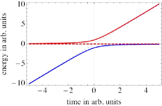
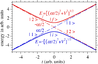
Figure 1: (Color online) (a) Eigenvalues of $H_{1}(t)$ in Eq. (1) (solid curves) and the diagonal Hamiltonian matrix elements (dashed lines), with $\alpha=-2$, $V=1$. (b) Eigenvalues of $H_{2}(t)$ in Eq. (1) (solid curves) and the diagonal Hamiltonian matrix elements (dashed lines), with $\alpha=2$, $V=1$.

In this paper we consider two extensions of the original problem which are of physical interest. First, we focus on the case where one or both of the energy levels decay. The motivation for studying the effects of level decay on the LZ probability is that decay occurs in many physical processes, including light-induced transitions between metastable states Burshtein_88 , collision-induced losses of laser-cooled atoms in magneto-optical traps Marcassa_93 ; Band_94 , photoassociative ionization collisions in a magneto-optical traps Bagnato_93 , and adiabatic fast passage in nuclear magnetic resonance population inversion processes in the presence of radio-frequency magnetic fields Hardy_86 , to mention a few.

Level decay can be modeled by letting the diagonal elements of the Hamiltonian acquire a time-independent negative imaginary part, ${\mathrm{Im}}[H_{ii}]=-\Gamma_{i}/2$, where $\Gamma_{i}/\hbar$ is the decay rate of level $i,\ (i=1,2)$. For example, consider the case where $H_{1}(t)$, Eq. (1), is modified such that the matrix element $H_{22}=-\alpha t-i\Gamma/2$. Transitions between decaying states were analyzed both using a master equation approach and by adding a decay term to the Hamiltonian in Ref. Burshtein_88 . Here we obtain analytic solutions using the latter method and analyze our results in terms of avoided level crossing in the complex energy plane.

In the absence of coupling, $V=0$ in Eq. (1), the corresponding diabatic wave function propagates as $\psi_{2}(t)=\exp[(-i(\alpha t-\alpha T-i\Gamma)(t+T)/2]\psi_{2}(-T)$. But with $V\neq 0$, the decay of level 2 affects the survival probability of level 1 in a non-trivial way, and we obtain the Landau–Zener problem with decay. The central goal of this problem is to determine the probability $P(T)=|\psi_{1}(T)|^{2}$ that the adiabatic state $\psi_{1}(T)$ is occupied in the far future, given the initial condition that in the far past it was fully occupied, $|\psi_{1}(-T)|^{2}=1$. The reason for insisting on a finite (albeit large) time $T$ will become evident below.

For the Hamiltonian $H_{1}(t)$ in Eq. (1), modified by adding ${\mathrm{Im}}[H_{22}]=-\Gamma/2$, the LZ problem with decay was addressed by Akulin and Schleich Akulin_Schleich_92 . The probability $P(\infty)$, is found to be independent of $\Gamma$ comment_AS . We show below that this result is due to the divergence of $|H_{11}(t)-H_{22}(t)|$ as $|t|\to\infty$, i.e., it is in some sense an artifact. One of our main goals is then to study models for the LZ problem with decay where $|H_{11}(t)-H_{22}(t)|$ is bounded as $|t|\to\infty$, and show that in this case, $P(T)$ does depend on $\Gamma$. Work on related problems has been reported in Refs. Band_94 ; Burshtein_88 ; Dridi_10 ; Dridi_12 ; Scala_11 ; Uzdin_12 ; Kocharovsky_77 ; Kocharovsky_rev ; Suominen_98 ; Vitanov_97 ; Moyer_01 ; Benderskii_04 ; Graefe_06 ; Schilling_06 ; Shore_06 ; Fainberg_07 ; Castro_08 , Refs. Gefen_87 ; Rammer ; Saito_07 consider a LZ transition for two states coupled to a bath of harmonic oscillators, and Refs. Rammer ; Saito_07 find that at zero temperature there is no influence of the environment on the transition probability, in a fashion similar to the Akulin and Schleich result Akulin_Schleich_92 .

The second extension considered here concerns the case where the LZ transition is affected by dephasing. Dephasing of a quantum system occurs due to interaction between the system and its environment. Examples include collisions of a particle with other particles, and interactions with environmental degrees of freedom such as an electromagnetic field that is random or stochastic. In the case of dephasing due to collisions with particles, each collision can have a random duration and a random strength; in the case of interactions with an environment, the many degrees of freedom of the environment (the “bath”) can randomly affect the phase of the wave function. This results in a time-dependent uncertainty $\delta(\varphi(t))$ in the phase of the wave function. At a time $t=\tau$ for which $\delta(\varphi(\tau))=2\pi$, interference is completely lost. Incorporation of dephasing in LZ transitions has been extensively studied Rammer ; Efrat1 ; Efrat2 ; Pokrovsky ; Avron . Dephasing processes occur in metals Aleiner_01 . Moreover, dephasing is important in atomic clock transitions ChangYeLukin_04 , in quantum information processes qc and in nuclear-spin-dependent ground-state dephasing of diamond nitrogen-vacancy centers NV . We treat such transitions using a Schrödinger-Langevin stochastic differential equation formalism vanKampenBook , and solve the time-dependent Schrödinger equation with a Gaussian white-noise stochastic term, and with Ornstein–Uhlenbeck noise. This enables us to study not only the averaged survival probability but also its distribution and its dependence on the strength of coupling between the system and the environment. As we shall see, the distribution in the strong coupling regime (short dephasing time) is very different from that in the weak coupling regime, both for white-noise and for Ornstein–Uhlenbeck noise.

The outline of the paper is as follows. Section II formulates the LZ problem with decay. In Sec. II.1 the problem is cast as a set of two uncoupled second order differential equations. This formalism is used to arrive at analytic solutions in Sec. II.2 for the time-dependent Schrödinger equations derived from $H_{1}(t)$ in Eq. (1) and in Sec. II.3 for the Hamiltonian in Eq. (2), properly modified to include decay terms. Section III presents numerical and analytical examples worked out with these Hamilonians. Section IV describes the dynamics of LZ when both levels decay. Section V considers LZ transitions with dephasing due to interaction with an environment. Finally, Sec. VI contains a summary and conclusion.

II The Landau–Zener problem with decay

In this section we formulate and solve the LZ problem with decay. The approach is to replace the set of two coupled first order differential equations by a set of two uncoupled second order differential equations. Analytic solutions of the time-dependent Schrödinger equations are obtained for $H_{1}(t)$ in Eq. (1), and for the Hamiltonian of Eq. (2), with the diagonal elements modified to have a time-independent negative imaginary part. The solutions of the resulting differential equations are obtained in terms of transcendental functions and expressions for the wave functions that satisfy the appropriate boundary conditions are presented.

II.1 Derivation of second order differential equations for $\psi_{i}(t)$

The most general form of the LZ problem is encoded in the time-dependent Schrd̈ingier equation for the two-component spinor $\psi=\binom{\psi_{1}(t)}{\psi_{2}(t)}$ that include also initial condition at time $t=-T$ for large $T$,

$$i\dot{\psi}=H\psi=\begin{pmatrix}Z_{1}(t)&V\\ V&Z_{2}(t)\end{pmatrix},\quad\psi_{1}(-T)=1,\ \ \psi_{2}(-T)=0.$$ (3)

Expressing $\psi_{2}(t)$ in terms of $\psi_{1}(t)$ by using the first equation, and substituting into the second equation we find,

$$\ddot{\psi}_{1}(t)+i[Z_{1}(t)+Z_{2}(t)]\dot{\psi}_{1}(t)+[V^{2}-Z_{1}(t)Z_{2}(t)+i\dot{Z}_{1}(t)]\psi_{1}(t)=0,\quad\psi_{1}(-T)=1,\ \ \dot{\psi}_{1}(-T)=-iZ_{1}(-T)~{}.$$ (4)

Both Hamiltonians in Eq. (1) can be written in the form of Eq. (3), and a diagonal time-dependent transformation can transform from one form to the other.

II.2 Solution of the Akulin-Schleich Version

Consider the Hamiltonian $H_{1}(t)$ in Eq. (1), modified to include an imaginary part in $H_{22}(t)$,

$$H=\begin{pmatrix}0&V\\ V&-\tfrac{1}{2}(\alpha t+i\Gamma)\end{pmatrix},$$ (5)

where for convenience we replace $\alpha\to\alpha/2$. Here $\alpha>0$ ($[\alpha]=$ energy/time), $V>0$ and $\Gamma>0$ are constants ($[V]=[\Gamma]=$ energy). It is useful to define a dimensionless time $\tau$, a dimensionless adiabaticity parameter $\lambda$, and a dimensionless decay parameter $\beta$. Restoring $\hbar$, these are defined as,

$$t\to\xi\tau\ \ (\xi\equiv\sqrt{\tfrac{\hbar}{2\alpha}},\ \ [\xi]=\mbox{time}),\quad\lambda\equiv\frac{V}{\sqrt{\alpha\hbar}},\quad\beta=\frac{\Gamma}{\sqrt{\alpha\hbar}}.$$ (6)

Renaming the dimensionless time to be $t$, instead of $\tau$, we obtain the dimensionless version of the Hamiltonian used in Ref. Akulin_Schleich_92 is

$${\cal H}(t)=\left(\!\!\begin{array}[]{cc}0&\ \ \ \lambda\\ \lambda&\ \ -\tfrac{1}{2}(t+i\beta)\end{array}\!\!\right)\equiv\left(\!\!\begin{array}[]{cc}0&\lambda\\ \lambda&z(t)\end{array}\!\!\right).$$ (7)

This is a special case of the $2\times 2$ Hamiltonian defined in Eq. (3) with $Z_{1}(t)=0$, and $Z_{2}(t)=z(t)\equiv-\tfrac{1}{2}(t+i\beta)$ and $V\to\lambda$. The time-dependent Schrödinger equations take the form,

$$i{\dot{\psi}}_{1}(t)=\lambda\psi_{2}(t),$$ (8a)

$$i{\dot{\psi}}_{2}(t)=\lambda\psi_{1}(t)+z(t)\psi_{2}(t).$$ (8b)

Employing the procedure detailed in arriving Eq. (4), the second-order differential equations for $\psi_{1}(t)$ and $\psi_{2}(t)$ are,

$$\ddot{\psi}_{1}-\tfrac{1}{2}(it-\beta)\dot{\psi}_{1}+\lambda^{2}\psi_{1}=0,$$ (9a)

$$\ddot{\psi}_{2}-\tfrac{1}{2}(it-\beta)\dot{\psi}_{2}+(\lambda^{2}-\tfrac{i}{2})\psi_{2}=0,$$ (9b)

with the initial conditions for $\psi_{1}(t)$ being,

$$\psi_{1}(-T)=1,\quad\dot{\psi}_{1}(-T)=-i\lambda\psi_{2}(-T)=0.$$ (10)

The most general solution of each second order differential equation is a linear combination of two basic solutions of the differential equations Eq. (9a) and Eq. (9b) given respectively as,

$$F_{11}(t)=D\left(-2i\lambda^{2},\tfrac{1}{2}(e^{i\frac{\pi}{4}}t+e^{i\frac{3\pi}{4}}\beta)\right),\quad F_{12}(t)=M\left(i\lambda^{2},\tfrac{1}{2},[\tfrac{1}{2}(e^{i\frac{\pi}{4}}t+e^{i\frac{3\pi}{4}}\beta)]^{2}\right).$$ (11a)

$$F_{21}(t)=D\left(-1-2i\lambda^{2},\tfrac{1}{2}(e^{\frac{3i\pi}{4}}\beta+e^{\frac{i\pi}{4}}t)\right),\quad F_{22}(t)=(e^{\frac{3i\pi}{4}}\beta+e^{\frac{i\pi}{4}}t)M\left(1+i\lambda^{2},\tfrac{3}{2},(e^{\frac{3i\pi}{4}}\beta+e^{\frac{i\pi}{4}}t)^{2}\right).$$ (11b)

Here $D(a,z)$ is the parabolic cylinder function of order $a$ and argument $z$ AS_65 while $M(a,b,z)$ is the regular Kummer (confluent Hypergeometric) function AS_65 . Both are entire functions of $z$. The first index of the subscripts refers to the function $\psi_{1}$ or $\psi_{2}$ while the second refers to the appropriate term in a linear combination defining the functions (see below). Thus we have,

$$\psi_{i}(t)=C_{i1}F_{i1}(t)+C_{i2}F_{i2}(t),\ \ i=1,2~{}.$$ (12)

Using these solutions and the initial conditions (10), we can obtain expressions for the coefficients $C_{11}$ and $C_{12}$ and $\psi_{1}(T)$ at any time $T$. (Practically, instead of taking $T\to\infty$ we choose large but finite $T$ such that the survival depends on the decay rate $\Gamma/\hbar$). Denoting the Wronskian of the two basic solutions by $\Delta\equiv F_{11}(-T)\dot{F}_{12}(-T)-F_{12}(-T)\dot{F}_{11}(-T)$, the coefficients are given by

$$C_{11}=[\dot{F}_{12}(-T)+\tfrac{T}{2i}\dot{F}_{11}(-T)]/\Delta,\quad C_{12}=-[F_{12}(-T)+\tfrac{T}{2i}F_{11}(-T)]/\Delta.$$ (13)

Using Eq. (12), we finally obtain an expression for the wave function $\psi_{1}(T)$,

$$\psi_{1}(T)=\frac{1}{\Delta}\{[\dot{F}_{12}(-T)+\tfrac{T}{2i}\dot{F}_{11}(-T)]F_{11}(T)-[F_{12}(-T)+\tfrac{T}{2i}F_{11}(-T)]F_{12}(T)\}.$$ (14)

This expression can be used directly to calculate $P(T;\lambda,\beta)$. Accurate results require high precision evaluation of the parabolic cylinder and confluent hypergeometric functions for large and complex argument and parameters. Alternatively, we can solve the differential equations numerically. The results will be discussed in Sec. III.1.

At this point we can understand why, in Ref. Akulin_Schleich_92 , the survival probability turned out to be independent of the decay rate $\beta$. The reason is that in the linear case, the dependence on the decay constant $\beta$ enters only through the argument of the transcendental functions, not through the parameters. Explicitly, the corresponding arguments are $(t+i\beta/2)$ and $[(1+i)t-(1-i)\beta/2)]$. In the limit $T\to\infty$, their dependence on $\beta$ is minuscule. The coefficients $C_{ij}$ are determined through the initial conditions at $-T\to-\infty$ whereas the probability $P(T;\lambda,\beta)$ is calculated at large $T\to\infty$. In both cases $\beta$ can be neglected as $T\to\infty$. Hence, we arrive at the conclusion that, if the diagonal energies diverge as $T\to\pm\infty$, the probabilities are independent of $\beta$. Hence, this result is an artifact of the divergence of the diabatic and adiabatic energies and because $\beta$ enters the solution only through the arguments of the transcendental functions. To alleviate this problem, one may require cutting off the linear divergence at some large but finite $T$, such that $\varepsilon_{i}(|t|>T)=\varepsilon_{i}(T)$. This choice will be employed in Sec. III.1. Alternatively, one might use another version of the LZ Hamiltonian where $H_{ii}(t)$ are bounded for all times. This choice is explained in Sec. II.3 and employed in Sec. III.2.

II.3 Solution for the case $H_{11}=\varepsilon\tanh(t/{\cal T})$ and $H_{22}=-\varepsilon\tanh(t/{\cal T})-i\tfrac{\Gamma}{2}$

Instead of using energies that depend linearly on time and doing the propagation from $\pm T$, here we consider energies that depend smoothly on time and saturate beyond a time ${\cal T}$. Specifically, we consider the Hamiltonian

$$H(t)=\begin{pmatrix}\varepsilon\tanh(t/{\cal T})&V\\ V&-\varepsilon\tanh(t/{\cal T})-i\tfrac{\Gamma}{2}\end{pmatrix},$$ (15)

where the dimensions of the quantities appearing in the Hamiltonian are $[\varepsilon]=[V]=[\Gamma]=$ energy, $\varepsilon$ determines the saturation energy, $V$ is the strength of coupling and $\varepsilon/{\cal T}$ is the slope of the energy curve at $t=0$. Defining dimensionless time and energies, we have

$$\tau=t/{\cal T}\to t,\quad\chi=\varepsilon{\cal T}/\hbar,\quad\lambda=V{\cal T}/\hbar,\quad\beta=\Gamma{\cal T}/(2\hbar).$$ (16)

Scaling the Hamiltonian such that $\chi=1$, the dimensionless Hamiltonian becomes

$${\cal H}=\begin{pmatrix}\tanh t&\lambda\\ \lambda&-(\tanh t+i\beta)\end{pmatrix},$$ (17)

and $t$, $\lambda$ and $\beta$ are dimensionless. In addition to being a realistic form that can be experimentally realized, the advantage of choosing this parametrization leads to an analytic solution for the wave function that acquire a relatively simple form as $t\to\infty$. In this expression, the dependence of the survival probability on the decay rate $\beta$ is more transparent.

The coupled time-dependent Schrod̈inger equations are,

$$i\dot{\psi}_{1}(t)=\tanh t\,\psi_{1}(t)+\lambda\psi_{2}(t),\quad i\dot{\psi}_{2}(t)=-(\tanh t+i\beta)\psi_{2}(t)+\lambda\psi_{1}(t).$$ (18)

Straightforward manipulations lead to second-order equations for $\psi_{1,2}(t)$, of which we will concentrate on that for $\psi_{1}(t)$ that has a general expression as in Eq. (12). The initial conditions are,

$$\psi_{1}(-\infty)=1,\quad\psi_{2}(-\infty)=0,\quad\dot{\psi}_{1}(-\infty)=i,\quad\dot{\psi}_{2}(-\infty)=-i\lambda.$$ (19)

The functions $F_{11}(t)$ and $F_{12}(t)$ are rather complicated; they have the general form,

$$F_{1k}(t;\lambda,\beta)=f_{k}(e^{2t};\lambda,\beta)F\left(a_{k}(\lambda,\beta),b_{k}(\lambda,\beta),c_{k}(\lambda,\beta);\frac{e^{2t}}{1+e^{2t}}\right),\ \ k=1,2,$$ (20)

in which $f_{k}(x;\lambda,\beta)$ is an algebraic function of $x=e^{2t}$ and $F(a,b,c;y)$ is the Hypergeometric function AS_65 . The parameters of the Hypergeometric functions are algebraic functions of $\lambda,\beta$, but they will not be specified here since we give below the closed-form of $\psi_{1}(T)$ for large (but finite) $T$. Thus, unlike the former case, the dependence of $\psi_{1}(T)$ on the decay rate $\beta$ enters not through the argument of the transcendental functions but through its parameters $a_{k}$, $b_{k}$, and $c_{k}$, where $k=1,2$. Moreover, the Hypergeometric functions are required only at the endpoints. This is especially convenient because $-\infty<t<\infty$, which implies $0\leq y=e^{2t}/(1+e^{2t})\leq 1$. In practice, the argument $y=e^{2t}/(1+e^{2t})$ virtually reaches the limits $(0,1)$ for $(-T,T)=(-10,10)$ where $F$ and $\dot{F}$ are simply given by AS_65 :

$$F(a,b,c;0)=1,\quad F(a,b,c;1)=\frac{\Gamma(c)\Gamma(c-a-b)}{\Gamma(c-a)\Gamma(c-b)}\equiv\Lambda(a,b,c),$$

$$\frac{dF(a,b,c;y)}{dy}=\frac{ab}{c}F(a+1,b+1,c+1;y),\quad\dot{F}(a,b,c;y)=\frac{dF(a,b,c;y)}{dy}\frac{-2e^{2t}}{(1+e^{2t})^{2}}\to 0.$$ (21)

The analogous equation of (14) is,

$$\psi_{1}(T)=\frac{1}{\Delta(-T)}\{[\dot{F}_{12}(-T)-i\dot{F}_{11}(-T)]F_{11}(T)-[F_{12}(-T)-iF_{11}(-T)]F_{12}(T)\}.$$ (22)

The advantage of the present approach is as follows. Using the abbreviation $f_{k}(e^{\pm T})\to f_{k}(\pm T)$ and the definitions (20) of $F_{1k}(t)$ combined with the properties of the Hypergeometric functions specified in Eqs. (21) we have,

$$\dot{F}_{12}(-T)=\dot{f}_{2}(-T)F(a_{2},b_{2},c_{2};0)+f_{1}(-T)\dot{F}(a_{2},b_{2},c_{2};0)=\dot{f}_{2}(-T).$$

$$\dot{F}_{11}(-T)=\dot{f}_{1}(-T).\quad F_{11}(T)=f_{1}(T)\Lambda(a_{1},b_{1},c_{1}).$$

$$F_{12}(-T)=f_{2}(-T),\quad F_{11}(-T)=f_{1}(-T).\quad F_{12}(T)=f_{2}(T)\Lambda(a_{2},b_{2},c_{2}).$$

$$\Delta(-T)=f_{1}(-T)\dot{f_{2}}(-T)-\dot{f_{1}}(-T)f_{2}(-T).$$

Substitution into Eq. (22) yields,

$$\psi_{1}(T)=\frac{[\dot{f}_{2}(-T)-i\dot{f}_{1}(-T)]f_{1}(T)\Lambda(a_{1},b_{1},c_{1})-[f_{2}(-T)-if_{1}(-T)]f_{2}(T)\Lambda(a_{2},b_{2},c_{2})}{f_{1}(-T)\dot{f_{2}}(-T)-\dot{f_{1}}(-T)f_{2}(-T)}.$$ (23)

The algebraic functions $f_{1}(e^{2t})$ and $f_{2}(e^{2t})$ are known explicitly but will not be specified here, because we directly present the closed-form expression for $\psi_{1}(T)$ employing the replacements $1+e^{2T}\to e^{2T}$, and $1+e^{-2T}\to 1$. Defining the quantities,

$$s_{\pm}\equiv\sqrt{(\beta\pm 2i)^{2}-4\lambda^{2}},$$

the result is,

$$\psi_{1}(T)=\frac{1}{s_{+}-\beta}e^{-[\beta+\tfrac{1}{2}(s_{+}+s_{-})]T}\Gamma(\tfrac{1}{2}s_{+})$$ (24)

$$\left\{\left[\frac{e^{s_{+}T}(s_{+}-\beta-2i)\Gamma(1-\tfrac{s_{+}}{2})}{\Gamma[\tfrac{1}{4}(s_{-}-s_{+}-4i)]\Gamma[\tfrac{1}{4}(s_{-}-s_{+}+4+4i)]}\right]+\left[\frac{[2ie^{2s_{+}T}+e^{\tfrac{1}{2}i\pi s_{+}+s_{+}T}(\beta-s_{+})]\Gamma(1+\tfrac{s_{+}}{2})}{\Gamma[\tfrac{1}{4}(s_{-}+s_{+}-4i)]\Gamma[\tfrac{1}{4}(s_{-}+s_{+}+4+4i)]}\right]\right\}.$$

It should be pointed out that $\psi_{1}(T)$ decays to zero as $T\to\infty$ because, for $T$ large enough such that $\tanh T\approx 1$, the vector $\psi\equiv\binom{\psi_{1}}{\psi_{2}}$ propagates with the constant Hamiltonian ${\cal H}\approx\binom{1\ \ \ \ \ \ \ \lambda}{\lambda\ \ -(1+i\beta)}$, and the corresponding evolution operator $\exp{(-i{\cal H}T)}$ vanishes as $T\to\infty$ when $\beta>0$.

III Numerical Results for the LZ problem with one decaying level

In this section we present numerical results for the LZ problem with decay using the Hamiltonians specified in Eq. (7) and in Eq. (17). In the first case we solve the pertinent differential equation numerically, and focus an the probability $P(t;\lambda,\beta)=|\psi_{1}(t)|^{2}$ as a function of time. In the second case we use the analytic expression (24) that is true at large time $|t|>T$ (where $\tanh(T/{\cal T})\simeq 1$. Physical aspects to be explored are: (1) Stückleberg oscillations as function of time. (2) Stückleberg oscillations as function of coupling strength $\lambda$ and decay rate $\beta$. (3) Non-monotonic behavior of $P(T;\lambda,\beta)$ as function of $\beta$. Sec. IV shows results for the case where both levels decay.

III.1 Results based on the Hamiltonian in Eq. (7)

We first discuss the results for the linear case (without saturation) defined by Eq. (7). The analytical expression of $\psi_{1}(T)$ can be formally obtained by substitution of the solutions in Eq. (11) into expression (14). However, we find it instructive to inspect the probability $P(t;\lambda,\beta)=|\psi_{1}(t)|^{2}$ at all times, despite the fact that the LZ problem focuses on the probability at infinite time. For that reason we prefer to numerically integrate Eqs. (8a) and (8b) with initial conditions $\psi(-T)=\binom{1}{0}$, and thereby obtain the two-component wave function $\psi(t)=\binom{\psi_{1}(t)}{\psi_{2}(t)}$ for specific values of the parameters $\lambda$ and $\beta$.

Behavior of $|\psi_{i}(t)|^{2}$ for $-T\leq t\leq T$:
The time-dependent probabilities $|\psi_{i}(t)|^{2}$ for $i=1$ and 2 are plotted versus time $-T<t<T$ in Fig. 2(a) for $T=40,\lambda=0.3$ and $\beta=10$, and in Fig. 2(b) for $T=10,\lambda=0.3$ and $\beta=10$. For comparison, the results without decay ($\lambda=0.3$ and $\beta=0$) are plotted as dashed curves. The main features observed in Fig. 2(a) are: (1) Rapid Stückelberg oscillations for $\beta=0$ whose amplitudes diminish with time. (2) Still for $\beta=0$, the Stückelberg oscillations of $|\psi_{i}(t)|^{2}$ saturate at large times $T$ and approach the prediction of the decay free LZ formula. (3) For $\beta=10$, the population of the diabatic state 2 (red solid curve) stays close to zero throughout the whole time interval [see inset of Fig. 2(a)]. (4) The population of the diabatic state 1 (blue solid curve) saturates at a value $P(T;\lambda,\beta)$ that is slightly higher than $P(T;\lambda,0)$. In Fig. 2(b), where $T=10(<40)$ the Stückelberg oscillations with time for $\beta=0$ are still significant at $t=T$ and the value of$P(T;\lambda,0)$ is much higher than for $T=40$. This confirms our statement that for smaller $T$, the sensitivity to decay is more significant. The reason for the inequality $\Delta P\equiv P(T;\lambda,\beta)>P(T;\lambda,0)$ will be explained below.

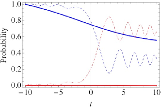
Figure 2: (Color online) (a) Probabilities $|\psi_{i}(t)|^{2}$ for $i=1$ and 2 versus time for $T=40$, $\lambda=0.3$ and $\beta=10$. For comparison, the dashed curves are without decay ($\beta=0$). The inset is a blowup at very small probability. (b) Same as (a), except $T=10$.

Let us now turn to the unexpected result that for large $\beta$, $\Delta P\equiv P(T;\lambda,\beta)-P(T;\lambda,0)>0$ as evident in Figs. 2. We already stressed that this occurs at finite $T$. Moreover, we see from Fig. 2 that $P(T=10)>P(T=40)$. Upon taking the limit $T\to\infty$, we find $\Delta P(T)\to 0$ in accordance with the result in Ref. Akulin_Schleich_92 .

To understand how decay can increase the survival probability $P(T;\lambda,\beta)$, it is instructive to consider the eigenvalues of the Hamiltonian in Eq. (7) as a function of time in a fashion similar to Ref. VZ_11 where the influence of level widths on anti-crossing was discussed. Inspection of the complex eigenvalues yields the following condition for the crossing of the real part of the eigenvalues at $t=0$ VZ_11 (see also Sec. III.2.1),

$$\beta\geq 4\lambda.$$ (25)

This is shown in Fig. 3(a) which plots the real part of the eigenvalues of the Hamiltonian in Eq. (1) versus time and in Fig. 3(b) which shows the imaginary parts for $\lambda=1$. For $\beta>4$, the real parts of the two eigenvalues cross at $t=0$ while the imaginary parts do not. On the other hand, for $\beta<4\lambda$ crossing is avoided. Figure 3(c) and (d) are similar to Fig. 3(a) and (b) but for a smaller decay rate, $\beta=3$, where there is an avoided crossing (as opposed to a crossing). [Similarly, for $\beta>1.2$ the real part of the eigenvalues cross (and the imaginary part of the eigenvalues do not) when $\lambda=0.3$ (as used in Fig. 2). We chose to plot the $\lambda=1$ results in Figs. 3(a) and (b) and and in (c) and (d) because it is easier to see the results when the curves are farther apart.] As the decay rate $\beta$ increases beyond a critical value, the real part of the eigenvalues cross, rather than undergoing an avoided crossing as is the case for $\beta=0$. Hence, the probability at the final time, $P(T;\lambda,\beta)$, increases with increasing $\beta$ for sufficiently large $\beta$.

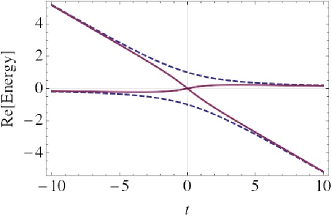
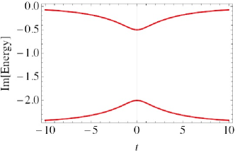
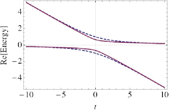
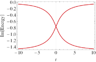
Figure 3: (Color online) (a) Real part of the eigenvalues of the Hamiltonian in Eq. (1) with $\lambda=1$, $\beta=5$ as a function of time (solid red curve). For comparison, the blue dashed curves are the results without decay ($\lambda=1$, $\beta=0$), and have an avoided crossing. (b) Imaginary part of the eigenvalues with $\lambda=1$, $\beta=5$. (c) Real part of the eigenvalues of the Hamiltonian in Eq. (1) with $\lambda=1$ and $\beta=3$ as a function of time (solid red curve). For comparison, the blue dashed curves are for $\lambda=1$ and $\beta=0$, and have a larger splitting. (d) Imaginary part of the eigenvalues with $\lambda=1$ and $\beta=3$.

We now plot the probability $P(T;\lambda,\beta)$ as a function of $\lambda$ and $\beta$. Figure 4(a) shows the results for $T=40$ and Figure 4(b) is for $T=10$. The general trend is that the probabilities decrease significantly with increased $\lambda$ and also increase with increasing $\beta$, but the increase with $\beta$ is much more significant for 4(b). Near $\beta=0$, the first of a series of recurring oscillation peaks that arise from the Stückelberg oscillations evident in Fig. 2 is evident in part (b). This series of peaks stretches on as a function of $\lambda$ at small $\beta$ but is not visible because the figure only goes up to $\lambda=10$. These oscillatory peaks are much smaller in magnitude and are farther appart in $\lambda$ for Fig. 4(a) which is for $T=40$.

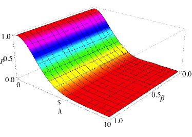
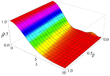
Figure 4: (Color online) (a) Probability $P(T;\lambda,\beta)$ versus $\lambda$ and $\beta$ for $T=40$. (b) Probability $P(T;\lambda,\beta)$ versus $\lambda$ and $\beta$ for $T=10$.

III.2 Results based on the Hamiltonian (17) (saturated energies)

In this section we present results for the saturated of energy levels as specified in the Hamiltonian of Eq. (17). The results are qualitatively similar to those presented previously but the analytic expression (24) enables a simpler and more transparent analysis. Unlike the previous discussion we will focus here only on the long time behavior, beyond which the levels are virtually saturated. First we carry out an elementary analysis of the eigenvalues and find the same condition, $\beta\geq 4\lambda$, for level crossing as in Eq. (25). Then we use (24) to analyze the behavior of $P(T;\lambda,\beta)$. Our analysis includes first a study of the Stückleberg oscillations as a function of the coupling strength $\lambda$ for large $T$, and second, the study of situations where the survival probability increases as $\beta$ approaches (and then surpasses) $4\lambda$ from below.

III.2.1 Analysis of the eigenvalues

In the original LZ problem with linear time dependence of the diagonal elements of the Hamiltonian, without decay, the probability depends crucially on how close the adiabatic energy levels are to one another. Specifically, for small $\lambda$, $P(\infty)$ is high, and for large $\lambda$, $P(\infty)$ decays as $e^{-C/\lambda^{2}}$ where $C$ is a constant. But what happens if there is a decay term, where the Hamiltonian is not hermitian and its eigenvalues are complex? To answer this question it is useful to investigate the instantaneous eigenvalues as a function of time. The eigenvalues of the Hamiltonian $\binom{\tanh t\ \ \ \ \ \ \ \ \ \ \ \ \lambda}{\lambda\ \ \ \ \ -(\tanh t+i\beta}$ are,

$$\varepsilon_{1,2}(t)=\frac{1}{8}\left[-2i\beta\pm\frac{\sqrt{2}}{\cosh t}\sqrt{8i\beta\sinh t-\{16(1-\lambda^{2})+\beta^{2}+[\beta^{2}-16(1+\lambda^{2})]\cosh 2t\}}\right].$$ (26)

Crossing (complex) levels occurs when $\varepsilon_{1}=\varepsilon_{2}$, namely, the expression inside the square root should vanish for some value(s) of $t$. Closer inspection shows that a real solution can occur only for $t=0$, where the expression inside the square root equals $2(16\lambda^{2}-\beta^{2})$. From this simple analysis we can draw the following conclusions [results (1)-(4) pertain to the case $4\lambda\geq\beta$ while result (5) pertains to $4\lambda<\beta$] linear_eig :
(1) The square root at $t=0$ is real, therefore ${\mathrm{Im}}[\varepsilon_{1}(0)$] = ${\mathrm{Im}}[\varepsilon_{2}(0)]=-\beta/4$, i.e., the imaginary parts of the (complex) energies cross at $t=0$.
(2) Im[$\varepsilon_{i}(t)$] is an antisymmetric function of $t$ with respect to the crossing point -$\beta/4$.
(3) Re[$\varepsilon_{i}(t)]\neq 0$ is a symmetric function of $t$, and ${\mathrm{Re}}[\varepsilon_{1}(t)]=-{\mathrm{Re}}[\varepsilon_{2}(t)]>0$. Hence, the real parts of the energies do not cross for $\beta<4\lambda$.
(4) As $\beta\to 4\lambda$ from below, Re[$\varepsilon_{1}(0)]\to 0^{+}$ and Re[$\varepsilon_{1}(0)]\to 0^{-}$. Combined with result (1), the complex energy eigenvalues cross at $t=0$.
Points (1)-(4) are summarized in Figs. 5(a) and (b).
(5) For $4\lambda>\beta$ the real parts of the complex energies cross at $t=0$ but the imaginary parts do not. The probability depends mainly on the behavior of the real parts of the eigenvalues, so that $P(T;\lambda,\beta)$ increases with $\beta$ even in this case. Result (5) is summarized in Figs. 5(c) and (d). Hence, we conclude that for large $\beta$, the probability $P(T;\lambda,\beta)$ is a slowly increasing function of $\beta$. This somewhat counter intuitive result is confirmed by our analytical result (24) for $\psi_{1}(T)$.

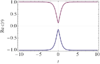
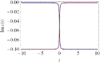
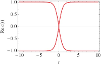
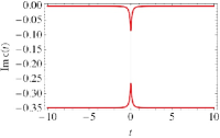
Figure 5: Complex egenenergies of the Hamiltonian $H=\binom{\tanh t\ \ \ \ \ \ \ \ \ \ \ \ \ \lambda}{\lambda\ \ \ \ \ \ -(\tanh t+i\beta}$ as a function of time. (a) ${\mathrm{Re}}[\varepsilon(t)]$, and (b) ${\mathrm{Im}}[\varepsilon(t)]$, with $\lambda=0.15$ and $\beta=0.2$. Since $4\lambda>\beta$, the corresponding level pattern is as discussed in points (1)-(4). (c) ${\mathrm{Re}}[\varepsilon(t)]$, and (d) ${\mathrm{Im}}[\varepsilon(t)]$, with $\lambda=0.15$ and $\beta=0.7$. Since $4\lambda<\beta$, the corresponding level pattern is as discussed in point (5) above.

III.2.2 Stückelberg oscillations with $\lambda$ and the increase of $P(T;\lambda,\beta)$ with $\beta$

In the present section we focus on two aspects of $P(T;\lambda,\beta)$ for fixed and large $T$. First we study Stückelberg oscillations with $\lambda$ for finite decay rate, $\beta>0$, and then we show that $P(T;\lambda,\beta)$ can increase with increasing $\beta$. As will become evident, these two aspects of the LZ dynamics are intimately related.

In Sec. III.1 we encountered Stückelberg oscillations of $|\psi_{1}(t)|^{2}$ with time for $\beta=0$ and fixed $\lambda$. Here we show that there are also Stückelberg oscillations of $P(T;\lambda,\beta)$ with varying $\lambda$ and finite but small $\beta$. We also show that $P(T;\lambda,\beta)$ increases with $\beta$ for sufficiently large $\beta$. Using the analytic expression (14) for the wave function $\psi_{1}(T)$ we compute $P(T;\lambda,\beta)$, and elucidate its dependence on the relevant parameters. The results of this section are illustrated in Fig. 6 which contains a 3D plot of $P(T;\lambda,\beta)$. The main features that can be deduced from this figure are outlined in the caption. In brief, (1) the Stückelberg oscillations are quite sizable at $\beta=0$ (no decay), and are much milder for small $\beta$, and eventually die out at larger $\beta$. This decay of the oscillations can be deduced from the initial Hamiltonian (17); for large $\beta$, the element $H_{22}(t)$ is dominated by its imaginary part. (2) As mentioned in the previous discussion, there are cases where $P(T;\lambda,\beta)$ for fixed $\lambda$ increases with $\beta$. This is especially evident when the probability is examined for $\lambda$ that corresponds to a minimum of a Stückleberg oscillation, (e.g $\lambda\approx 0.5$ in Fig. 6).

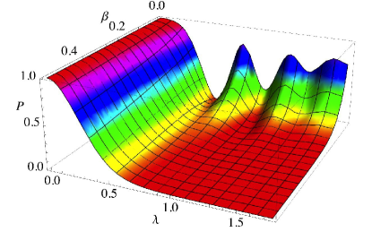
Figure 6: (Color online) The probability $P(T;\lambda,\beta)$ based on Eq. (24) as a function of $\lambda$ and $\beta$ for $T=10$. The main features are the Stückelberg oscillations at $\beta=0$, the decrease of the probability with increasing $\beta$ for small $\lambda$ (e.g., $\lambda=\approx 0.2$), the decay of $P$ with increasing $\beta$ for moderate $\beta$ (e.g., $\beta=0.3$), and the slow increase of $P$ as as a function of $\beta$ near the minimum of the Stückelberg oscillations for small $\lambda$ (i.e., $\lambda\approx 0.5$).

We can further elaborate on this (somewhat counter-intuitive) result with the help of a few two dimensional plots. In Fig. 7(a) the probability $P(T;\lambda,\beta)$ is plotted as a function of $\lambda$ for $\beta=0$ (dashed curve) and for $\beta=0.4$ (solid curve) for $T=6$. For $\beta=0$ the Stükelberg oscillations with $\lambda$ are quite violent, but they are also noticeable for finite decay rate $\beta=0.4$. For small $\lambda$, there are cases where the probability increases with $\beta$, as already noted in connection with Fig. 2. This remarkable observation is further corroborated in Fig. 7(b) which displays the probability $P(T;\lambda,\beta)$ for $T=6$ as function of $\beta$ for fixed $\lambda=0.4$ (dashed curve) and for $\lambda=0.6$ (solid curve).

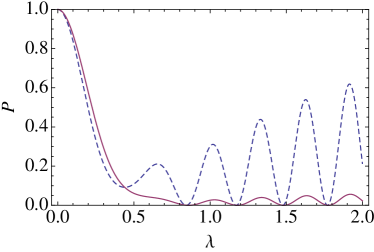
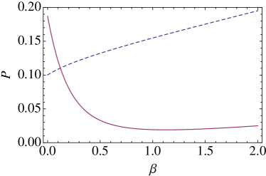
Figure 7: (a) Stückelberg oscillations of $P(T;\lambda,\beta)$ with $\lambda$. The probability $P(T;\lambda,\beta)$ for $T=6$ versus $\lambda$ for $\beta=0$ (dashed curve) and for $\beta=0.4$ (solid curve). (b) The probability $P(T;\lambda,\beta)$ versus $\beta$ for fixed $\lambda=0.4$ (dashed curve) and for $\lambda=0.6$ (solid curve). For $\lambda=0.4$ (dashed curve), $\beta=0$ is a minimum of the first Stückelberg oscillation [see part (a)]; hence, $P(T;\lambda,\beta)$ increases monotonically with increasing $\beta$. For $\lambda=0.6$ (solid curve), $\beta=0$ is close to the maximum of the first Stückelberg oscillation [see part (a)] and $P(T;\lambda,\beta)$ decreases at small $\beta$ and then slowly increases at higher $\beta$.

The probability $P(T;\lambda,\beta)=|\psi_{1}(T)|^{2}$, determined using Eq. (24), is plotted versus $\lambda$ for $\beta=0$ and $\beta=0.2$ in Fig. 8(a). The Stückelberg oscillations for $\beta=0$ (dashed curve) are indeed strong, but for $\beta=0.2$ (solid curve) they are subdued, and the probability is diminished relative to the probability for $\beta=0$. However, compared with the first minimum of $P(T;\lambda,\beta)$ for $\beta=0$ at $\lambda\approx 0.55$, the probability increases with $\beta$. We attribute this surprising result to the fact that level decay induces level crossing. This is especially pronounced when $P(T;\lambda,\beta=0)$ is a minimum point in the pattern of Stückleberg oscillations.

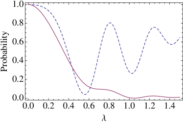
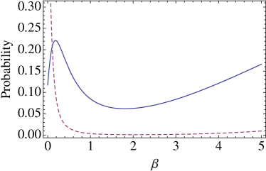
Figure 8: (a) The probability $P(T;\lambda,\beta)$ calculated using Eq. (24) as function of $\lambda$ for $T=10$, and $\beta=0$ (dashed curve) and $\beta=0.2$ (solid curve). Note that between $\lambda=0.45$ and 0.61, the curve with decay is larger than without decay. (b) The probability $P(T;\lambda,\beta)$ based on Eq. (24) as function of $\beta$ for $T=10$, and $\lambda=0.5$ (solid curve) and $\lambda=0.8$ (dashed curve). For $\lambda=0.5$ (solid curve), $\beta=0$ is at a minimum of the first Stückelberg oscillation [see part (a)] and $P(T;\lambda,\beta)$ increases with increasing $\beta$, then decreases and subsequently slowly increases. For $\lambda=0.8$ (dashed curve), $\beta=0$ is close to the maximum of the first Stückelberg oscillation [see part (a)] and $P(T;\lambda,\beta)$ decreases with increasing $\beta$ at small $\beta$, and then slowly increases at higher $\beta$.

Figure 8(b) plots the probability $P(T;\lambda,\beta)$ as function of $\beta$ for $\lambda=0.5$ (solid line) and $\lambda=0.8$ (dashed line). Consider first the solid curve for $\lambda=0.5$, related to the discussion of Fig. 8(a). The curve starts at the first minimum of the Stückelberg oscillations and reaches a local maximum, after which it decays, as expected for a problem with increasing decay rate. However, at higher $\beta$, it approaches and then crosses the curve $\beta=4\lambda$. As discussed in points (4) and (5), the probability increases, which is counter-intuitive. For $\lambda=0.8$ $P(T;\lambda,\beta)$ starts its decay right at the onset as expected, but again, unexpectedly, it starts to increase at higher $\beta$ since $\beta$ approaches and crosses the point $\beta=4\lambda=3.2$. For strong coupling $\lambda$, however, this rise of $P(T;\lambda,\beta)$ is less visible.

IV Numerical Results for the LZ problem with decay of both levels

Systems for which both levels in the LZ dynamics undergo decay to states outside the two-level manifold exist in nuclear and mesoscopic systems VZ_11 . From our study in the previous sections we learned that the dependence of $P(T;\lambda,\beta_{1},\beta_{2})$ on $\beta_{2}$ is sometimes not simple. But its dependence on $\beta_{1}$ is much simpler. Clearly, in the absence of coupling ($\lambda=0$), the probability $P(T;\lambda,\beta_{1},\beta_{2})$ decays exponentially with $\beta_{1}$. As we shall see below, switching on the coupling $\lambda$ does not affect this behavior in any significant way. We start from the symmetric form of the Hamiltonian, corresponding to $Z_{1}(t)=\tfrac{1}{2}(t-i\beta)$ and $Z_{2}(t)=-\tfrac{1}{2}(t+i\beta)$ in Eq. (3). Such a Hamiltonian corresponds to the case of spin $S=1$ states with $M_{S}=1$ and $M_{S}=-1$ in the presence of an external magnetic field along the $z$-axis whose strength is changed linearly in time. Adding decay to both levels yields the Hamiltonian

$${\cal H}(t)=\left(\!\!\begin{array}[]{cc}\tfrac{1}{2}(t-i\beta_{1})&\lambda\\ \lambda&-\tfrac{1}{2}(t+i\beta_{2})\end{array}\!\!\right),$$ (27)

The eigenvalues of this Hamiltonian are

$$\varepsilon_{1,2}(t)=\frac{1}{4}\left[-i(\beta_{1}+\beta_{2})\pm\sqrt{[2t-i(\beta_{1}-\beta_{2})]^{2}+16\lambda^{2}}\right].$$ (28)

The factor $-i(\beta_{1}+\beta_{2})$ appears in both eigenvalues and affects the decay dynamics by introducing exponential decay of the time-dependent wave function Burshtein_88 . When $|\beta_{1}-\beta_{2}|\geq 4\lambda$ the eigenvalues cross. Figure 9 plots the real and imaginary parts of the eigenvalues for $\lambda=1$ for three different cases of decay constant pairs: (1) $\beta_{1}=\beta_{2}=4$, where there is an avoided crossing, (2) the borderline case, $2\beta_{1}=\beta_{2}=8$ so that $|\beta_{1}-\beta_{2}|=4\lambda$, which is the onset of crossing, and (3) $\beta_{1}=4$ and $\beta_{2}=10$. In the examples of the dynamics that follow, the consequences of the avoided crossing or crossing will be very noticeable.

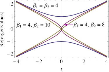
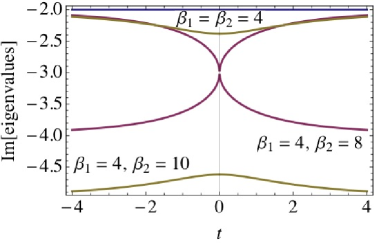
Figure 9: (Color online) For the Hamiltonian in Eq. (27) with $\lambda=1$, (a) ${\mathrm{Re}}[\varepsilon_{1,2}(t)]$ versus time, (b) ${\mathrm{Im}}[\varepsilon_{1,2}(t)]$ versus time.

When $\beta_{1}\neq 0$, it is expected that $P(T;\lambda,\beta_{1},\beta_{2})$ decay exponentially with $\beta_{1}$. More precisely, assume for the moment that there is no level interaction, e.g., if $\lambda=0$, then, $\psi_{1}(t)=e^{i(t^{2}-T^{2})/4}e^{-\beta_{1}(t+T)/2}$. Thus, the survival probability is $P(T;\lambda,\beta_{1},\beta_{2})=|\psi_{1}(T)|^{2}=e^{-\beta_{1}T}$. Switching on the coupling, $\lambda\neq 0$, affects the above result (valid for $\lambda=0$) due to depopulation of level 1. In particular, it leads to the possible increase of $P(T;\lambda,\beta_{1},\beta_{2})$ with $\beta_{2}$, but, as we shall see in Fig. 11, in a much less significant fashion than in the former case where $\beta_{1}=0$. Thus, when $\beta_{1},\beta_{2}\neq 0$ the exponential decay is the dominant feature of the dynamics.

Figure 10(a) shows the probability $P(T;\lambda,\beta_{1},\beta 2)$ for the case where $\beta_{1}=\beta_{2}\equiv\beta$, as a function of $\lambda$ and $\beta$. The probability decays exponentially in both $\lambda$ and $\beta$, but the physics of each decay in each variable is distinct. Decay with $\lambda$, accompanied by Stückelberg oscillations for small $\beta$ which reflects the interference effect in the avoided crossing dynamics, is due to the avoided crossing, whereas the decay with $\beta$ reflects the exponential factor $e^{-\beta T}$ as discussed above. To show this, we multiply the probability by $e^{\beta T}$ and plot $e^{\beta T}\,P(T;\lambda,\beta,\beta)$ as a function of $\lambda$ and $\beta\equiv\beta_{1}=\beta_{2}$ in Fig. 10(b). This kind of plot was first suggested in Ref. Burshtein_88 . The figure clearly shows that $e^{\beta T}\,P(T;\lambda,\beta,\beta)$ is independent of $\beta$. Of course, for the case $\beta_{1}=\beta_{2}=\beta$, this result is expected because then the decay term enters as $-i(\beta/2){\bf I}_{2\times 2}$, therefore $\psi_{1}(T,\beta)=\exp^{-(\beta/2)T}\psi_{1}(T,0)$.

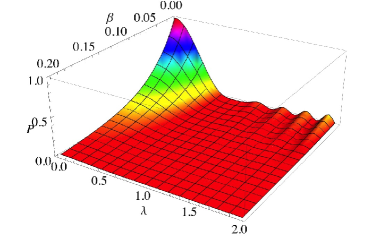
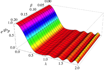
Figure 10: (Color online) (a) The probability $P(T;\lambda,\beta_{1},\beta_{2})$, calculated using the Hamiltonian Eq. (27), as a function of $\lambda$ and $\beta\equiv\beta_{1}=\beta_{2}$ for $T=10$. (b) $e^{\beta T}\,P(T;\lambda,\beta,\beta)$ calculated using the Hamiltonian Eq. (27) as a function of $\lambda$ and $\beta\equiv\beta_{1}=\beta_{2}$ for $T=10$.

Finally we address the question of how $\beta_{1}\neq 0$ affects the observation that $P(T;\lambda,\beta_{1}=0,\beta_{2})$ might increase with $\beta_{2}$. Figure 11 shows the probability $P(T;\lambda,\beta_{1},\beta_{2})$ as function of $\beta_{2}$ for fixed $\lambda=0.4$ for two values of $\beta_{1}$, $\beta_{1}=0$ (dashed curve) and $\beta_{1}=0.1$ (solid curve). The effect of level crossing is reflected by the slow increase of $P(T;\lambda,\beta_{1},\beta_{2})$ with $\beta_{2}$ is clearly seen for $\beta_{1}=0$ while it is hardly visible for $\beta_{1}=1$.

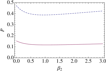
Figure 11: (Color online) The probability $P(T;\lambda,\beta_{1},\beta_{2})$ for $T=6$ as a function of $\beta_{2}$ for fixed $\lambda=0.4$ and for two values of $\beta_{1}$, $\beta_{1}=0$ (dashed curve) and $\beta_{1}=0.1$ (solid curve). The effect of level crossing reflected by the slow increase of $P(T;\lambda,\beta_{1},\beta_{2})$ with $\beta_{2}$ is clearly seen for $\beta_{1}=0$ while it is hardly visible even at small $\beta_{1}$, e.g., $\beta_{1}=0.1$.

V Landau–Zener Problem with dephasing

Dephasing is one of the causes of decoherence of a quantum system, and is due to the interaction of the system with its environment (see Sec. I). Dephasing results in the scrambling of the phases of the amplitudes appearing in the system wave function. In the context of magnetic resonance phenomena, decay and dephasing are often called $T_{1}$ and $T_{2}$ processes respectively. In this section we describe an approach for treating the LZ problem with dephasing which uses a stochastic Schrödinger–Langevin differential equation approach. We also relate this to the master equation (density matrix) approach, at least for Gaussian white noise (we also consider Gaussian colored noise). For Gaussian white noise, the stochastic Schrödinger–Langevin approach is equivalent to a master equation approach with Lindblad terms vanKampenBook . We shall calculate the average over stochastic realizations of the LZ survival probability, $\overline{P(t)}$, the standard deviation of the probability, $\Delta P(t)=\sqrt{\overline{P(t)^{2}}-(\overline{P(t)})^{2}}$, and the distribution ${\cal D}[P(T)]$ of the probability $P(T)$ at the final time, and analyze the dependence on the LZ parameters and the dephasing strength.

V.1 Analogy with spin 1/2 particle in a stochastic magnetic field

It is useful to use the analogy of a spin 1/2 particle under the influence of a time-dependent stochastic magnetic field to exemplify the role of dephasing in the LZ problem. Following Refs. STB_2013 ; Rammer ; Efrat2 , the bare LZ Hamiltonian ${\cal H}_{0}$ is a $2$$\times$$2$ matrix that is formally written as ${\cal H}_{0}={\bm{\sigma}}\cdot{\bf B}_{0}(t)$, where ${\bf B}_{0}$ is the intrinsic “magnetic field”. Interaction with the environment is modeled using a Hamiltonian ${\cal H}_{1}={\bm{\sigma}}\cdot{\bf b}(t)$ where ${\bf b}(t)$ is the external stochastic “magnetic field”. For $T_{2}$ dephasing processes, we take ${\bf b}(t)=\xi(t)\hat{\bf z}$ where $\xi(t)$ is white noise. The average over the noise fluctuations and the second moment are given by

$$\overline{\xi(t)}=0,\quad\overline{\xi(t)\xi(t^{\prime})}=\xi_{0}^{2}\,\delta(t-t^{\prime}),$$ (29)

where $\xi_{0}$ is the volatility (the stochastic field strength) which is inversely proportional to the dephasing time $\tau_{\phi}$, $\overline{(\ldots)}$ denotes the stochastic average, and $\delta(\bullet)$ is the Dirac $\delta$ function. The white noise, $\xi(t)$, can be written as the time derivative of the Wiener process, $\xi(t)=dw(t)/dt$, or more formally, the Wiener process $w(t)$ is the integral of the white noise.

As before, the initial state of the spin at $t=-T$ is $\psi_{1}(-T)=|\!\uparrow\rangle=\binom{1}{0}$, and we seek the probability $P(T)$ that it will stay at a state $|\!\uparrow\rangle$ at $t=T$. Our approach is to numerically solve the time-dependent Schrödinger with a stochastic term proportional to $w(t)$. Since $w(t)$ is a stochastic process, $P(t)$ is also, and it has a distribution ${\cal D}[P(t)]$. Usually, interest is focused on the averaged probability, $\overline{P}=\int_{0}^{1}{\cal D}(P)dP$ at any given time, and in particular, the final time. More information, however, is encoded in the distribution ${\cal D}(P)$ of the probability, and this is less well-studied.

V.2 Stochastic time-dependent Schrödingier equation

There are several ways of modeling stochastic processes, including a master equation method master_eq , a Monte Carlo wave-function method Molmer_93 , or a stochastic differential equations method. Here, we model dephasing using stochastic differential equations vanKampenBook ; Kloeden ; Kloeden_03 ; Gardiner . We briefly elaborate on the time-dependent Schrödingier equation for the LZ problem with a stochastic term that models dephasing processes, and its solution. For the Hamiltonian in Eq. (7), the stochastic equations can be written as

$${\dot{\psi}}_{1}(t)=-i\lambda\psi_{2}(t)+\xi_{0}\xi(t)\psi_{1}(t)-\frac{\xi_{0}^{2}}{2}\psi_{1}(t),$$ (30a)

$${\dot{\psi}}_{2}(t)=-i[\lambda\psi_{1}(t)+z(t)\psi_{2}(t)]-\xi_{0}\xi(t)\psi_{2}(t)-\frac{\xi_{0}^{2}}{2}\psi_{2}(t),$$ (30b)

where $z(t)=-t/2$ and $\xi_{0}$ is a dimensionless volatility which is inversely proportional to the dimensionless dephasing time $\tau_{\phi}$. These equations can be rewritten in the notation of stochastic differential equations Kloeden ; Kloeden_03 ; Gardiner as

$$d\psi_{1}(t)=-i\lambda\psi_{2}(t)dt-\frac{\xi_{0}^{2}}{2}\psi_{1}(t)dt+\psi_{1}(t)\,dw,$$ (31a)

$$d\psi_{2}(t)=-i[\lambda\psi_{1}(t)dt+z(t)\psi_{2}(t)dt]-\frac{\xi_{0}^{2}}{2}\psi_{2}(t)dt-\psi_{2}(t)\,dw,$$ (31b)

where $w(t)$ is the Wiener process, i.e., $\xi(t)=dw(t)/dt$. The $\xi_{0}^{2}$ terms in these equations insure unitarity vanKampenBook . For any fixed realization of the stochastic process, the equations are solved to yield the two component spinor $\binom{\psi_{1}(t)}{\psi_{2}(t)}$ and the survival probability at time $t$ is $P(t)=|\psi_{1}(t)|^{2}$. The distinction as compared with the deterministic case $\xi_{0}=0$ is that now $P(t)$ is a random function with distribution ${\cal D}[P(t)]$ (see Sec. V.3).

Equations (30) [or (31)] are a special case of the Schrödinger–Langevin equation vanKampenBook ,

$${\dot{\psi}}=-i{\cal H}\psi+\xi_{0}\xi(t){\cal V}\psi-\frac{\xi_{0}^{2}}{2}{\cal V}^{{\dagger}}{\cal V}\psi.$$ (32)

In our case, ${\cal V}=\sigma_{z}$, and $\psi$ is a two component spinor. Equation (32) can be generalized to include sets of operators ${\cal V}_{j}$, stochastic processes $w_{j}(t)$, and volatilities $w_{0,j}$, to obtain the general Schrödinger–Langevin equation,

$${\dot{\psi}}=-i{\cal H}\psi+\sum_{j}\left(\xi_{0,j}\xi_{j}(t){\cal V}_{j}\psi-\frac{\xi_{0,j}^{2}}{2}{\cal V}^{{\dagger}}_{j}{\cal V}_{j}\psi\right).$$ (33)

The average over stochasticity obtained using Eq. (33) will be equal the result obtained using a Markovian quantum master equation for the density matrix $\rho(t)$ with Lindblad operators ${\cal V}_{j}$ vanKampenBook ; master_eq ,

$${\dot{\rho}}=-i[{\cal H},\rho(t)]+\frac{1}{2}\sum_{j}w_{0,j}^{2}\left(2{\cal V}_{j}\rho(t){\cal V}^{{\dagger}}_{j}-\rho(t){\cal V}^{{\dagger}}_{j}{\cal V}_{j}-{\cal V}^{{\dagger}}_{j}{\cal V}_{j}\rho(t)\right).$$ (34)

A numerical demonstration of the equivalence is presented in Ref. Band_RWA . However, the master equation will not yield the variance or the statistics or the distribution, quantities that can be obtained from the stochastic Schrödinger–Langevin equation approach.

There are many other kinds of stochastic processes. For example, a well-known stochastic process is Brownian motion, also known as Gaussian colored noise and the Ornstein–Uhlenbeck process OU_30 . For this type of stochastic dephasing process process, the stochastic differential equations are,

$$d\psi_{1}(t)=-i\lambda\psi_{2}(t)dt+\psi_{1}(t)\,{\cal O}(t),$$ (35a)

$$d\psi_{2}(t)=-i[\lambda\psi_{1}(t)dt+z(t)\psi_{2}(t)dt]-\psi_{2}(t)\,{\cal O}(t),$$ (35b)

$$d{\cal O}(t)=\vartheta[\mu-{\cal O}(t)]\psi_{2}(t)dt+\sigma dW(t),$$ (35c)

where the mean autocorrelation function of the Ornstein–Uhlenbeck process are

$$\overline{{\cal O}(t)}={\cal O}_{0}\,e^{-\vartheta t}+\mu(1-e^{-\vartheta t}),\quad\overline{{\cal O}(t)\,{\cal O}(t^{\prime})}=\frac{\sigma^{2}}{2\vartheta}e^{-\vartheta(t+t^{\prime})}[e^{\vartheta\,{\mathrm{min}}(t,t^{\prime})}-1],$$ (36)

$\vartheta$ is the mean reversion rate of the Ornstein–Uhlenbeck process ${\cal O}(t)$, $\sigma$ is the volatility, and $\mu$ is the mean, which we take to vanish, $\mu=0$; we also take ${\cal O}_{0}=0$. This process yields a non-Markovian master equation for the density matrix of the system.

V.3 The Landau–Zener problem with dephasing: Numerical results

Figure 12 shows the results of calculations implemented with the Mathematica 9.0 built-in command ItoProcess ItoProcess carried out using Eqs. (31). We took $\lambda=0.3$ and $T=10$, so we can directly compare with the deterministic results (without noise, i.e., with $\xi_{0}=0$) shown as the dashed curves in Fig. 2(b). We had to shift the time so that we start the process at $t=0$, rather than $t=-T$, and end it at $t=2T$, in order to get ItoProcess to work. Figure 12(a) plots fifty stochastic realizations of the survival probability $P(t;\lambda)=\psi_{1}^{*}(t)\psi_{1}(t)$ versus time for relatively weak disorder ($\xi_{0}=0.2$) and Fig. 12(b) plots the averaged probability $\overline{P(t)}=\overline{\psi_{1}^{*}(t)\psi_{1}(t)}$ (red curve), and mean values plus and minus the standard deviations (blue curves) versus time for 300 realizations. Unitarity, i.e., $\langle\psi(t)|\psi(t)\rangle=1$ is preserved for each path (realization), as insured by the $\xi_{0}^{2}$ terms in Eqs. (31). Clearly, the mean $\overline{P(t)}$ is very close to the probability without noise shown in Fig. 2(b) [whose analytic form is given in terms of Eqs. (11a) and (11b)], despite the fact that the standard deviation at large times is as large as the mean (the dephasing is not small in this sense). The evolution of the standard deviation grows with time but saturates at large times.

Let us now consider the stochastic dynamics in the strong system-environment coupling regime. Figure 13 shows the results for $\xi_{0}=1.0$ and $\lambda=0.3$. The mean probability, $\overline{P(t)}$, is significantly higher and very different in shape than the probability shown in Fig. 2(b). This is a general trend of strong dephasing for arbitrary $\lambda$ (see below). At the final time we find, $\overline{P(\xi_{0}=1.0)}-P(\xi_{0}=0)\approx 0.62-0.35$ with a standard deviation of about 0.3. Furthermore, for strong system-environment coupling, the dephasing almost completely attenuates the interference, which is so significant for the transition with $\lambda=0.3$ and no dephasing.

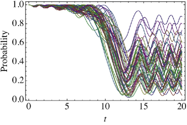
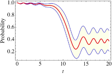
Figure 12: (Color online) Landau–Zener problem with dephasing. (a) The probability $P(t;\lambda)=\psi_{1}^{*}(t)\psi_{1}(t)$ versus time for $\lambda=0.3$ and $T=10$ (i.e., the total elapsed time is $2T=20$) for fifty paths (stochastic realizations) with dimensionless volatility $\xi_{0}=0.2$ [see Eq. (29)]. (b) Average $\overline{P_{1}(t;\lambda)}=\overline{\psi_{1}^{*}(t)\psi_{1}(t)}$ with 300 stochastic realizations and the average plus and minus standard deviation of the probability versus time.

Figure 13: (Color online) Same as Fig. 12, except with $\xi_{0}=1.0$. Average $\overline{P_{1}(t;\lambda)}$ and standard deviation over the 300 realizations. Compared with Fig. 2(b) (dashed blue curve), where $P(T=10,\xi_{0}=0)=0.3$, the noise-averaged probability for high dephasing rate is much higher, $\overline{P}(t_{f};\xi_{0}=1)=0.6$ where $t_{f}=2T=20$.

It is instructive to explicitly consider the distributions ${\cal D}[P(T)]$ for weak and strong couplings. Figure 14 shows the histogram of the probabilities at the final time, $P(T)=\psi_{1}^{*}(T)\psi_{1}(T)$ for $\lambda=0.3$, $T=10$ for $\xi_{0}=0.2$ and $\xi_{0}=1.0$. One clearly sees that the two distributions are quite different. For weak coupling, the distribution is peaked around the mean value which is the same as for $\xi_{0}=0$, but for strong coupling, the peak of the distribution is shifted to higher probabilities (near $P=1$) and the width of the distribution is much broader (standard deviation about 0.3). This result is in line with the findings in Ref. Efrat2 . Similarly, for $\lambda=0.2$; at the final time we find, $\overline{P(\xi_{0}=1.0)}-P(\xi_{0}=0)\approx 0.73-0.635$, so the average probability is shifted to a higher value due to strong dephasing, and the standard deviation is about 0.2 [see results at the final time in Fig. 15(b)]. Moreover, the distribution is significantly skewed to higher probabilities (see below). Figure 15(a) shows the probabilities $P_{1}(t)$ and $P_{2}(t)$ versus time without dephasing for $\lambda=0.2$, Fig. 15(b) plots the mean and variance of the LZ probability as a function of time, and Fig. 15(c) shows the histogram of the probabilities at the final time $P(T)$. The shifted average probability and the skewed probability distribution ${\cal D}[P(T)]$ show that dephasing increases the survival probability. This seems to be a general trend under relatively strong dephasing conditions (as opposed to relatively weak dephasing where, even though the standard deviation of the survival probability can be large, the average probability is largely unaffected) comment . We note that for extremely large $\xi_{0}$, it becomes difficult to control the numerics so as to maintain unitarity.

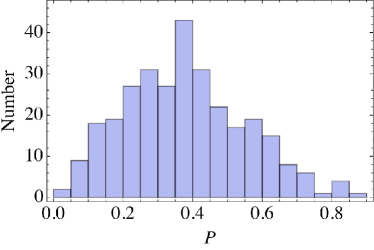
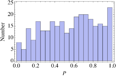
Figure 14: (Color online) Histograms of $P(T;\lambda)=\psi_{1}^{*}(T)\psi_{1}(T)$ with dephasing. We used $\lambda=0.3$, $T=10$ (the total elapsed time is $2T=20$) with 300 paths (stochastic realizations). (a) $\xi_{0}=0.2$ and (b) $\xi_{0}=1$.

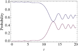
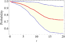
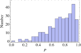
Figure 15: (Color online) (a) Probabilities $P(t;\lambda)\equiv P_{1}(t;\lambda)=\psi_{1}^{*}(t)\psi_{1}(t)$ (blue upper curve) and $P_{2}(t;\lambda)=\psi_{2}^{*}(t)\psi_{2}(t)$ (red lower curve) versus time for $\lambda=0.2$ and $T=10$ (the total elapsed time is $2T=20$) calculated without dephasing. (b) Mean and standard deviation of the LZ probability $P(t;\lambda)$ calculated with dephasing using 300 paths (stochastic realizations) and $\xi_{0}=1$. (c) Histogram of $P(t_{f};\lambda)$, where $t_{f}=2T=20$, with 300 paths and strong dephasing, $\xi_{0}=1$.

We present results obtained with the same parameters used to obtain Fig. 15, except that now we take the stochastic process to be the Ornstein–Uhlenbeck process (Brownian motion). We use Eqs. (35) with $\mu=0$, $\vartheta=1$, $\sigma=1$ and ${\cal O}_{0}=0$. The dynamics will now not be Markovian, as opposed to the dyanmics using white Gaussian noise. Figure 16(a) shows 100 stochastic realizations of $P(t;\lambda)$, Fig. 16(b) shows the mean and variance of the probability $P(t;\lambda)$ as a function of time computed with 400 realizations, and 16(b) shows the histogram of the probabilities at the final time, $P(T)$, with 400 realizations. We see that the mean of the probability goes at the final time to about 0.55, even for $T=10$, whereas the white noise mean is about 0.73 (recall that without dephasing, the final probability is 0.635 for these conditions).

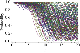
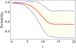
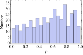
Figure 16: (Color online) (a) 100 stochastic realizations of the probability $P(t;\lambda)\equiv P_{1}(t;\lambda)=\psi_{1}^{*}(t)\psi_{1}(t)$ for $\lambda=0.2$ and $T=10$ (the total elapsed time is $2T=20$) . (b) mean and standard deviation of $P(t;\lambda)$ with 400 paths (stochastic realizations) for $\sigma=\vartheta=1$, $\mu=0$ and ${\cal O}_{0}=0$. (c) Histogram of the probability $P(T;\lambda)$ with 400 paths.

Finally, we briefly explore the LZ problem with the combined effects of one-level decay and dephasing. The object of study is the mean LZ probability $\overline{P(T;\lambda,\beta,\xi_{0})}$ at long but finite time $T$. The questions to be asked are: (1) For fixed decay strength $\beta>0$, how does the presence of dephasing $\xi_{0}>0$ affect $\overline{P(T;\lambda,\beta,\xi_{0})}$ as compared with the LZ probability $P(T;\lambda,\beta,0)$ (no depjasing)? (2) For fixed dephasing strength $\xi_{0}>0$, how does the presence of decay $\xi_{0}>0$ affect the behavior of $\overline{P(T;\lambda,\beta,\xi_{0})}$ as function of $\beta$? In other words, is the counterintuitive observation, analyzed previously in the absence of dephasing, (that there are situations where $P$ increases with $\beta$), survive also in the presence of dephasing? To answer these questions we present the results of calculations based on the linear model, with decay and dephasing, i.e., Eqs. (30a) and (30b) albeit with $z(t)=-\tfrac{1}{2}(t+i\beta)$, in Fig. 17. This figure should be compared with Fig. 12 (which displays the results of calculations with dephasing in the absence of decay), and Fig. 2 (which displays the results of calculations with decay in the absence of dephasing). The main results of this analysis can be stated briefly as follows: (i) Comparing Figs. 17(b) and 2(b) shows that for large enough $\beta\approx T$, the effect of dephasing on $\overline{P(t;\lambda,\beta,\xi_{0})}$ is small. (ii) Comparing the parts of Figs. 17 with one another and with Fig. 12 shows that: (iia) For small $\beta$ the mean probability slightly decreases with increasing decay, but for large $\beta$ the mean probability increases with increasing $\beta$. In other words, the answer to question (2) posed above is affirmative. (iib) For large decay rate $\beta\geq T$ the variance of the survival probability shrinks.

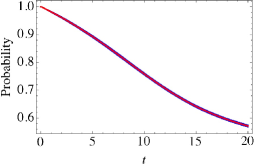
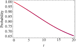
Figure 17: (Color online) Mean and standard deviation of the probability $P(t;\lambda,\beta,\xi_{0})$ for the LZ problem with one-level decay of strength $\beta$, dephasing with sterngth $\xi_{0}=0.2$, $\lambda=0.3$, and $T=10$. To be compared with Figs. 2(b) (decay without dephasing) and 12 (dephasing without decay). (a) $\beta=1$ and $\overline{P(T;\lambda,\beta,\xi_{0})}\approx 0.3<\overline{P(T;\lambda,0,\xi_{0})}\approx 0.4$ (see Fig. 12). (b) $\beta=10$ and $\overline{P(T;\lambda,\beta,\xi_{0})}\approx 0.58\approx P(T;\lambda,\beta,0)$ [see Fig. 2(b)]. (c) $\beta=15$ and $\overline{P(T;\lambda,15,\xi_{0})}\approx 0.65>\overline{P(T;\lambda,10,\xi_{0})}$. The variance in (b) and (c) is very small (barely visible).

VI Summary and conclusions

We studied two aspects of the classical Landau–Zener problem. First, the Landau–Zener problem with decay was analyzed using a combination of analytic and numeric solutions of the time-dependent Schrödinger equation. The time dependence of the energy levels was taken to be either linear $\varepsilon_{1,2}(t)=\pm\alpha t$ or of the form $\varepsilon_{1,2}(t)=\varepsilon\tanh(t/{\cal T})$. In the first case the energies are not bounded as $|t|\to\infty$. In the long time limit, the probability $P(\infty)$ is independent of decay rate for the linear Landau–Zener case. This is an artifact of the unbounded form of the time-dependent energies appearing in the diagonal elements of the Landau–Zener Hamiltonian. When the energy levels are bounded as function of time between the initial and finite times, the probability does depend on decay rate. Surprisingly, the survival probability of state $\psi_{1}(t)$ increases with increasing decay rate $\beta_{2}$. This is due to level crossing (rather than an avoided crossing) that occurs for sufficiently large $\beta_{2}$ ($\beta_{2}>4\lambda$). These results are valid both for the linear Landau–Zener problem and for the smoothly saturated energies of the form $\varepsilon\tanh(t/{\cal T})$. In the latter case, the analytic solution for the wave function at large $T$ yields a particularly simple analytic expression for the probability.

Let us compare our approach with that of Ref. Schilling_06 , which is closely related to our study of Landau–Zener with decay. It studied the Landau–Zener problem with decay without specifically specifying the precise time dependence of the two energy levels. Berry’s approach with a superadiabatic basis Berry_90 is used to obtain the survival probability $P$ in the slow-sweep limit (small $\alpha$). The main result obtained was that $P$ is composed of two factors, a geometrical and dynamical one, and these factors are analyzed. When applied to the model of Ref. Akulin_Schleich_92 , the independence of $P$ on the decay rate is recovered. Critical damping of Stückelberg oscillations is predicted and analyzed in the region of very small probability, $P<10^{-5}$. Our approach, on the other hand, deals with specific forms of the time dependence of the energy levels and leads to analytic solutions of the pertinent second order differential equations. This enabled us to carry out a systematic analysis of the dependence of $P$ on decay parameters for arbitrary values of decay rate and channel coupling. The independence of $P$ on the decay rate for the linear case is simply explained in terms of the analytic solution, as is the dependence of $P$ on the decay rate for the saturated energy case. Our results are valid for arbitrary sweep rate and interaction strength, as well as on the decay rates $\beta_{1}$ and $\beta_{2}$.

Second, we studied a few aspects of the Landau–Zener problem with dephasing. For an example of such dephasing processes, consider the population transfer within the triplet ground state manifold of diamond NV^- centers Jarmola_12 ; Doherty_13 . In diamond NV centers, the $m_{s}=0$ level is lower in energy than the $m_{s}=\pm 1$ levels due to crystal field effects. Suppose one is interested in moving population from $m_{s}=0$ to $m_{s}=-1$ by slowly sweeping (chirping through resonance) the frequency of a radio-frequency field that is nearly in resonance with the $m_{s}=0\to-1$ transition. The $m_{s}=-1$ state decays to $m_{s}=0$ (longitudinal and transverse decay processes can both take place), and therefore the decay is within the three-level manifold. Generalizing to a stochastic differential Schrödinger–Langevin equation approach enables the treatment of such cases. In Sec. V we carried out this approach for $T_{2}$ dephasing during the Landau–Zener dynamics with both white-noise and Ornstein–Uhlenbeck-noise (a similar procedure can be used to model $T_{1}$ processes if the coupling operator is taken to be ${\cal V}=\sigma_{x}$ rather than $\sigma_{z}$). For Gaussian white noise, his method is equivalent to using a density matrix approach with Lindblad operators vanKampenBook , but produces non-Markovian dynamics for other kinds of noise. References Rammer and Efrat2 showed that for Landau–Zener transitions with dephasing driven by white noise, the underlying physics depends on whether the dephasing time is long (weak dephasing) or short (weak dephasing). The Schrödinger–Langevin equation approach enabled us to compute the survival probability both in the weak and strong dephasing regimes. We calculated the distribution of the survival probability and pointed out its distinct behaviour in the long and short dephasing time regimes, and we showed that Ornstein–Uhlenbeck noise gives somewhat different behavior than Gaussian white noise.

We also analyzed the combined effects of one-level decay and dephasing on the averaged LZ survival probability. We found that the counterintuitive result, that there are situations where the LZ probability increases with decay rate, survives also in the presence of dephasing.

Acknowledgement. This work was supported in part by grants from the Israel Science Foundation (Grant Nos. 400/2012 and 295/2011). We are grateful to Professor Dmitry Budker for stimulating our interest in this problem and for valuable discussions throughout the course of this work. Discussions with Efrat Shimshoni and Robert Shekhter are highly appreciated.

References

- (1) L. Landau, “On the theory of transfer of energy at collisions I”, Phys. Z. Sowjetunion 2, 46 (1932).
- (2) C. Zener, “Non-Adiabatic crossings of energy levels”, Proc. R. Soc. London, Ser. A137, 696 (1932).
- (3) E. C. G. Stückelberg, “Theorie der unelastischen Stösse zwischen Atomen”, Helvetica Physica Acta 5, 369 (1932).
- (4) E. Majorana (1932), “Atomi orientati in campo magnetico variabile”, Nuovo Cimento 9, 43 (1932).
- (5) A. I. Burshtein and A. V. Storozhev, “Transition width between two metastable states”, Chem. Phys. 119, 1 (1988).
- (6) L. Marcassa, V. Bagnato, Y. Wang, C. Tsao, J. Weiner, O. Dulieu, Y. B. Band, P. S. Julienne, “Collisional Loss Rate in a Magneto-Optical Trap for Sodium Atoms: Light Intensity Dependence”, Phys. Rev. A47, R4563 (1993).
- (7) Y. B. Band, I. Tuvi, K.-A. Suominen, K. Burnett, and P. S. Julienne, “Loss from magneto-optical traps in strong laser fields”, Phys. Rev. A50, R2826 (1994).
- (8) V. Bagnato, L. Marcassa, Y. Wang, and J. Weiner, P. S. Julienne, and Y. B. Band, “Ultracold Photo-associative Ionization Collisions in a Magneto-optical Trap: Optical Field Intensity Dependence in a Radiatively Dissapative Environment”, Phys. Rev. A48, R2523 (1993).
- (9) C. J. Hardy, W. A. Edelstein, and D. Vatis, “Efficient Adiabatic Fast Passagefor NMR Population Inversion in the Presence of Radiofrequency Field Inhomogeneity and Frequency Offsets”, J. Magnetic Resonance 66, 470 (1986).
- (10) V. M. Akulin and W. P. Schleich, “Landau–Zener transition to a decaying level”, Phys. Rev. A46, 4110 (1992).
- (11) In Ref. Akulin_Schleich_92 , the solution of the second order differential equation (9a) is expressed in terms of a single transcendental Hermite function, and not as a combination of two independent transcendental functions, as in Eq. (12). The procedure for satisfying the two required initial conditions [the analog of Eq. (13)] is therefore not fully specified.
- (12) G. Dridi, S. Guerin, H. R. Jauslin, D. Viennot, and G. Jolicard, “Adiabatic approximation for quantum dissipative systems: Formulation, topology, and superadiabatic tracking”, Phy. Rev. A 82, 022109 (2010).
- (13) G. Dridi and S. Guerin, “Adiabatic passage for a lossy two-level quantum system by a complex time method”, Journal of Physics A–Mathematical and Theoretical 45, 35 (2012).
- (14) M. Scala, B. Militello, A. Messina, and N. V. Vitanov, “Microscopic description of dissipative dynamics of a level-crossing transition”, Phy. Rev. A84, 023416 (2011).
- (15) R. Uzdin and N. Moiseyev, “Rapid azimuthal rotation in the Hermitian and non-Hermitian Landau–Zener problem”, Journal of Physics A–Mathematical and Theoretical 45, 444033 (2012).
- (16) V. V. Kocharovsky, E. A. Derishev, S. A. Litvak, I. A. Shereshevsky, and S. Tasaki, “Nonstationary dressed states and effects of decay in nonadiabatic crossing of decaying levels”, Computers and Mathematics with Applications 34, 727 (1997).
- (17) V. V. Kocharovsky and S. Tasaki, “ crossing of decaying levels”, in Advances in Chemical Physics, Vol. 99: Resonances, Instability, and Irreversibility, (John Wiley and Sons, New York, 1997), Vol. 99, pp. 333-368.
- (18) K.-A. Suominen, Y. B. Band, I. Tuvi, K. Burnett, and P. S. Julienne, “Quantum and Semiclassical Calculations of Cold Atom Collisions in Light Fields”, Phys. Rev. A57, 3724 (1998).
- (19) N. V. Vitanov and S. Stenholm, “Pulsed excitation of a transition to a decaying level”, Phy. Rev. A 55, 2982 (1997); N. V. Vitanov and S. Stenholm, “Population transfer via a decaying state”, Phy. Rev. A56, 1463 (1997).
- (20) C. A. Moyer, “Quantum transitions at a level crossing of decaying states”, Phy. Rev. A64, 14 (2001).
- (21) V. A. Benderskii, E. V. Vetoshkin and E. I. Kats, “Semiclassical quantization of bound and quasistationary states beyond the adiabatic approximation”, Phy. Rev. A69, 20 (2004).
- (22) E. M. Graefe and H. J. Korsch, “Crossing scenario for a nonlinear non-Hermitian two-level system”, Czechoslovak Journal of Physics 56, 1007 (2006).
- (23) R. Schilling, M. Vogelsberger and D. A. Garanin, “Nonadiabatic transitions for a decaying two-level system: geometrical and dynamical contributions”, J. Physics A–Mathematical and General 39, 13727 (2006).
- (24) B. W. Shore and N. V. Vitanov, “Overdamping of coherently driven quantum systems”, Contemporary Physics 47, 341 (2006).
- (25) B. D. Fainberg, M. Jouravlev and A. Nitzan, “Light-induced current in molecular tunneling junctions excited with intense shaped pulses”, Phy. Rev. B76, 12 (2007).
- (26) H. M. Castro-Beltran, E. R. Marquina-Cruz, G. Arroyo-Correa, and A. Denisov, “Nonstationary dissipative dynamics of a single qubit”, Laser Physics 18, 149-156 (2008).
- (27) Y. Gefen, E. Ben-Jacob and A.O. Caldeira “Zener Transitions in Dissipative Driven Systems”, Phys. Rev. B 36, 2770 (1987).
- (28) P. Ao and J. Rammer, “Influence of Dissipation on the Landau-Zener Transition”, Phys. Rev. Lett. 62, 3004 (1989); “ Quantum dynamics of a two-state system in a dissipative environment”, Phys. Rev. B43, 5397 (1991).
- (29) K. Saito, M. Wubs, S. Kohler, Y. Kayanuma, and P. Hänggi, “Dissipative Landau-Zener transitions of a qubit: Bath-specific and universal behavior”, Phys. Rev. B 75, 214308 (2007).
- (30) E. Shimshoni and Y. Gefen, “Onset of dissipation in Zener dynamics: Relaxation versus dephasing”, Ann. Phys. (NY) 210, 16 (1991).
- (31) E. Shimshoni and A. Stern, “Dephasing of interference in Landau-Zener transitions”, Phys. Rev. B47, 9523 (1993).
- (32) V. L. Pokrovsky and D. Sun, “Fast quantum noise in the Landau-Zener transition”, Phys. Rev. B76, 024310 (2007).
- (33) J. E. Avron, M. Fraas, G. M. Graf and P. Grech, “Landau-Zener Tunneling for Dephasing Lindblad Evolutions”, Commun. Math. Phys. 305, 633 (2011).
- (34) I. L. Aleiner, B. L. Altshuler, and Y. M. Galperin “Experimental tests for the relevance of two-level systems for electron dephasing”, Phys. Rev. B63, 201401(R) (2001).
- (35) D. E. Chang, Jun Ye, and M. D. Lukin, “Controlling dipole-dipole frequency shifts in a lattice-based optical atomic clock”, Phys. Rev. A69, 023810 (2004).
- (36) A. Steane, “Quantum Computing”, Rep. Prog. Phys. 61, 117 (1998); J. I. Cirac, P. Zoller, “New frontiers in quantum information with atoms and ions”, Physics Today 57, 38, March 2004.
- (37) F. Dolde, H. Fedder, M.W. Doherty, T. Nöbauer, F. Rempp, G. Balasubramanian, T. Wolf, F. Reinhard, L. C. L. Hollenberg, F. Jelezko, and J. Wrachtrup, “Electric-field sensing using single diamond spins”, Nat. Phys. 7, 459 (2011); V. M. Acosta, K. Jensen, C. Santori D. Budker and R. G. Beausoleil, “Electromagnetically Induced Transparency in a Diamond Spin Ensemble Enables All-Optical Electromagnetic Field Sensing”, Phys. Rev. Lett. 110, 213605 (2013); J. Zhou, P. Huang, Q. Zhang, Z. Wang, T. Tan, X. Xu, F. Shi, X. Rong, S. Ashhab, and J. Du, “Observation of Time-domain Rabi Oscillations in the Landau–Zener Regime with a Single Electronic Spin”, arXiv:1305.0157.
- (38) N. G. Van Kampen, Stochastic Processes in Physics and Chemistry, (Elsevier, Amsterdam, 1997). See particularly Sec. 7.5 on the Schrodinger-Langevin and quantum master equations.
- (39) M. Abramowitz and I. A. Stegun, Handbook of Mathematical Functions, (Dover, NY, 1965). Specifically, Chapter 13 treats the Kummer (confluent hypergeometric) function and Chapter 15 considers the Hypergeometric function, with Eq. 15.1.1 for , Eq. 15.1.20 for , and Eq. 15.2.1 for .
- (40) N. Auerbach and V. G. Zelevinsky, “Super-radiant dynamics, doorways and resonances in nuclei and other open mesoscopic systems”, Rep. Prog. Phys. 74 106301 (2011), Sec. 4.1; A. Volya and V. G. Zelevinsky, “Effective non-Hermitian Hamiltonian and continuum shell model” Phys. Rev. C67 054322 (2003).
- (41) These results hold also for the linear Landau–Zener problem with decay provided , and are replaced by , and respectively.
- (42) P. Szańkowski, M. Trippenbach and Y. B. Band, “Spin Decoherence due to Fluctuating Fields”, Phys. Rev. E87, 052112 (2013).
- (43) U, Weiss, Quantum Dissipative Systems, (World Scientific, Singapore, 1999); H.-P. Breuer and F. Petruccione, Theory of Open Quantum Systems, (Oxford University Press, Oxford, 2002); M. Schlosshauer, Decoherence and the Quantum-to-Classical Transition, (Springer, Berlin, 2007).
- (44) K. Molmer, Y. Castin and J. Dalibard, “Monte Carlo wave-function method in quantum optics”, J. Opt. Soc. Am B10, 524 (1993).
- (45) P. E. Kloeden and E. Platen, Numerical Solution of Stochastic Differential Equations, (Springer, Berlin, 2011).
- (46) P. E. Kloeden, E. Platen and H. Schurz, Numerical Solutions of Stochastic Differential Eequations Through Computer Experiments, (Springer, Berlin, 2003).
- (47) C. W. Gardiner, Handbook of Stochastic Methods for Physics, Chemistry and the Natural Sciences, Third Ed., (Springer, Berlin, 2004).
- (48) Y. B. Band, “Open Quantum System Stochastic Dynamics and the Rotating Wave Approximation”, arXiv:1401.7350.
- (49) G. E. Uhlenbeck and L. S. Ornstein, “On the theory of Brownian Motion”, Phys. Rev. 36, 823 (1930).
- (50) http://reference.wolfram.com/mathematica/ref/ItoProcess.html.
- (51) This observation is true for modest , but when this quantity becomes large, this is no longer true. For truly large and , we expect the survival probability to go to 1/2. Moreover, note that it is difficult to control numerics using the Schrödinger-Langevin stochastic differential equation approach for extremely large .
- (52) M. V. Berry, “ Histories of adiabatic quantum transitions”, Proc. R. Soc. A429, 61 (1990).
- (53) A. Jarmola, V. M. Acosta, K. Jensen, S. Chemerisov, and D. Budker “Temperature- and Magnetic-Field-Dependent Longitudinal Spin Relaxation in Nitrogen-Vacancy Ensembles in Diamond” Phys. Rev. Lett. 108, 197601 (2012).
- (54) M. W. Doherty et al., “The nitrogen-vacancy colour centre in diamond”, Physics Reports 528, 1 (2013).