CHANG-ES III: UGC10288 – An Edge-on Galaxy with a Background Double-lobed Radio Source

Abstract

This 3rd paper in the CHANG-ES series shows the first results from our regular data taken with the Karl G. Jansky Very Large Array (JVLA). The edge-on galaxy, UGC 10288, has been observed in the B, C, and D configurations at L-band (1.5 GHz) and in the C and D configurations at C-band (6 GHz) in all polarization products. We show the first spatially resolved images of this galaxy in these bands, the first polarization images, and the first composed image at an intermediate frequency (4.1 GHz) which has been formed from a combination of all data sets.

A surprising new result is the presence of a strong, polarized, double-lobed extragalactic radio source (CHANG-ES A) almost immediately behind the galaxy and perpendicular to its disk. The core of CHANG-ES A has an optical counterpart (SDSS J161423.28-001211.8) at a photometric redshift of $z_{phot}\,=\,0.39$; the southern radio lobe is behind the disk of UGC 10288 and the northern lobe is behind the halo region. This background ‘probe’ has allowed us to do a preliminary Faraday Rotation analysis of the foreground galaxy, putting limits on the regular magnetic field and electron density in the halo of UGC 10288 in regions in which there is no direct detection of a radio continuum halo.

We have revised the flux densities of the two sources individually as well as the star formation rate (SFR) for UGC 10288. The SFR is low (0.4 to 0.5 M_⊙ yr^-1) and the galaxy has a high thermal fraction (44% at 6 GHz), as estimated using both the thermal and non-thermal SFR calibrations of Murphy et al. (2011). UGC 10288 would have fallen well below the CHANG-ES flux density cutoff, had it been considered without the brighter contribution of the background source.

UGC 10288 shows discrete high-latitude radio continuum features, but it does not have a global radio continuum halo (exponential scales heights are typically $\approx$ 1 kpc averaged over regions with and without extensions). One prominent feature appears to form a large arc to the north of the galaxy on its east side, extending to 3.5 kpc above the plane. The total minimum magnetic field strength at a sample position in the arc is $\sim$ 10 $\mu$G. Thus, this galaxy still appears to be able to form substantial high latitude, localized features in spite of its relatively low SFR.

1 Introduction

This is the 3rd paper in the series, “Continuum Halos in Nearby Galaxies – an EVLA Survey” (CHANG-ES) whose goals are to map a sample of 35 edge-on galaxies at L-band (1.5 GHz) and C-band (6.0 GHz) in all four Stokes parameters, in a variety of configurations of the Expanded Very Large Array (EVLA). The EVLA is now known as the Karl G. Jansky Very Large Array (JVLA) of the National Radio Astronomy Observatory and we will refer to it as the JVLA from now on. A complete description of the galaxy sample and goals of the survey can be found in Irwin et al. (2012) (hereafter, Paper 1) and first results based on early test data of NGC 4631 can be found in Irwin et al. (2012) (hereafter, Paper 2).

UGC 10288 (Table 1) is a member of the Lyon Group of Galaxies 404 (LGG-404) (Garcia et al., 1993) which contains only two other, widely separated members: UGC 10290, 1.0 deg (0.61 Mpc, assuming the distance of UGC 10288) to the north, and NGC 6070, 1.4 deg (0.86 Mpc) to the north-west. UGC 10288, itself, is edge-on (inclination of 90 deg) and is listed in the Revised Flat Galaxy Catalog (Karachentsev et al., 1999).

UGC 10288 has not previously been observed extensively, but it has been a target in a few searches for high latitude emission. Rand (1996) detected a few H$\alpha$ spurs extending to 1 kpc below the galaxy’s disk at an emission measure level of 40 pc cm^-6. Follow-up single-slit optical spectra at two positions (Collins & Rand, 2001) then revealed emission lines to a vertical z height of z = 3 kpc and showed that the line ratios were best described by composite photoionization/shock models. An H$\alpha$ observation by Rossa & Dettmar (2000) was too low in signal-to-noise (S/N) to detect more than the brightest disk emission. Alton et al. (2000) claim a dust absorption exponential scale height that is unresolved at 1.2 arcsec resolution (198 pc). Of these references, only Rand (1996) has published an original image of the galaxy.

Aside from the 1.4 GHz National Radio Astronomy Observatory VLA Sky Survey (NVSS), whose rms noise is 450 $\mu$Jy beam^-1 in a 45 arcsec beam (Condon et al., 1998), the only previous radio continuum observation of UGC 10288 was made by Hummel, Beck, & Dettmar (1991) at 5.0 GHz to an rms limit of 90 $\mu$Jy beam^-1 with a beam of 14.5^′′. The latter image shows essentially a point source with a slight elongation to the north which has been interpreted as evidence for a radio halo (Rossa & Dettmar, 2003). Because of these new JVLA observations, however, we now know that this elongation is due to a strong background double-lobed extragalactic radio source (EGRS). Our CHANG-ES observations achieve a best rms of 3 $\mu$Jy beam^-1 for a single array/frequency band combination (C-array, C-band), and provide a range of spatial resolution from 3.0 arcsec to 37 arcsec, significantly improving on these previous data.

2 Observations and Data Reductions

Observations and data reductions of UGC 10288 were similar to those described for the test data in Paper 2. However, there were also some differences and, since this is the first paper describing our ‘regular’ (as opposed to ‘test’) observations, we describe each step fully below. Note that these data reductions are consistent with current standard continuum tutorials, unless otherwise indicated.

2.1 Observations of UGC 10288

Observations were carried out using the JVLA during its commissioning period in L-band (B, C, and D arrays) and at C-band (C and D arrays). A log of the observational set-up for each JVLA configuration and each frequency band is given in Table 2. A single array and frequency combination will be referred to as an ‘observation’ in the following. As can be seen, the same calibrators were used for each observation, and the same correlator set-up was used. We introduced a gap in the frequency band coverage at L-band (from 1.503 to 1.647 GHz) because of persistent strong interference in that frequency range.

The observations were carried out in a standard fashion with scans of the source flanked by scans on a complex gain calibrator (J1557–0001) that was near it in the sky. We will refer to this source as the ‘secondary calibrator’. In addition, a scan was made on a bright calibrator of known flux density and brightness distribution (3C 286), i.e. the ‘primary calibrator’ (this source is also used for the bandpass and polarization angle calibration). Finally, a scan was also carried out on a calibrator that was known to have negligible polarization (J1407+2827 = OQ 208), the latter to determine the polarization leakage (see Sect. 2.4). The longest consecutive scan on the galaxy at any array, between scans of the secondary calibrator, was 25 minutes. Scans of 3C286, J1557–0001, and J1407+2827 were typically, 7.5 to 11 minutes, 4.5 minutes, and 8 to 11 minutes, respectively. For each observation, the galaxy was observed within a scheduling block (SB) that included other galaxies. This allowed us to observe any given galaxy near the beginning of the SB and then again near the end, so that the broadest possible uv coverage could be achieved. For UGC 10288, the gaps in time varied with array and frequency, ranging from about 1.5 to 4.8 hours.

2.2 Total Intensity Calibration

Data were reduced using the Common Astronomy Software Applications (CASA) package, versions 3.3 and 3.4, and each observation was reduced in an identical fashion, as described below, unless otherwise indicated. Note that JVLA antennas detect right (R) and left (L) circularly polarized radiation. In the following description, R and L are treated separately in any antenna-based calibration and the parallel hands (RR and LL) are treated separately in any baseline-based calibration. Calibration of the cross-hands (RL and LR) is discussed in Sect. 2.4

A copy of the data set was first made and then Hanning smoothed so as to more easily detect bad data. An initial pass of flagging then took place to remove the worst of the radio frequency interference (RFI). An antenna position correction table was then produced, if needed, based on known positions as posted by NRAO. An antenna-based delay correction table was then formed using one-minute of the scan on the primary calibrator, during which the antenna position correction table was applied on the fly. Delay errors produce phase slopes as a function of frequency; we found delay corrections of 6 ns or less, as determined with respect to a reference antenna in the same polarization (R or L). The same RFI flags determined in the first pass of the Hanning smoothed data as well as the antenna position correction and delay correction tables were then applied to the original non-Hanning smoothed data. This ordering of steps (which is not described in standard CASA tutorials) was needed because delay corrections must be applied to non-Hanning-smoothed data, whereas locating RFI is most effectively done on Hanning-smoothed data. The corrected data were then split off into a separate data set and Hanning-smoothed for further processing.

Another round of RFI flagging was then carried out until there were no obvious amplitude departures from typical values. In addition, each observing band contains contiguous spectral windows (Table 2), each with its own bandpass response. Since the bandpass response in each spectral window declines strongly at the upper and lower edges, we flagged 5 channels at both the upper and lower ends of each spectral window. JVLA observing parameters did not allow us to overlap the spectral windows without losing significant total bandwidth so that, after flagging, there are gaps of 10 channels between each spectral window. The flux density of the primary calibrator was then set for each channel in the band using a known model for Stokes I.

An initial calibration table of phase as a function of time for the primary calibrator was made for a small range of channels at the center of each spectral window (where the bandpass response is reasonably flat). A bandpass calibration table was then made using the same calibrator, applying the previous phase calibration table on the fly. Application of the initial phase calibration table ensures that no decorrelation occurs when vector averaging the data to determine bandpass solutions. Bandpasses were determine for each antenna and each spectral window. The initial phase calibration table is then no longer used.

Phase and amplitude calibration tables were then determined separately (first phase and then amplitude) for the primary calibrator, the secondary calibrator, and the polarization leakage calibrator. The bandpass calibration table was applied on the fly during these steps and the phase calibration table was also applied on the fly when the amplitude calibration table was formed. Phase solutions were determined for each integration time for the primary calibrator, and for each scan for the secondary and polarization leakage calibrators. Amplitude solutions were determined per scan for all calibrators. Flux densities for the secondary and polarization leakage calibrators were then found from the known primary calibrator values on a per spectral window basis. Results for a representative frequency near the center of each band are given in Table 2. The results at L-band over the various independent observations agree to 1% for J1407+2827 and 3% for J1557–0001. At C-band, the agreement is to within 0.2% for J1407+2827 and 1% for J1557–0001.

All calibration tables were then applied to the data (calibrators plus galaxy) to form a calibrated data set in total intensity, I. For the galaxy, the calibration solutions determined from the secondary calibrator were applied, interpolated linearly with time. At this point, low level RFI, which was not evident in the uncalibrated data, became much more obvious. Therefore another round of flagging ensued and the above steps were all repeated, with new tables made and a new calibration applied. The flux density data for the calibrators presented in Table 2 refer to the final results.

2.3 Total Intensity Imaging and Self-Calibration

Total intensity images were formed for each observation by first Fourier Transforming the uv data into the sky plane (forming the ‘dirty map’) and then deconvolving the ‘dirty beam’ (i.e. the point-spread function) from the dirty map using the Clark CLEAN algorithm (Clark, 1980). Further details regarding our imaging of wide-band data can be found in Paper 2 and the parameters used to make our maps are in Table 3.

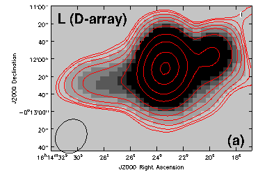
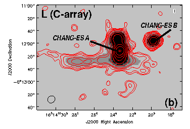
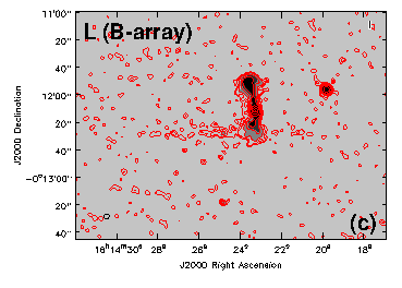
Figure 1: L-band images of UGC 10288 (both greyscale and contours). The beam size is shown as a black ellipse at the bottom left and corresponding map parameters are given in Table 3. (a) D-array map; contours are at 84 (2$\sigma$), 120, 200, 350, 600, 1200, 3000, 6000, 12000, and 18000 $\mu$Jy beam^-1. (b) C-array map; contours are at 44 (2$\sigma$), 60, 90, 150, 200, 400, 800, 1600, 3000, 6000, and 12000 $\mu$Jy beam^-1. The background source is labelled. (c) B-array map; contours are at 28 (2$\sigma$), 50, 100, 200, 400, 1200, 3600, and 8000 $\mu$Jy beam^-1.

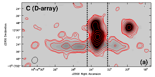
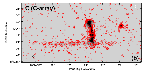
Figure 2: C-band images of UGC 10288 (both greyscale and contours). The beam size is shown as a black ellipse at the bottom left and corresponding map parameters are given in Table 3. (a) D-array map; contours are at 14 (2$\sigma$), 20, 40, 80, 150, 300, 600, 1200, 3000, and 6000 $\mu$Jy beam^-1. Dashed lines denote the region used to estimate the fluxes of Table 5. (b) C-array map; contours are at 6.2 (2$\sigma$), 12, 20, 30, 60, 120, 200, 400, 1600, and 6000 $\mu$Jy beam^-1.

In brief, we used the wide field imaging algorithm (Cornwell, Golap, & Bhatnagar, 2008) and multi-scale, multi-frequency synthesis (ms-mfs) during imaging (Cornwell, 2008; Rau & Cornwell, 2011). Wide field imaging takes into account the fact that all antennas may not be co-planar. The multi-scale clean assumes that the emission can be represented by a variety of spatial scales, rather than only point sources as has been largely done in the past. Multi-frequency synthesis makes use of the fact that, at different frequencies within the band, the uv spacings (measured in k$\lambda$) are also different and therefore the uv plane is more filled in than would be the case for monochromatic observations. We also fit the emission across the band in each pixel with a spectrum (Sault & Wieringa, 1994) of the form, $I_{\nu}\,\propto\,\nu^{\alpha}$, which, in practice, is expanded as a Taylor series with 2 terms (see Paper 2). At the end of the cleaning process, the image is constructed by reconvolving the clean components with a Gaussian of the same full-width-half-maximum (FWHM) as the dirty beam.

Each data set was then self-calibrated (e.g. Pearson & Readhead, 1984), with the exception of D-array L-band for which self-calibration attempts did not improve the map. The number and type of self-calibration iterations is given in Table 3.

The resulting total intensity images are seen in Figs. 1 and 2 for the L-band and C-band data, respectively. We additionally formed images (not shown) at spatial resolutions intermediate between those shown in these figures (e.g. by tapering the uv plane response). The images of Figs. 1 and 2 are shown without a primary beam correction, but any flux density (or other numerical) measurements are made on primary beam-corrected images. The primary beam correction was carried out as described in Paper 2, except that the beam has now been constructed with frequency weighting that matches the frequency weighting of the data (for example, the weighting that necessarily results from flagging)

2.4 Polarization Calibration and Imaging

Polarization calibration proceeded in the same fashion for all data sets. The cross correlation data (RL and LR) were first inspected separately and additional flagging was carried out as needed. A known model for Stokes Q and U for the primary calibrator was introduced, based on formulae given in Paper 2. The relative antenna-based delay correction between R and L was then derived using the primary calibrator. The leakage terms between the R and L circularly polarized feeds were found from the polarization leakage calibrator (Table 2). Finally, the absolute polarization position angle on the sky was determined from the known position angle for the primary calibrator ($\chi\,=\,33^{\circ}$ for 3C 286). During each of these steps, all previously determined calibration tables were applied on the fly. Finally, all calibration tables, including the self-calibration table determined from the corresponding total intensity map, were applied to the RL and LR data.

Imaging of Stokes Q and U proceeded in the same fashion as for I but the largest spatial scale was dropped during cleaning (except for D-array L-band) since the extent of the polarized emission is not as great as in total intensity. Maps of polarized intensity were then formed for each array and frequency, correcting for the bias introduced by the fact that P images do not obey Gaussian statistics (Simmons & Stewart, 1985; Vaillancourt, 2006). Maps of E vectors rotated by 90^∘ were also formed after first blanking all emission less than 3$\sigma$, where $\sigma$ is the rms noise of the respective Q and U maps, resulting in an uncertainty of $\pm$ 10 degrees. These vectors would be equivalent to the intrinsic direction of the regular magnetic field, B, if there were no Faraday rotation. The maps of polarized intensity (without primary beam corrections) superimposed with the rotated E vectors are shown in Figs. 3 and 4.

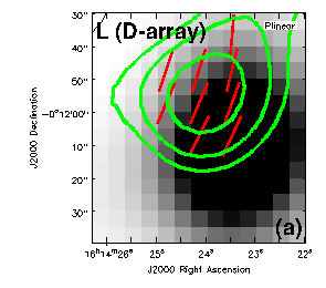
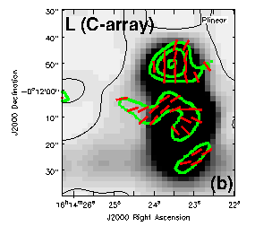
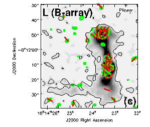
Figure 3: L-band polarization images of UGC 10288 (green contours) with E vectors rotated by 90^∘ (red, formed where Q and U $>$ 3$\sigma$). The greyscale represents the corresponding total intensity (I) image along with its 2$\sigma$ contour (black) from Fig. 1. Map parameters are given in Table 3, except that the D-array polarization image has been made from Q and U data that have been smoothed slightly to match the corresponding I data. (a) D-array map; contours are at 105 (3$\sigma$), 150, and 220 $\mu$Jy beam^-1. (b) C-array map; contours are at 65.1 (3$\sigma$), 110, and 175 $\mu$Jy beam^-1. (c) B-array map; contours are at 38.1 (3$\sigma$), 90, and 175 $\mu$Jy beam^-1.

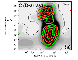
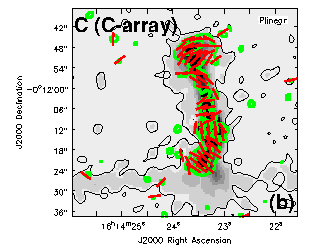
Figure 4: C-band polarization images of UGC 10288 (green contours) with E vectors rotated by 90^∘ (red, formed where Q and U $>$ 3$\sigma$). The greyscale represents the corresponding total intensity (I) image along with its 2$\sigma$ contour (black) from Fig. 2. Map parameters are given in Table 3. (a) D-array map; contours are at 16.2 (3$\sigma$), 35, 70, and 120 $\mu$Jy beam^-1. (b) C-array map; contours are at 8.7 (3$\sigma$), 30, 75, and 140 $\mu$Jy beam^-1.

2.5 Combined Array/Frequency Images and Spectral Index Map

The uv data at each frequency (B, C, and D arrays at L-band and C and D arrays at C-band) were combined in order to obtain higher S/N and more complete uv coverage for each of the bands. The results of these combinations are parameterized in Table 4 and each map was also corrected for the primary beam as described above. We will refer to them as needed.

The power and versatility of CASA, moreover, along with the multi-array and frequency observations that we have carried out also allow us to form a single image from all arrays and frequencies. The self-calibrated uv data from all five observations are input into the clean algorithm and, with a point-by-point fit of the spectral index, an image can be made that corresponds to a frequency which is intermediate between L-band and C-band, i.e. at $\nu\,=\,$4.13 GHz. This process is time-consuming but produces a final image with improved sensitivity to spatial scales and, on average, lower rms. We show the result in Fig. 5, where the two images differ only in the uv weighting function adopted.

Since the spectral index, $\alpha$ ($I_{\nu}\,\propto\,\nu^{\alpha}$), is fitted during the imaging, a map of $\alpha$ has also been formed (see Paper 2 for details) and is shown in Fig. 10 along with its error map. A 3$\sigma$ cutoff has been applied to the data when forming the $\alpha$ map and the result has been corrected for the spectral index of the primary beam. The error map represents random errors at each point as described in Rau & Cornwell (2011) (their Eqn. 39). Note that similar spectral index maps were formed for each individual data set as well (Sect. 2.3), but we show only the combined array/frequency result because of its higher S/N. In principle, it is also possible to solve for curvature in the spectral index (see Paper 2 for examples); however, the uncertainties become large, given the S/N in the disk of UGC 10288, and we did not pursue this for UGC 10288.

The remaining issue is to consider whether there might be missing flux from a lack of short spacings. At L-band, we detect all spatial scales less than 16 arcmin and, at C-band, less than 4 arcmin. The optical galaxy is 4.9 arcmin in diameter (Table 1) but, as illustrated in Figs. 1 and 2, the radio diameter does not extend beyond $\approx$ 3 arcmin. Moreover, we do not observe any ‘negative bowls’ around the emission, as would be the case if there were missing spacings. Consequently, there should be no missing flux in these data.

3 Results

3.1 The Total Intensity Emission

A remarkable result of these observations is the discovery of a strong, double-lobed extra-galactic radio source (EGRS) which is most certainly in the background of the UGC 10288 field. Previous to these observations, the only radio continuum images obtained were of the galaxy and background source blended together (see Hummel, Beck, & Dettmar, 1991; Condon et al., 1998). Indeed, the previously measured flux density from the combined sources, $S_{1.4~{}GHz}$ = 26.1 mJy (Condon et al., 1998) met our minimum flux density criterion (23 mJy) for membership in the CHANG-ES survey (Paper 1); however, it would have fallen far below that cut-off, had a measurement existed for the galaxy alone.

We now see both the galaxy and the background source in detail. There is an optical point source at the core of the EGRS (Fig. 5), with Sloan Digital Sky Survey (SDSS) DR9 identifer, J161423.28-001211.8, listed as a galaxy with a photometric redshift of $z_{phot}$ = 0.388 $\pm$ 0.026. We have named this background source, CHANG-ES A, and labelled it in Fig. 1b. Another strong source (CHANG-ES B, labelled in Fig. 6) is blended with the disk of UGC 10288 in D-array L-band (Fig. 1a), making the UGC 10288 disk appear to be skewed towards the north-west in that figure. CHANG-ES B also has an optical background galaxy at its center, namely J161419.79-001155.6 at $z_{phot}$ = 0.39 $\pm$ 0.11, in agreement with the redshift of CHANG-ES A. Therefore CHANG-ES A and CHANG-ES B possibly form a background pair.

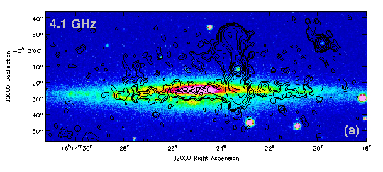
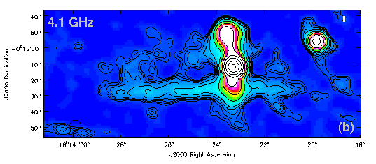
Figure 5: Total intensity combined array images of UGC 10288 (all arrays, both bands) corresponding to a frequency, $\nu_{0}\,=\,4.1$ GHz, shown at two different uv weightings. (a) I contours of the higher resolution Briggs robust = 0 uv weighting at 14 (2$\sigma$), 20, 30, 56, 100, 200, 400, 800, 2000, and 4000 $\mu$Jy beam^-1 over the Sloan Digital Sky Survey (SDSS) r band colour image. The beam size ($\sim$ 3.5 arcsec, Table 4) is shown at lower left. (b) I contours and colour of the lower resolution Briggs robust = 0 + 16 k$\lambda$ uv tapered image, with contours at 20 (2$\sigma$), 25, 30, 38, 55, 80, 160, 300, 600, 1200, 2400, 4800, and 8500 $\mu$Jy beam^-1. The beam size ($\sim$ 6.5 arcsec, Table 4) is shown at lower left.

3.1.1 Flux Densities and Global Spectral Index

Estimates of the flux densities of the various sources are given in Table 5. All flux densities were measured from the primary-beam corrected C-array L-band (Fig. 1b) and D-array C-band (Fig. 2a) maps. For both bands, the total flux density of UGC 10288 and CHANG-ES A were measured together. Then the flux density of CHANG-ES A was estimated from a measurement within the two dashed lines shown in Fig. 2a, a width of 34 arcsec. The flux density of UGC 10288 alone was then measured in a region of equivalent width to the east of CHANG-ES A along the galaxy’s disk. Assuming that this measured flux density is approximately equivalent to the flux density of UGC 10288 within the box occupied by CHANG-ES A, it was then subtracted from the CHANG-ES A measurement as a correction for the contribution of the galaxy’s disk within the dashed lines. At L-band, this correction amounted to 4% of the flux density of CHANG-ES A, and 22% of the flux density of UGC 10288. At C-band, the correction constituted 4% of the flux density of CHANG-ES A and 32% of the flux density of UGC 10288. In addition, at L-band, the totals were then summed and compared to the combined, blended emission from all three sources, i.e. UGC 10288, CHANG-ES A and CHANG-ES B as measured in the D-array L-band image (Fig. 1a); the totals agree to within 0.5%.

The global spectral index of UGC 10288 was calculated from the flux densities as just described, the result given in Table 5. The two sources are both clearly dominated by non-thermal emission.

3.1.2 The Star Formation Rate of UGC 10288

It is remarkable that UGC 10288 reveals extra-planar emission (see next two subsections) when the total flux density is only a few mJy. This leads us to consider the star formation rate (SFR) of the galaxy, since halo emission is often associated with such activity.

UGC 10288’s SFR_IRAS of 1.3 M_⊙ yr^-1 as given in Table 1, has been calculated from Infrared Astronomical Satellite (IRAS) data (Paper 1), but, like the radio continuum, the IR emission will certainly be contaminated by emission from CHANG-ES A.

A closer inspection of the IRAS flux densities, moreover, suggests foreground contamination as well. Given the observed IRAS 60 to 100 $\mu$m flux density ratio of UGC 10288 ($f_{(60\,\mu m)}/f_{(100\,\mu m)}$ = 0.236), the galaxy appears to be extremely cold. In fact, this flux density ratio is $\approx$20% smaller (colder) than that for the most extreme (coldest) galaxy included in the Dale & Helou (2002) spectral energy distribution (SED) models of normal star-forming galaxies. If CHANG-ES A is indeed a background radio galaxy, we naively would not expect it to be colder than all galaxies in the local Universe. If anything, we would expect a warmer temperature arising from hot dust being powered by the accreting black hole. Therefore, it seems that the most likely explanation for the cold dust temperature is significant contamination by difficult-to-remove foreground cirrus emission that is contributing to the IRAS flux densities.

Given these issues, an alternative approach is to use the calibrated, known radio continuum - FIR relation to estimate the SFR of UGC 10288 from its radio continuum emission as estimated in Sect. 3.1.1 with CHANG-ES A’s flux density subtracted. For this, we adopt the calibrations of Murphy et al. (2011) which use a Kroupa initial mass function (IMF) and a supernova cutoff of 8 M_⊙.  The SFR estimated from the thermal radio continuum requires an electron temperature which we take to be 10⁴ K. The SFR estimated from the non-thermal radio continuum requires a knowledge of the non-thermal spectral index, $\alpha_{NT}$, whereas we have, from the observed flux densities of Table 5, a global spectral index of $\alpha\,=\,-0.76$, using the convention,  ($S_{\nu}\,\propto\,\nu^{\alpha}$).

However, we can estimate $\alpha_{NT}$ by combining the thermal and non-thermal calibrations of Murphy et al. (2011) (their Eqns. 11 and 14) and the constraint that the measured flux density is the sum of the non-thermal and thermal flux densities at any frequency. i.e.

$$\frac{S_{\nu_{1}}}{S_{\nu_{2}}}\,=\,\left(\frac{\nu_{1}}{\nu_{2}}\right)^{\alpha_{NT}}\frac{\left[0.144\,(\nu_{1})^{-\alpha_{NT}-0.1}\,+\,1\ \right]}{\left[0.144\,(\nu_{2})^{-\alpha_{NT}-0.1}\,+\,1\ \right]}$$ (1)

where $S_{\nu}$ is the total flux density at frequency, $\nu$ and these calibrations assume a linear dependence of SFR on both thermal and non-thermal luminosity. The use of this equation infers a thermal/non-thermal fraction which has a dependence on both frequency and $\alpha_{NT}$.

Using our measured flux densities of Table 5 at two frequencies, we can solve Eqn. 1 to find $\alpha_{NT}\,=\,-1.04$. This leads to a thermal to total and non-thermal to total flux density in L-band of, ${(S_{T}/S)}_{1.5}\,=\,0.17$, ${(S_{NT}/S)}_{1.5}\,=\,0.83$, respectively.  In C-band, the results are ${(S_{T}/S)}_{6.0}\,=\,0.44$, ${(S_{NT}/S)}_{6.0}\,=\,0.56$, respectively.

Finally, with the SFR calibration (eqn. 15 of Murphy et al., 2011), we find SFR = 0.51 M_⊙ yr^-1.

We caution that, if the non-thermal luminosity, $L_{NT}\,\propto\,$SFRⁿ, where $n\,>\,1$ (e.g. n$\,=\,1.3$ Niklas & Beck, 1997), then there would be a weak dependence on SFR on the right hand side of Eqn. 1; the adjustment, however, does not significantly perturb the above results.

This newly determined SFR is considerably lower than the original SFR which was found from IRAS values and should be  more accurate since it corrects for the contribution of CHANG-ES A and also uses a  spectral index determined from the data. If, instead, we use the global FIR-radio continuum relation (Eqn. 17 of Murphy et al., 2011) based on earlier calibrations (de Jong et al., 1985; Helou, Soifer & Rowan-Robinson, 1985), then SFR = 0.39 M_⊙ yr^-1. In either case, the radio-derived SFRs are clearly much lower than the IRAS-based estimate of 1.3 M_⊙ yr^-1.

In summary, the SFR based on IRAS photometry (Table 1) neither corrects for the strong contribution from CHANG-ES A nor for contamination from foreground cirrus. We estimate that a value between 0.4 and 0.5 M_⊙ yr^-1 is a more accurate estimate of the true SFR in UGC 10288. Note that the range given here is dominated by the assumptions that have been made, rather than by a formal error determination. This galaxy is now one of the lower SFR galaxies in the CHANG-ES sample (Paper 1).

3.1.3 Foreground/Background Point-like Sources

Fig. 6 shows the combined C+D array C-band map of UGC 10288 overlaid on the $\lambda$ 3.6 $\mu$m image from the Spitzer Space Telescope. These radio data have the lowest rms of all combined data sets (Table 4) as well as high resolution. Comparing with the Spitzer image, which was chosen because it should show both foreground stars as well as background quasars, should reveal how much radio emission (especially in regions of apparent halo features) is associated with point-like sources in the displayed field.

We searched for sources for which both the IR and radio emission are point-like and for which the radio emission is sufficiently separated from the disk of UGC 10288 to allow a discrete measurement of flux density. The process was then repeated for the combined B+C array L-band map (not shown), although the latter image has almost 4 times higher rms noise than at C-band for approximately equal beam sizes. The resulting sources are labelled in Fig. 6 and their properties listed, along with SDSS identifiers (where available) in Table 6.

Let us consider the region that is encompassed by the box shown in Fig. 6 (16^h 14^m 25.9^s $\leq$ RA $\leq$ 16^h 14^m 28.9^s; -00^∘ 12^′ 21^′′ $\leq$ DEC $\leq$ -00^∘ 11^′ 40^′′). This box contains significant ‘halo’ emission in the form of a large extended arc-like feature visible in the all-data image of Fig. 5b. This arc extends to a height of 21 arcsec (3.5 kpc) above the plane. The flux density contained within this box is $S_{4.1~{}{\rm GHz}}\,=\,450~{}\pm~{}80$ $\mu$Jy. Only one identified point-like source (Source 2) is located within this region whose flux density, extrapolated to 4.1 GHz, is $<$ 16 $\mu$Jy (Table 6). Consequently, although we cannot conclude that the arc-like feature represents a single coherent structure, its flux density does not result from background sources. Hereafter, we will refer to this features as the ‘arc’ for simplicity.

There is also a feature extending to the north on the west side of the galaxy (at RA $\approx$ 16^h 14^m 21.5^s, DEC $\approx$ -00^∘ 12^′ 12^′′) as shown in Fig. 5b; but there are no point sources meeting our criteria in this region at all.

We caution that if a background source displays double-lobed radio structure, then it could be displaced with respect to the IR source and might have been missed in this search, as would objects with weak IR flux and those that are blended with the disk. However, even if we increased our point-like source flux density estimate by a factor of two, its contribution to the flux density of halo features in UGC 10288 would still be negligible. By including other array configurations in the maps, in particular short spacings, the sensitivity to extended halo features is enhanced but there should be no change in sensitivity to point sources.

It is beyond the scope of this paper to examine in detail the nature of the point-like sources. SDSS identifiers, where available, indicate that three of the four identified sources are stars which would be an interesting result given the detected radio emission. However, one of these sources (Source 5, SDSS J161424.84-001318.3) although labelled as a star, has SDSS colours (u-g = +0.18, g-r = -0.18, r-i = 0.45, i-z = -0.07) which are entirely consistent with those of a quasar over a range of redshift (Pâris et al., 2012, their Fig. 28).

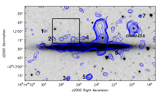
Figure 6: Combined C and D array C-band contours over a greyscale $\lambda\,$3.6 $\mu$m map from the Spitzer telescope. Contour levels are at 8 (2$\sigma$), 11, 15, 20, 30, 50, 100, 300, 600, 1200, and 3000 $\mu$Jy beam^-1, and the beam size ($\sim$ 6 arcsec, Table 4) is shown at lower left. Several point sources showing radio emission that are distinct from the disk of UGC 10288 have been numbered (Table 6). The box encloses a region containing the radio continuum extension seen in Fig. 5b.

3.1.4 Comparison with Images at other Wavebands

It is apparent that halo radio emission is associated with UGC 10288. Here, we appeal to ancillary data, where available, to shed further light on the high latitude features.

Few resolved images of UGC 10288 are available at other wavebands but, of those available, we show several overlays in Figs. 7 and 8. Fig. 7 shows our all-array and all-frequency radio continuum images of Fig. 5 superimposed on the H$\alpha$ image of Rand (1996). In Fig. 8, we show contours from the Wide-field Infrared Survey Explorer (WISE) (Wright et al., 2010) at $\lambda\,$12 $\mu$m and $\lambda\,$22 $\mu$m over H$\alpha$ emission and our L-band combined array image, respectively. In each overlay, the spatial resolutions of the two images are identical.

Because radio emission from UGC 10288 is blended with that of CHANG-ES A, it is difficult to disentangle which source is responsible for specific features observed at locations close (in projection) to that background source. For example, a horizontal feature appears to emanate from the northern lobe of CHANG-ES A towards the east (see RA $\sim$ 16^h 14${\rm m}$ 25^s, DEC  $\sim$ -00^∘ 12^′ 06^′′ in Fig. 7b). There is also a projection which extends to the south of CHANG-ES A’s southern radio lobe (RA $\sim$ 16^h 14${\rm m}$ 235^s, DEC  $\sim$ -00^∘ 12^′ 43^′′ in Fig. 7b) and farther south as a narrower radio extension in Fig. 8b). Neither of these have obvious counterparts at other wavebands, although the southern feature appears to lie between two H$\alpha$ extensions (see below).

The IR emission does not distinguish between UGC 10288 and background sources either, since for example, the bright background radio source, CHANG-ES B, to the west of CHANGES-A (marked in Fig. 6) is also an IR emitter at both $\lambda\,$12 and 22 $\mu$m.

As we have no way to determine the origin of radio continuum features near CHANG-ES A, we will concentrate instead on other features that are farther from this region and are more likely to be associated with UGC 10288. The H$\alpha$ emission is helpful in this regard, since it clearly has an origin in UGC 10288 itself.

We must also note that each of the images suffers from some low-level artifacts.

For the radio images, the map contains residual sidelobes which, for the most part, we have included in measuring and quoting rms map values. However, residual sidelobes from a source 6.3 arcmin to the east of UGC 10288 are likely responsible for the horizontal feature at the south-east side of Fig. 7b (RA $\sim$ 16^h 14^m 30^s, DEC  $\sim$ -00^∘ 12^′ 50^′′), and residual sidelobes from another point source 6.2 arcmin to the south-west may be responsible for the faint greyscale NE-SW feature visible on the west side of Fig. 8b (RA $\sim$ 16^h 14^m 17^s, DEC  $\sim$ -00^∘ 12^′ 15^′′).

Similarly, in the H$\alpha$ image, it has been noted that the galaxy’s bulge has been oversubtracted (Rand, 1996). And both WISE images show broad (arcmin scale) NE-SW striping which may be producing or contributing to the broad southward extension at RA $\sim$ 16^h 14^m 30^s, DEC  $\sim$ -00^∘ 12^′ 50^′′ (Fig. 8a).

In any following discussion, therefore, we will keep these cautions in mind and discuss results that appear to be robust to such artifacts. Fig. 7a shows the highest resolution ($\sim$ 3.5 arcsec) radio/H$\alpha$ overlay with arrows pointing to specific features. Discrete in-disk H$\alpha$ emission reveals specific sites of unobscured star formation.

Feature 1 is a discrete star forming region in the disk above which there is a vertical plume of H$\alpha$ emission (to the north). The H$\alpha$ plume is more readily seen in the smoothed map of Fig. 7b and has a $\lambda\,$12 $\mu$m counterpart (Fig. 8a). No radio emission can be confirmed in this plume, but a slight extension visible in L-band greyscale image of Fig. 8b is close to its location, slightly displaced to the east. That is, the radio extension’s location is more closely aligned with the gap immediately to the east of star forming region #1.

Feature 2 refers to several star forming complexes that are located below the strong northward radio plume seen in Fig. 7. The two arrows point to gaps in the H$\alpha$ in-disk emission, the easternmost one also corresponding to a gap in the in-disk radio emission. Two ‘prongs’ in the radio emission close to the disk (Fig. 7b) are immediately above these gaps.

The southern H$\alpha$ extension of feature 3 was originally pointed out by Rand (1996) and is in a region of low brightness in comparison to the star forming regions to the east and west of it. This feature shows a small northwards elongation in the radio at high resolution (Fig. 7a).

Feature 4 points to another gap in the H$\alpha$ emission between two star forming regions. There is a small radio extension to the north that is visible in the high resolution image (Fig. 7a) but a much larger corresponding radio continuum feature can be seen at lower resolution (Fig. 7b).

Finally, feature 5 refers to two southwards prongs which were originally identified by Rand (1996) who also noted a ‘hemispherical’ shape formed by these two features together. We have not detected any high-latitude radio emission associated with this feature.

In summary, our high resolution data suggest that radio continuum features are more likely to be seen above in-disk gaps in the H$\alpha$ emission.

It should be pointed out, of course, that apparent correlations above an edge-on disk could apply to any location along the line of sight (although such indeterminacy is less severe at large galactocentric radii). This means that such apparent correlations do not necessarily represent physical correlations. Nevertheless, the observed trend is worth pointing out, since it is rare that an edge-on galaxy has adequate data to compare H$\alpha$ and radio continuum results at the same resolution with good sensitivity. A similar anti-correlation has been observed before between in-disk H$\alpha$ emission and high latitude radio continuum features in NGC 5775 (Lee et al., 2001). We discuss this further in Sect. 4.

On broader scales, it is more difficult to associate high latitude radio emission with in-disk activity. Intriguing features are a south-wards H$\alpha$ arc seen in Fig. 7b at RA $\sim$ 16^h 14^m 24.5^s, DEC $\sim$ -00^∘ 12^′ 48^′′, and a possible companion feature at RA $\sim$ 16^h 14^m 22.7^s, DEC $\sim$ -00^∘ 12^′ 42^′′ between which the southern radio continuum extension, mentioned above, lies. In Fig. 8a, the $\lambda\,$12 $\mu$m emission shows several other northwards extensions as well as a south-wards arc-like feature on the east side of the galaxy, and in Fig. 8b, and a southwards radio extension seen at L-band on the far east end of the disk.

We note two other observations regarding the distributions.

The first is the north-south radio asymmetry observed on the east side of the major axis, best seen in Fig. 7b. i.e. there is a large arc-like extension towards the north but nothing equivalent to the south. This may reflect N/S asymmetries in star forming regions and/or N/S density asymmetries in the disk. Such asymmetries can also be produced by ram pressure as a galaxy moves through an intergalactic medium; this is possible for UGC 10288, given that it is in a sparse group (Sect. 1), but we have no independent observations that would argue for or against this speculation.

The second observation is that UGC 10288 does not appear to have a global radio halo, but rather it has discrete high latitude radio extensions. Table 7 compares beam-corrected exponential scale heights between the 4.1 GHz all-data map (Fig. 5b) and both the H$\alpha$ and WISE $\lambda\,$12 $\mu$m data at the same (7 arcsec) resolution according to the method of Dumke et al. (1995). The fitting has been carried out for data that have been averaged in strips, each 26.4” = 1.76 s wide, that are labelled in Fig. 7b. The values are from single-exponential fits that apply to the disk (for example, for Strip #2 North, the horizontal feature at DEC $\sim$ -00 12 06, was avoided). Note that the strips that do not have significant extensions (mainly #2 South but also #1 South and #2 North) have low to modest scale heights in radio continuum (0.46, 0.85 & 0.86 kpc, respectively), whereas the strips containing discrete extensions (#1 North & # 4 North/South) are wider in z, on average (1.3, 1.4, & 1.1 kpc, respectively) as would be expected. See Sect. 4 for more discussion.

In order to give an overview of the relative spatial distributions of the various sources of emission, we finally display a multi-frequency image (Fig. 9) in which several data sets have been overlayed with different colours (see caption). Our radio data show CHANG-ES A and CHANG-ES B in cyan; our masking technique (Rector et al., 2007) allows us to show their optical counterparts (yellowish) at their cores. The disk of UGC 10288 looks quite wide vertically in this picture because of the WISE $\lambda\,12~{}\mu$m image. For more information as to the techniques used to combine the data sets, see Rector et al. (2007).

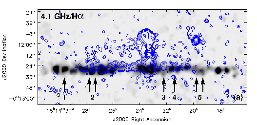
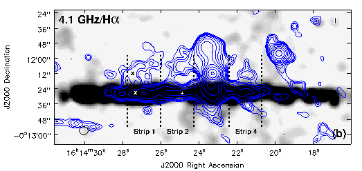
Figure 7: Contours from Fig. 5 over the H$\alpha$ emission measure map of Rand (1996) smoothed to the same resolution as the radio data in each case. The beam size is shown at bottom left. (a) Contours are from Fig. 5a and the resolution is $\sim$ 3.5 arcsec (Table 4). The arrows point to features discussed in Sect. 3.1.4.(b) Contours are from Fig. 5b and the resolution is $\sim$ 6.5 arcsec, Table 4). A plus marks the center of UGC 10288 and two crosses mark the positions discussed in Sect. 3.3.1. The labelled strips are discussed in Sect. 3.1.4.

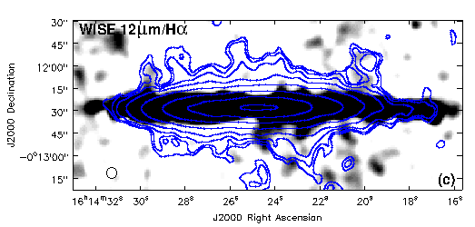
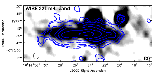
Figure 8: (a) Contours (in arbitrary units) of the WISE $\lambda\,$12 $\mu$m image over the H$\alpha$ image of Rand (1996), both smoothed to 7.0 arcsec resolution (beam shown at lower left). (b) Contours (in arbitrary units) of the WISE $\lambda\,$22 $\mu$m image over the combined BCD array L-band data (original information given in Table 4) smoothed to the same 12 arcsec resolution as the WISE data (beam at lower left).

Figure 9: Multi-frequency colour image of the UGC 10288 field showing our C-array C-band image (Fig. 2b) in cyan, the combined all-array, all-frequency image in darker cyan (Fig. 5b), the WISE $\lambda\,12~{}\mu$m image (Fig. 8a) in orange, the Spitzer $\lambda\,3.6~{}\mu$m image (Fig. 6) in yellow, the H$\alpha$ image of Rand (1996) Fig. 7 in rose, the SDSS r band image (Fig. 5a) in blue and the SDSS g band image in purple. Smoothing, colour choice and masking follow the techniques described in Rector et al. (2007). Spatial resolutions vary and have been chosen for visual effect. Both CHANG-ES A and CHANG-ES B (cyan and darker cyan at lower resolution) are quite obvious, and the large vertical width of the disk which appears salmon coloured at the edges, is due to the large width seen in the WISE $\lambda\,12~{}\mu$m image.

3.2 Spectral Index

The spectral index map along with a point-by-point error map (see Sect. 2.5) are shown in Fig. 10. The disk of UGC 10288 is of course blended with CHANG-ES A which shows the classic signature of a double-lobed radio source: a flatter spectral index at the center and steeper in the lobes.

The spectral index in the disk of UGC 10288 shows complex structure but, as also shown by the global spectral index (Sect. 3.1.1), non-thermal spectra dominate (Table 5). At the locations of the three brightest star forming regions in the disk (denoted with crosses), as identified from the H$\alpha$ map, the spectral indices are $\alpha\,=\,-0.7~{}\pm~{}0.3$, $\alpha\,=\,-0.4~{}\pm~{}0.2$, and $\alpha\,=\,-0.1~{}\pm~{}0.3$ from east to west, respectively. If averaged over a beam rather than measured at the H$\alpha$ peak, these values become $\alpha\,=\,-0.8~{}\pm~{}0.3$, $\alpha\,=\,-0.4~{}\pm~{}0.2$, and $\alpha\,=\,-0.3~{}\pm~{}0.2$ from east to west, respectively. Thus, only the westernmost SF region is consistent with a purely thermal spectrum at its peak. However, if we insist that the SFR calibrations discussed in Sect. 3.1.2 hold at every point, then a flatter observed spectral index actually implies a flatter non-thermal spectral index, presumably reflecting a younger cosmic ray electron population. Such details will be explored in future CHANG-ES papers.

Note that these 3 star forming regions do not align exactly with the flattest spectral indices. The region with the flattest spectral index is directly north of the central star forming region and there is another region of flatter spectral to the south-west of the westernmost star forming region. This could be a result of outflows in these regions; such spectral index flattenings have been observed before in regions of outflows (e.g. NGC 5775, Lee et al., 2001). However, it is important to keep in mind the uncertainties on these quantities. Generally, the errors also increase towards the edges of the map.

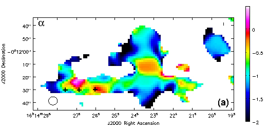
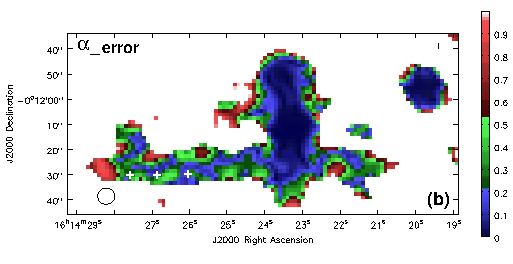
Figure 10: Spectral index map, $\alpha$ (a), and uncertainty in the spectral index (b) (random errors only), made from all data (all arrays, both bands) corresponding to the uv weighting image of Fig. 5b ($S_{\nu}\,\propto\,\nu^{\alpha}$) with a 3$\sigma$ intensity cutoff applied. The 3 brightest star forming regions from Fig. 7a have been marked with crosses and the beam is shown at lower left. Several points from the $\alpha$ map have uncertainties that appear white because they have values that are $>$ 1. The beam size ($\sim$ 6.5 arcsec, Table 4) is shown at lower left.

3.3 Polarization

3.3.1 Polarization Images and Sample Magnetic field

Figs. 3 and 4 show the polarization maps at L-band and C-band, respectively. We do not detect polarization in the disk of UGC 10288 in the individual observations. Rather, it is the background radio source, CHANG-ES A, that shows polarization. Although a more complete analysis of the polarization-related properties awaits a future paper, a few results are presented here.

For both B-array, L-band (resolution $\sim$ 3.6 arcsec) and C-array, C-band (resolution $\sim$ 3.0 arcsec) the highest polarization occurs right at the core of CHANG-ES A (peak values and resolutions provided in Table 3). At this location, the percentage polarization at L and C bands is 1.9% and 2.0%, respectively.

North and south of the core, although the polarized intensity is lower, the percentage polarization increases. At the peak polarization position of the C-band data in the northern lobe, for example, the values are 17% and 30% at L and C bands, respectively (RA = 16^h 14^m 23.7^s, DEC = -00^∘ 11^′ 48^′′). At the southern peak position, the corresponding values are 6.3% and 31% at L and C bands, respectively (RA = 16^h 14^m 23.47^s, DEC = -00^∘ 12^′ 21^′′).

The L-band percentage polarization is weaker than at C-band, as expected, since more Faraday de-polarization occurs at the lower frequency, either intrinsic to the source or contributed via UGC 10288 or both. Moreover, the L-band value is lower still for the southern lobe, compared to the northern, likely because of stronger Faraday depolarization in the (possibly turbulent) disk of UGC 10288. The fractional polarization in the core is much lower than in either lobe; this is not unusual for double-lobed radio sources (e.g. Rudnick, Jones, & Riedler, 1986; Saikia & Kulkarni, 1998) suggesting that much of the core/lobe difference is intrinsic to CHANG-ES A.

UGC 10288 does not lend itself well to global magnetic field calculations, given the interfering presence of CHANG-ES A. However, we have taken two sample positions, one in the disk, and one in the large northern arc on the east side of UGC 10288 visible in the 4.1 GHz map, to estimate the total minimum energy magnetic field strength, $B$. We use the revised minimum energy formulae given in Beck & Krause (2005) for isotropic fields and adopt a proton-to-electron number density ratio of 100. The positions are marked with crosses in Fig. 7b, the disk position being immediately below the arc.

At the position in the eastern disk, a projected distance of $x\,=\,$39 arcsec from the center, $\alpha\,=\,-0.44\,\pm\,0.18$ and $I_{4.1~{}GHz}\,=\,70.4$ $\mu$Jy beam^-1. Then $\alpha_{NT}\,=\,-0.54$ and $I_{NT}\,=\,55.4$ $\mu$Jy beam^-1 by Eqn. 1 and the arguments presented in Sect. 3.1.2. For a line of sight distance of 6.0 kpc (estimated from a 1/e radial scale length) then the minimum energy magnetic field strength is $B\,=\,10\,\pm\,3$ $\mu$G. Here, the error represents measurement error only, which is dominated by the uncertainty in $\alpha$; it does not include errors that may be associated with the assumptions.

At the position in the northern extension, 15 arcsec above the plane (2.5 kpc in projection), $\alpha\,=\,-1.00\,\pm\,0.50$ (Fig. 10), $I_{4.1~{}GHz}\,=\,36.0$ $\mu$Jy beam^-1, we assume that the emission is dominantly non-thermal based on the absence of H$\alpha$ emission, and take $l\,=\,1.5$ kpc (9 arcsec) which is approximately the width of the arc at this location. Then, provided that the conditions for minimum energy are met for this region of steep spectral index, $B\,=\,12\,\pm\,5$ $\mu$Gauss, where, again, the error represents measurement error.

As Fig. 10 illustrates, there is considerable variation in spectral index (and its error) and the magnetic field strength will also vary with position. It is also not clear whether the thermal/non-thermal emission ratios follow the expectations of the calibrations of Murphy et al. (2011), point-by-point. Nevertheless, the approach in which the thermal/non-thermal ratio is tied to a SFR calibration, should be an improvement upon previous estimates for other galaxies which usually assume a constant and singular thermal/non-thermal ratio for every point in the galaxy. These preliminary calculations, then, suggest a total magnetic field strength of order 10 $\mu$G at the two sample positions selected.

3.3.2 Rotation Measures and the Regular Field

A powerful tool, which is potentially available for UGC 10288, is the technique of using the background radio galaxy, CHANG-ES A, to probe the foreground magnetic field. To this end, we computed the classical Faraday rotation measure (RM) map (Fig. 11) between the B-array L-band and the C-array C-band data, at 5 arcsec resolution. The maximum $1\sigma$ error is $\pm\,10$ rad m^-2 at the outer edge of each patch, while the $1\sigma$ error of the mean RM of Fig. 11 is $\pm\,2$ rad m^-2. The RM ambiguity is $\pm\,93$ rad m^-2.

The observed RM values are a superposition from CHANG-ES A, the galaxy UGC 10288, and the foreground of the Milky Way. The lobes of radio galaxies can have high RM values with a large dispersion, so that, when observed with low resolution, the average RM is small. The central sources of radio galaxies (jets) generally do not reveal significant intrinsic RM. The RM of CHANG-ES A’s northern lobe (at about 7 kpc projected distance above the plane of UGC 10288, marked ‘A’ in Fig. 11) of $+30\,\pm\,4$ rad m^-2 (average of the two visible regions) agrees well with the foreground RM of the Milky Way (Taylor, Stil, & Sunstrum, 2009; Oppermann et al., 2012) at the Galactic coordinates of our radio maps (l=+12^∘, b=+34^∘). This indicates that no correction for the RM ambiguity is needed.

The southernmost blob in Fig. 11 (marked ‘C’) is located behind the disk of UGC 10288, about 1.5 kpc above the plane, with an observed average value of RM$\simeq+62\,\pm\,4$ rad m^-2. We interpret the (foreground subtracted) value of RM${}_{i}\simeq+32$ rad m^-2 as indication of a regular magnetic field in the galaxy disk, pointing towards us. A line-of-sight component of about +2 $\mu$G, a thermal electron density of 0.02 cm^-3 and a path length of 1 kpc can provide the observed RM_i. If the path length is more than 1 kpc in the halo, the field strength and/or the electron density lowers by the same factor. However, as noted earlier (Sect. 3.1.4), when high latitude radio emission is observed, the features have generally been discrete with typical sizes of order a kpc. In addition, disk exponential scale heights are also typically $\approx$ 1 kpc. Consequently, at the location of ‘C’ at 1.5 kpc above mid-plane, we might expect the effective path length of the magnetic field to be approximately that of a typical high latitude discrete feature.

RM${}_{i}\simeq-7$ rad m^-2 (observed average value of RM$\simeq+23\,\pm\,2$ rad m^-2 for both parts) towards the central region of the radio galaxy, at about 3.5 kpc above the plane of UGC 10288 (‘B’), indicates that the field direction is reversed with respect to the plane. A thermal density in the halo of 0.01 cm^-3 requires a regular halo field with a line-of-sight component of about -1 $\mu$G, pointing away from us. Again, if the path length is more than 1 kpc in the halo, the field strength and/or the electron density lowers by the same factor. Between disk and halo, no regular field from the galaxy is detected, so that the RM is solely due to the Galactic foreground.

The conclusion that a field reversal is present depends, of course, on the accuracy of the RM measurements, especially region ‘C’ which is present in the total power maps only as diffuse emission between the core of CHANG-ES A and its southern radio lobe. If we use a higher cut-off of 3$\sigma$ to form the RM map, then the value of ‘C’ becomes 64 rad m^-1, rather than the 62 rad m^-2 seen in Fig. 11, i.e. within the quoted 1$\sigma$ uncertainty of $\pm$ 10 rad m^-2 on the RM at the map edges (see above). A 3$\sigma$ cut-off also reduces the 1$\sigma$ uncertainty in RM to $\pm$ 7 rad m^-2; however, such accuracy is not required for this conclusion.

A reversal between the azimuthal components of the disk field and halo field may be quite common among galaxies; it has been found from modeling the magnetic field in the Milky Way from extragalactic RMs (e.g. Sun et al., 2008; Jansson & Farrar, 2012) and also in the northern part of the galaxy M51 (Fletcher et al., 2011). Dynamo models can hardly explain such reversals if the same dynamo process operates in disk and halo, unless wind outflows allow such “mixed parities” (Moss et al., 2010).

These results are necessarily preliminary, but the fact that many spectral channels are available in each of our observations (Table 2) lends itself well to the application of the RM Synthesis technique (Brentjens & de Bruyn, 2005) to UGC 10288. This requires that (RA - DEC - Frequency) cubes be formed for all data sets, and is an approach that will be attempted in the future.

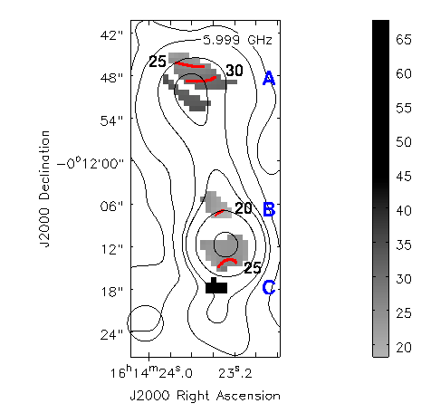
Figure 11: Rotation measure map, made from the L-band B-array and the C-band C-array data, at 5 arcsec resolution, computed at all pixels where the polarized intensities in both bands exceed twice the rms noise. Several contours (red) are marked, with all values in units of rad m^-2. The two regions with no contours marked have average values of 33 rad m^-2 (northern region) and 62 rad m^-2 (southern). Letters denote the regions discussed in Sect. 3.3.2. Black contours represent the 5 arcsec C-band C-array total intensity image at 6.2, 30, 150, 300, 1200, and 6000 $\mu$Jy beam^-1. The beam is marked at lower left.

4 Discussion

Our observations have revealed some new surprises in UGC 10288 and the multi-array, multi-frequency approach has been essential in understanding this galaxy and disentangling its emission from the background radio galaxy. Not only have we been able to correct for the emission of CHANG-ES A, but CHANG-ES B would also have been assumed to be part of UGC 10288 at low resolution (see Fig. 1a), had multiple arrays (i.e. higher resolutions) not been used.

Moreover, the combination of all arrays and both frequencies has allowed us to detect high latitude emission in UGC 10288. However, rather than having a broad scale halo, the high latitude features in UGC 10288 are discrete and, in the case of the arc-like feature seen extending towards the north on the eastern side of UGC 10288’s disk (Fig. 5b), also large. This feature extends to 21 arcsec ($~{}\sim$ 3.5 kpc) above the disk.

It is interesting to explore some properties of this arc. For example, taking the estimate of the total magnetic field strength ($B\,\sim\,10$ $\mu$G, Sect. 3.3.1) at the position marked in Fig. 7b (13.5 arcsec, or 2.2 kpc above the plane) and using standard formulae (e.g. Heesen et al., 2009), the particle lifetime to synchrotron losses is $t_{synch}\,\sim\,1.6\,\times\,10^{7}$ yr. We do not know the outflow velocity, but it must be substantial in order to detect synchrotron radiation at this $z$-height. For example, if there were no additional losses, this lifetime implies (for constant velocity) a vertical flow of $v_{z}\,\sim\,134$ km s^-1, and higher still if adiabatic or other losses are significant. The largest uncertainty, apart from those introduced by assumptions, belongs to $\alpha$ which affects $B$ by $\pm$ a few $\mu$G. Since $t_{synch}\,\propto\,B^{-3/2}$, then the uncertainty on $v_{z}$ due to the uncertainty on $\alpha$ alone is $\sim\,$30%. What we see, therefore, is that outflow speeds can be substantial in localized regions, even in galaxies with modest SFRs.

As pointed out in Sect. 3.1.4, the disk exponential scale heights in regions outside of the discrete high-latitude features is less than 1 kpc (Sect. 3.1.4, Table 7) and, even when one considers the scale height averaged over regions with and without radio extensions, the average is only $\approx$ 1 kpc. This lack of a global radio halo, we suggest, is consistent with a rather modest SFR in UGC 10288 which we have modified downwards to be 0.4 - 0.5 M_⊙ yr^-1. That is, discrete extensions may be formed in relation to underlying disk activity, but not globally. A comparison could be made to M 31 which has a similar (slightly lower) SFR of 0.3 M_⊙ yr^-1 (Arshakian et al., 2011) and for which the synchrotron exponential scale height is only $\sim$ 300 pc (Fletcher et al., 2004).

It is clear that galaxies with similar global SFRs can be quite different in other ways. For example, although the SFRs of M 31 and M 33 are similar, their star formation efficiencies, SFE = SFR/M(H₂), where M(H₂) is the molecular gas mass, differ by at least a factor of 3 (Tabatabaei & Berkhuijsen, 2010; Gardan et al., 2007, their Figs. 17 and 11, respectively). Similarly, galaxies with comparably low SFRs might show differences in the presence or absence of discrete high latitude radio continuum features. Possible reasons might be the degree of clustering of star forming regions, or the relative strength and direction of the magnetic fields.

When the various scale heights are averaged, irrespective of location, we find beam-corrected scale heights of $h_{e}({\rm 4.1~{}GHz})\,\sim\,1.0$ kpc, $h_{e}({n_{e}})\,\sim\,1.2$ kpc, where we have doubled the observed average H$\alpha$ scale height to take into account the fact that the observed emission measure $\propto$ $n_{e}^{2}$, and $h_{e}({12~{}\mu{\rm m}})\,\sim\,1.2$ kpc. Consequently the warm dust and thermal electron density scale heights are comparable and, arguably, so is the radio scale height, although the latter is far more irregular as Fig. 7b (from which the values of Table 7 were obtained) readily shows.

The high thermal fraction in UGC 1028 (44% in C-band, Sect. 3.1.2) also has been seen before, again in galaxies with low or modest SFRs. For example, Dumke et al. (2000) find a C-band thermal fraction as high as 54% for the galaxy, NGC 5907, and Chyzy et al. (2007) find thermal fractions of 50% to 70% in three late-type galaxies at 4.85 GHz compared to what is normally measured ($\approx$ 20%). These authors suggest that, in galaxies with higher SFRs, the non-thermal fraction increases because of the non-linear dependence of non-thermal luminosity on SFR, as noted in Sect. 3.1.2. Our results depend on an assumption of a linear dependence, but as already noted, we do not anticipate a significant change at the low SFR of UGC 10288 unless the non-thermal calibration is also markedly different. Consequently, our results of a high thermal fraction are consistent with previous estimates for galaxies with similar SFRs.

A significant new result is, of course, the detection of a double-lobed radio galaxy, CHANG-ES A, behind the disk of UGC 10288, which has allowed us to make some preliminary estimates of the regular magnetic field in UGC 10288 prior to a full Rotation Measure synthesis analysis. Aside from the Milky Way, there have been only a few limited examples in which polarized background sources have been used to probe foreground galaxies (Han, Beck, & Berkhuijsen, 1998; Mao et al., 2012) and these were for galaxies of large angular size (M 31 and the Large Magellanic Cloud). In the case of UGC 10288, which is only 4.9 arcmin in diameter, the 90 degree alignment of the double-lobed radio galaxy is so fortuitous that both the disk and halo regions of the foreground galaxy can be probed.

For an adopted electron density of $n_{e}\,=\,0.02$ cm^-3 a projected distance 1.5 kpc above the plane (position ‘C’ in Fig. 11) and a path length of 1 kpc, we find a regular field of $+$ 2 $\mu$G parallel to the line of sight. At 3.5 kpc above the plane (position ‘B’ in Fig. 11) with $n_{e}\,=\,0.01$ cm^-3, $B_{||}\,\sim\,-1$ $\mu$G, suggesting a reversal of the azimuthal field above the plane.

These values are still preliminary. Nevertheless, CHANG-ES A has the potential to be a powerful probe of both $B_{||}$ and $n_{e}$ in regions in which neither are measured directly via radio emission. At the lower position (‘C’), for example, the H$\alpha$ emission has already dropped to the level of the noise (Fig. 7a). This map has a 3$\sigma$ emission measure noise limit of 13 pc cm^-6 (Rand, 1996) which implies that any electron density less than $n_{e}\,=\,0.1$ cm^-3 over the same path length would not have been detected (adjusting as $1/\sqrt{l}$ for a different path length, $l$).

At the same time, our sampling of the total magnetic field strength in the discrete northern arc, 2.5 kpc above the plane, reveals a rather strong total magnetic field $B\,\sim\,10$ $\mu$G (Sect. 3.3.1). Although not at the same position as rotation measures were measured, the implication is that field strengths in discrete high latitude features could be similar to those in the disk, possibly because of field compression in the arc. A similar result was found for NGC 5775 (Soida et al., 2011) for which X-shaped extensions have fields almost as strong as in the disk, although the latter galaxy has, by contrast, a high SFR and global radio halo. NGC 4631 also has a relatively strong halo field (Hummel, Beck, & Dahlem, 1991). It is unlikely that discrete strong high latitude features could be a result of a mean-field dynamo alone. Localized SF activity in the underlying disk is likely contributing to this feature.

5 Conclusions

We have obtained JVLA wide-band radio continuum data of UGC 10288 in both total power as well as polarized intensity as part of the CHANG-ES program (Paper 1). Three different array configurations (B, C, and D) at two frequencies, 1.5 GHz (L-band) and 6 GHz (C-band) have been used and careful attention has been paid to the techniques needed to reduce wide-band data. Moreover, we have combined all total intensity data to form a single map along with its spectral index, applicable to the intermediate frequency of 4.1 GHz. The combined data image has revealed new features in UGC 10288 that were too faint to be seen in the individual data sets.

Our main conclusions are as follows:

$\bullet$ We have discovered a background double-lobed extragalactic radio source, which we have named CHANG-ES A ($z_{phot}\,=\,0.39$) behind and perpendicular to the disk of UGC 10288. In previous observations, this source had been blended with UGC 10288. Approximately 50 arcsec to the west of this source, is another background source, CHANG-ES B at the same redshift.

$\bullet$ We have disentangled the flux densities of UGC 10288 and CHANG-ES A and find, for the foreground galaxy, that it is only 17% and 11% of the total blended flux density at L-band and C-band, respectively (Table 5). UGC 10288 would not have been in the CHANG-ES survey had it not been blended with CHANG-ES A, since its flux density is a factor of 5 below the minimum cut-off for the survey.

$\bullet$ We have revised the SFR of UGC 10288 downwards from the IRAS value of 1.3 M_⊙ yr^-1 to our new value of 0.4 - 0.5 M_⊙ yr^-1. In the process, we have employed the SFR calibrations of Murphy et al. (2011) for both thermal and non-thermal radio emission emission, which also allows us to solve for the global non-thermal spectral index ($\alpha_{NT}\,=\,-1.0$).

$\bullet$ The global thermal fractions tend to be high, as has been observed before in galaxies which have lower SFRs, i.e. ${(S_{T}/S)}_{1.5}\,=\,0.17$ and ${(S_{T}/S)}_{6.0}\,=\,0.44$, at 1.5 GHz and 6 GHz, respectively.

$\bullet$ UGC 10288 shows discrete high latitude radio continuum features. In particular, a large radio continuum arc-like feature is observed to the north of the major axis on the east side of the galaxy (Fig. 5b). This arc extends to 3.5 kpc above the plane.

$\bullet$ At high resolution, there is a trend for high latitude radio emission to occur above gaps in the underlying H$\alpha$ emission; however, we cannot confirm whether this relationship is a physical one because of uncertainty in the line-of-sight location of the features.

$\bullet$ UGC 10288’s radio continuum emission does not form a disk-wide global halo. The beam-corrected exponential scale heights are typically $\sim$ 1 kpc when averaged over regions both with and without discrete high latitude radio continuum features (smaller in regions which do not show such features). High latitude radio emission therefore appears to occur in localized discrete features in this galaxy.

$\bullet$ The fortuitous placement of CHANG-ES A has allowed us to do a preliminary rotation measure analysis of UGC 10288 at several positions. Between 1.5 and 3.5 kpc above mid-plane, the azimuthal components of magnetic field appear to reverse directions.

$\bullet$ The minimum energy total magnetic field strength in the large north-eastern arc at a z = 2.5 kpc is $\sim$ 10 $\mu$G at a location 2.5 kpc above the plane, indicating that the magnetic field is substantial in this high latitude feature.

Table 1: Properties of UGC 10288^a

Property	Value
Right Ascension (J2000)	16h14m24.80s
Declination (J2000)	-00d12m27.1s
Inclination (deg)	90
d25 (arcmin)	4.9
$V_{\odot}$ (km/s)	2046
D (Mpc)	34.1
Morphological Type	Sc
S${}_{1.4~{}{\rm GHz}}$ (mJy)	26.1
$L_{FIR}$ ($L_{\odot}$)	2.55$\,\times\,10^{9}$
SFRIRAS (M⊙ yr-1)	1.3
SFR${}_{this~{}work}$ (M⊙ yr-1)	0.4 - 0.5
$\rho$ (Mpc-3)	0.23
W20 (km s-1)	397.3
MT (M⊙)	2.2$\,\times\,10^{11}$
Sint (Jy km s-1)	36.4
MHI (M⊙)	9.9$\,\times\,10^{9}$

Table 2: UGC 10288 Observing and Calibration Information^a

Frequency	1.5 GHz (L band)			6.0 GHz (C band)
Array	B	C	D	C	D
Date of Observations	5 Apr. 2011	30 Mar. 2012	30 Dec. 2011	11 Feb. 2012	10 Dec. 2011
				16 Feb. 2012
Frequency range (GHz)	1.247$\to$1.503	1.247$\to$1.503	1.247$\to$1.503	4.979$\to$7.021	4.979$\to$7.021
	1.647$\to$ 1.903	1.647$\to$ 1.903	1.647$\to$ 1.903
Total bandwidth (MHz)	512	512	512	2042	2042
No. of spectral windows	32	32	32	16	16
No. of channels per spectral window	64	64	64	64	64
Total no. channels	2048	2048	2048	1024	1024
Channel separation (MHz)	0.25	0.25	0.25	2.0	2.0
Spectral resolution (MHz)	0.50	0.50	0.50	4.0	4.0
Integration time (s)	10	10	10	10	10
Obs. Time (min)	96.7	43.0	18.3	191	38.7
Primary calibrator	3C286	3C286	3C286	3C286	3C286
Secondary calibrator	J1557–0001	J1557–0001	J1557–0001	J1557–0001	J1557–0001
$S_{\nu_{0}}$(Jy)	0.487 $\pm$ 0.004	0.461 $\pm$ 0.002	0.47 $\pm$ 0.01	0.429 $\pm$ 0.001	0.432 $\pm$ 0.002
				0.422 $\pm$ 0.004
Pol.-leakage calibrator	J1407+2827	J1407+2827	J1407+2827	J1407+2827	J1407+2827
$S_{\nu_{0}}$(Jy)	0.953 $\pm$ 0.004	0.963 $\pm$ 0.003	0.943 $\pm$ 0.003	2.094 $\pm$ 0.002	2.103 $\pm$ 0.002

Table 3: UGC 10288 Map Parameters (Individual Data Sets)

Frequency	1.5 GHz (L band)			6.0 GHz (C band)
Array	B	C	D	C	D
uv weighting	Briggs	Briggs	Briggs	Briggs	Briggs
No. Self-cals	none	1 a&p	1 a&p	2 a&p + 1 p	1 a&p
	I images
Clean spatial scales (arcsec)	0, 7.5, 15	0, 20, 40, 80	0	0, 5, 10, 20	0, 10, 20, 40, 60
Synth. beam
(′′, ′′, ∘)	3.80, 3.58, 66.2	12.18, 10.71, -55.0	40.23, 34.34, -31.3	3.14, 2.87, -11.0	10.96, 9.46, -28.5
Map peak(mJy beam-1)	9.57	12.6	19.2	7.62	8.94
rms ($\mu$Jy beam-1)	14	22	42	3.1	7.0
	Q & U images
Synth. beam
(′′, ′′, ∘)	3.72, 3.54, 60.8	12.18, 10.71, -55.0	40.19, 34.33, -31.4	3.14, 2.87, -11.0	10.95, 9.47, -28.4
rms ($\mu$Jy beam-1)	13	22	35	2.9	5.4
	P images
Map peak($\mu$Jy beam-1)	177.9	178.8	272.1	149.5	146.7

Note. — These parameters represent the images presented in Figs. 1, 2, 3 and 4.

Table 4: UGC 10288 Map Parameters (Combined Data Sets)

Parameter	BCD Lband	CD Cband	BCD+CL (rob0)	BCD+CL (uvtap)
Central frequency (GHz)	1.575	5.998	4.134	4.134
uv weighting	Briggs + 10 k$\lambda$ taper	Briggs + 16 k$\lambda$ taper	Briggs	Briggs + 16 k$\lambda$ taper
Clean spatial scales (arcsec)	0, 5, 10	0, 5, 10, 20	0, 7.5, 15, 30	0, 15, 30, 60
Synth. beam
(′′, ′′, ∘)	11.43, 10.11, -84.23	6.30, 6.01, -81.30	3.77, 3.40, -3.89	6.81, 6.46, -82.97
Map peak(mJy beam-1)	12.06	8.45	8.41	9.43
rms ($\mu$Jy beam-1)	20	4.0	7.0	10

Note. — These parameters represent images shown in Figs. 5 to  8. The meaning of each parameter is as specified in Table 3 unless otherwise indicated.

Table 5: Derived Properties of UGC 10288 and CHANG-ES A

Property	UGC 10288	CHANG-ES A
Right Ascension (J2000)	16h14m24.80s	16h14m23.28s $\pm$ 0.04s
Declination (J2000))	-00d12m27.1s	-00d12m11.6 $\pm$ 0.5s
$S_{L}$ (mJy)	4.4 $\pm$ 0.5	22 $\pm$ 2
$S_{C}$ (mJy)	1.53 $\pm$ 0.05	12.0 $\pm$ 0.2
$\alpha_{\rm total}$	-0.76 $\pm$ 0.11	-0.44 $\pm$ 0.08

Table 6: Point-like Sources with Radio Emission near UGC 10288

Source	RA (J2000)a	DEC (J2000)a	SDSS Identifierb	$S_{L}$$\,{}^{c}$	$S_{C}$$\,{}^{c}$	$\alpha$$\,{}^{d}$
	(h m s)	∘ ′ ${}^{\prime}\prime$		($\mu$Jy)	($\mu$Jy)
1	16 14 29.88	-00 12 01.2	J161429.87-001201.3 (S)	50 $\pm$ 10	9 $\pm$ 4	-1.3 $\pm$ 0.6
2	16 14 28.80	-00 12 13.6	ND	$<$ 16	16 $\pm$ 4	$>$ 0
3	16 14 27.23	-00 13 21.0	ND	35 $\pm$ 8	17 $\pm$ 4	-0.5 $\pm$ 0.4
4	16 14 25.43	-00 12 12.1	J161425.40-001212.2 (S)	$<$ 16	16 $\pm$ 4	$>$ 0
5	16 14 24.87	-00 13 18.5	J161424.84-001318.3 (S)	109 $\pm$ 5	53 $\pm$ 4	-0.5 $\pm$ 0.1
6	16 14 21.40	-00 12 36.6	ND	43 $\pm$ 8	17 $\pm$ 4	-0.7 $\pm$ 0.3
CHANG-ES B	16 14 19.80	-00 11 55.6	J161419.79-001155.6 (G)	3290 $\pm$ 50	1040 $\pm$ 20	-0.83 $\pm$ 0.02
7	16 14 19.04	-00 11 34.4	ND	28 $\pm$ 6	12 $\pm$ 4	-0.634 $\pm$ 0.4

Table 7: Disk Exponential Scale Heights

Strip #	BCD+CL (4.1 GHz)	H$\alpha$	WISE $\lambda\,$12 $\mu$m
1 (North)	7.9 (1.3)	2.3 (0.38)	6.4 (1.1)
(South)	5.1 (0.85)	5.1 (0.84)	7.7 (1.3)
2 (North)	5.2 (0.86)	3.2 (0.54)	6.8 (1.1)
(South)	2.8 (0.46)	4.0 (0.66)	6.8 (1.1)
4 (North)	8.6 (1.4)	2.9 (0.47)	7.5 (1.2)
(South)	6.7 (1.1)	4.0 (0.66)	7.1 (1.2)

Note. — Notes. Comparison of beam corrected exponential scale heights between the radio emission from combined array, combined frequency data (4.1 GHz), the H$\alpha$ emission measure map, and the WISE $\lambda\,$12 $\mu$m map, all at 7 arcsec resolution. Corrections for non-zero baselines have been made. Values are in arcsec with kpc in parentheses.

References

- Alton et al. (2000) Alton, P. B., Rand, R. J., Xilouris, E. M., et al. 2000, A&AS, 145, 83
- Arshakian et al. (2011) Arshakian, T. G., Stepanov, R., Beck, R., Krause, M., & Sokoloff, D. 2011, Astron. Nachr., 332, 524
- Beck & Krause (2005) Beck, R., & Krause, M. 2005, Astron. Nachr., 326, 414
- Bhatnagar, Rau, & Golap (2013) Bhatnagar, S., Rau, U., & Golap, K. 2013, ApJ, 770, 91
- Brentjens & de Bruyn (2005) Brentjens, M. A., & de Bruyn, A. G. 2005, A&A, 441, 1217
- Briggs (1995) Briggs, D. S. 1995, High Fidelity Deconvolution of Moderately Resolved Sources, PhD Thesis, The New Mexico Institute of Mining and Technology, Socorro, NM
- Chyzy et al. (2007) Chyży, K. T., Bomans, D. J., Krause, M., Beck, R., Soida, M., & Urbanik, M. 2007, A&A, 462, 933
- Clark (1980) Clark, B. G. 1980, A&A, 89, 377
- Collins & Rand (2001) Collins, J. A., & Rand, R. J. 2001, ApJ, 551, 57
- Condon et al. (1998) Condon, J. J., Cotton, W., Greisen, D., et al. 1998, AJ, 115, 1693, see also http://heasarc.gsfc.nasa.gov/W3Browse/all/nvss.html
- Cornwell (2008) Cornwell, T. J. 2008, IEEE J. of Selected Topics in Signal Proc., Vol. 2, No. 5, 793
- Cornwell, Golap, & Bhatnagar (2008) Cornwell, T. J., Golap, K., & Bhatnagar, S. 2008, IEEE J. of Selected Topics in Signal Proc., Vol. 2, No. 5, 647
- de Jong et al. (1985) de Jong, T., Klein, U., Wielebinski, R., & Wunderlich, E. 1985, A&A, 147, L6
- Dumke et al. (1995) Dumke, M., Krause, M., Wielebinski, R., & Klein, U. 1995, A&A, 302, 691
- Dumke et al. (2000) Dumke, M., Krause, M., & Wielebinski, R. 2000, A&A, 355, 512
- Fletcher et al. (2004) Fletcher, A., Berkhuijsen, E. M., Beck, R., & Shukurov, A. 2004, A&A, 414, 53
- Fletcher et al. (2011) Fletcher, A., Beck, R., Shukurov, A., Berkhuijsen, E. M., & Horellou, C. 2011, MNRAS, 412, 2396
- Garcia et al. (1993) Garcia, A. M., Paturel, G., Bottinelli, L. & Gouguenheim, L. 1993, A&AS, 98, 7
- Gardan et al. (2007) Gardan, E., Braine, J., Schuster, K. F., Brouillet, N., & Sievers, A. 2007, A&A, 473, 91
- Han, Beck, & Berkhuijsen (1998) Han, J. L., Beck, R., & Berkhuijsen, E. M. 1998, A&A, 335, 1117
- Heesen et al. (2009) Heesen, V., Beck, R., Krause, M., & Dettmar, R.-J. 2009, A&A, 494, 563
- Helou, Soifer & Rowan-Robinson (1985) Helou, G., Soifer, B. T., & Rowan-Robinson, M. 1985, ApJ, 298, L7
- Hogg et al. (2007) Hogg, D. E., Roberts, M. S., Haynes, M. P., & Maddalena, R. J. 2007, ApJ, 134, 1046
- Hummel, Beck, & Dahlem (1991) Hummel, E., Beck, R., & Dahlem, M. 1991, A&A, 248, 23
- Hummel, Beck, & Dettmar (1991) Hummel, E., Beck, R., & Dettmar, R.-J. 1991, A&AS, 87, 309
- Irwin et al. (2012) Irwin, J. A., Beck, R., Benjamin, R. A., et al. 2012a, AJ, 144, 43 (Paper 1)
- Irwin et al. (2012) Irwin, J. A., Beck, R., Benjamin, R. A., et al. 2012b, AJ, 144, 44 (Paper 2)
- Jansson & Farrar (2012) Jansson, R., & Farrar, G. R. 2012, ApJ, 757, 14
- Karachentsev et al. (1999) Karachentsev, I. D., Karachentseva, V. E., Kudrya, Y. N., Sharina, M. E., & Parnovsky, S. L. 1999, Bull. Special Astrophys. Obs., 47, 5
- Lee et al. (2001) Lee, S.-W., Irwin, J. A., Dettmar, R.-J., et al. 2001, A&A, 377, 759
- Mao et al. (2012) Mao, S. A., et al. 2012, ApJ, 759, 25
- Meyer et al. (2004) Meyer, M. J., et al. 2004, MNRAS, 350, 1195
- Moss et al. (2010) Moss, D., Sokoloff, D., Beck, R., & Krause, M. 2010, A&A, 512, 61
- Murphy et al. (2011) Murphy, E. J., et al. 2011, ApJ, 737, 67
- Niklas & Beck (1997) Niklas, S., & Beck, R. 1997, A&A, 320, 54
- Oppermann et al. (2012) Oppermann, N., et al. 2012, A&A, 542, A93
- Pâris et al. (2012) Pâris, I., et al. 2012, A&A, 548, 66
- Pearson & Readhead (1984) Pearson, T. J., & Readhead, A. C. S., 1984, ARA&A, 22, 97
- Saikia & Kulkarni (1998) Saikia, D. J., & Kulkarni, S. 1998, MNRAS, 298, L45
- Rand (1996) Rand, R. J. 1996, ApJ, 462, 712
- Rau & Cornwell (2011) Rau, U., & Cornwell, T. J. 2011, A&A, 532, A71
- Rector et al. (2007) Rector, T. A., Levay, Z. G., Frattare, L. M., English, J., & Pu’uohau-Pummill, K. 2007, AJ, 133, 598
- Rossa & Dettmar (2000) Rossa, J., & Dettmar, R. J. 2000, A&A, 359, 433
- Rossa & Dettmar (2003) Rossa, J., & Dettmar, R. J. 2003, A&A, 406, 493
- Rudnick, Jones, & Riedler (1986) Rudnick, L., Jones, R. W., & Fiedler, R. 1986, AJ, 91, 1011
- Simmons & Stewart (1985) Simmons, J. F. L., & Stewart, B. G., A&A, 142, 100
- Sault & Wieringa (1994) Sault, R. J., & Wieringa, M. H. 1994, A&AS, 108, 585
- Soida et al. (2011) Soida, M., Krause, M., Dettmar, R.-J., & Urbanik, M. 2011, A&A, 531, A127
- Sun et al. (2008) Sun, X. H., Reich, W., Waelkens, A., & Enßlin, T. A. 2008, A&A, 477, 573
- Tabatabaei & Berkhuijsen (2010) Tabatabaei, F. S., & Berkhuijsen, E. M. 2010, A&A, 517, A77
- Taylor, Stil, & Sunstrum (2009) Taylor, A. R., Stil, J. M., & Sunstrum, C. 2009, ApJ, 702, 1230
- Vaillancourt (2006) Vaillancourt, J. E. 2006, PASP, 118, 1340
- Wright et al. (2010) Wright, E. L., et al. 2010, AJ, 140, 1868