Spline approximations to
conditional Archimedean copula

Abstract

We propose a flexible copula model to describe changes with a covariate in the dependence structure of (conditionally exchangeable) random variables. The starting point is a spline approximation to the generator of an Archimedean copula. Changes in the dependence structure with a covariate $x$ are modelled by flexible regression of the spline coefficients on $x$. The performances and properties of the spline estimate of the reference generator and the abilities of these conditional models to approximate conditional copulas are studied through simulations. Inference is made using Bayesian arguments with posterior distributions explored using importance sampling or adaptive MCMC algorithms. The modelling strategy is illustrated with two examples.

Key words: Conditional copula ; Archimedean copula ; B-splines.

1 Introduction

Sklar (1959) has proved that any distribution $H(y_{1},\ldots,y_{p})$ with marginal distributions $F_{j}(y_{j})~{}(j=1,\ldots,p)$ can be written as

$$H(y_{1},\ldots,y_{p})=C(F_{1}(y_{1}),\ldots,F_{p}(y_{p})),$$ (1.1)

where $C$ denotes a distribution function (named copula) on $(0,1)^{p}$ with uniform margins. If the margins are continuous, then $C$ is unique. Conversely, if $C$ is a copula and $F_{j}(\cdot)$ are distribution functions, then (1.1) defines a multivariate distribution with marginal distributions $F_{j}$ ($j=1,\ldots,p$).

In most practical applications where copula are used, the marginal distributions and their potential link with covariates $\mathbb{x}$ are investigated in a first step, yielding marginal fitted quantiles, $\hat{u}_{j|x}=\hat{F}_{j}(y_{j}|\mathbb{x})~{}(j=1,\ldots,p)$. A parametric copula is then selected to describe the dependence structure of the fitted quantiles. That copula is usually assumed to be independent of the covariates as if the strength of association between the margins did not change with the unit characteristics. Then, (1.1) becomes

$$H(y_{1},\ldots,y_{p}|\mathbb{x})=C(F_{1}(y_{1}|\mathbb{x}),\ldots,F_{p}(y_{p}|\mathbb{x})),$$ (1.2)

Unfortunately, the previous modelling assumption is not always realistic, as shown on Fig. 1 where the scatterplot of weight (in kg) and height (in cm) of young boys is given for different age classes.

Figure 1: Growth dataset (for 441 Dutch boys): conditional scatterplot of weight versus height for different age classes.

Indeed, one probably notices that the link between the marginal quantiles is getting looser as age increases. When the selected copula $C_{\theta}$ is parametric, one can let the copula parameter (and, hence, the strength of association) change with covariates, yielding

$$H(y_{1},\ldots,y_{p}|\mathbb{x})=C_{\theta(\mathbb{x})}(F_{1}(y_{1}|\mathbb{x}),\ldots,F_{p}(y_{p}|\mathbb{x})),$$ (1.3)

An early example of that can be found in Lambert and Vandenhende (2002) where the effect of an antidepressant on blood pressures and heart rate were studied in a longitudinal setting. Besides the effects of covariates on the marginal distributions of these three responses, their strengths of association were also allowed to change with sex and the presence of drug in the plasma. The same idea was used in a financial context by Patton (2006) where the name conditional copula for $C_{\theta(\mathbb{x})}$ was coined.

Nonparametric versions are desirable to suggest or to validate parametric specifications, or even as a substitute for these models. This is a growing topic of research in the copula literature. Hafner and Reznikova (2010) and Acar and Craiu (2011) use local likelihood to estimate changes with a covariate in the dependence parameter of a parametric copula, while Craiu and Sabeti (2012) explore the use of cubic splines. Nonparametric estimates for the conditional copula were also proposed and studied by Gijbels et al. (2011), Veraverbeke et al. (2011) and Abegaz et al. (2012) where a local kernel-weighted pseudo likelihood is used to estimate $\theta(\mathbb{x})$ in a local polynomial approach. Extensions to multivariate or even functional covariates can be found in Gijbels et al. (2012).

Here, we explore the possibility to use B-splines to specify a copula ’non-parametrically’ and to model its evolution with a covariate. The plan of the paper is as follows. In Section 2, we extend the work of Lambert (2007) and Vandenhende and Lambert (2005) to provide a smooth estimate for the generator of an Archimedean copula. Its properties are revealed by a simulation study in Section 2.3 with excellent results already available with small sample sizes. Flexible power transforms of the copula generator are introduced in Section 3.2 to model smooth changes of the copula with covariates. The abilities of the flex-power and of the additive conditional spline Archimedean copula families to model such changes are studied in Sections 3.1 and 3.2. We conclude the paper with applications in Section 4 followed by a discussion.

2 Spline estimation of an Archimedean copula

We shall restrict our attention to the estimation of Archimedean copulas. A (bivariate) copula is said Archimedean (Genest and MacKay, 1986) if it can be written as

$$C(u,v)=\varphi^{-1}\left({\varphi(u)+\varphi(v)}\right)$$

where $\varphi(\cdot)$ is a decreasing and convex function (named the generator) taking values on $(0,1)$ and such that $\varphi(0^{+})=+\infty$ and $\varphi(1)=0$. It is symmetric in $u$ and $v$, and characterized by that univariate function. The strength of association between the two variates can be quantified using e.g. Spearman’s rho or Kendall’s tau. They can be computed from the generator with the latter given by

$$\tau=1+4\int_{0}^{1}{\lambda(s)}ds,$$ (2.1)

where $\lambda(\cdot)=\varphi(\cdot)/\varphi^{\prime}(\cdot)$.

Various parametric proposals $\varphi=\varphi_{\theta}$ have been made for the generator in the literature, see e.g. Table 1, where Kendall’s tau is expressed as a function of $\theta$.

Table 1: Examples of parametric Archimedean copulas.

Family	$\theta$ range	Generator	Kendall’s tau
Frank	$(-\infty,+\infty)/\{0\}$	$-\log{\mathrm{e}^{-\theta u}-1\over\mathrm{e}^{-\theta}-1}$	$1-{4\over\theta}\left(1-{1\over\theta}\int_{0}^{\theta}{t\over\mathrm{e}^{t}-1}dt\right)$
Clayton	$[-1,+\infty)/\{0\}$	$(u^{-\theta}-1)/\theta$	$\theta/(\theta+2)$
Gumbel	$[-1,+\infty)$	$(-\log u)^{\theta}$	$(\theta-1)/\theta$

For a given choice of the copula family and independent pairs $\{(u_{i},v_{i}):i=1,\ldots,n\}$ of data with uniform margins, one can estimate $\theta$ using e.g. the maximum likelihood principle. One can show that the likelihood is

$$L(\theta|{\cal D}) = \prod_{i=1}^{n}{\partial^{2}\over\partial u\partial v}C_{\theta}(u_{i},v_{i})=-\prod_{i=1}^{n}{\varphi^{\prime\prime}_{\theta}(C_{i}){\varphi^{\prime}_{\theta}}(u_{i})\varphi^{\prime}_{\theta}(v_{i})\over\left({\varphi^{\prime}_{\theta}(C_{i})}\right)^{3}}$$ (2.2)

where

$$C_{i}=\varphi_{\theta}^{-1}\left({\varphi_{\theta}(u_{i})+\varphi_{\theta}(v_{i})}\right)$$

and ${\cal D}$ generically denotes the available data.

2.1 The spline approximation

A (spline based) nonparametric estimate of $\varphi(\cdot)$ was first proposed in Lambert (2007). Here, we present another formulation with superior properties and embedding the proposal made by Vandenhende and Lambert (2005) where the function $g(\cdot)$ in (2.3) was piecewise linear. It can be written as

$$\varphi_{\bm{\theta}}(u)=\exp\left\{-g_{\bm{\theta}}(S(u))\right\}$$ (2.3)

where $S(u)=-\log(-\log(u))$ is the quantile function of the extreme value distribution and

$${d\over ds}g_{\bm{\theta}}(s) =\sum_{k=1}^{K}b_{k}(s)(1+\theta^{2}_{k})$$

$$=1+\sum_{k=1}^{K}b_{k}(s)\theta^{2}_{k}$$ (2.4)

is a linear combination of $K$ cubic B-splines associated to equidistant knots on $(S(\epsilon),S(1-\epsilon))$ for a small quantity $\epsilon$ ($=10^{-6}$, say). One can show that such a formulation ensures that (2.3) provides a valid generator for any $\bm{\theta}=(\theta_{1},\ldots,\theta_{K})^{\prime}$ in ${\rm I\!R}^{K}$. In the special case where $\theta_{k}=\theta$ for all $k$, the generator is $\varphi(\cdot)=\left(-\log(\cdot)\right)^{\zeta}$, i.e. that of a Gumbel copula with dependence parameter $\zeta=1+\theta^{2}$. When, in addition, $\theta=0$, one obtains the independence copula.

2.2 Inference

Given $K$, the inferential problem ends up to the selection of the parameters $\bm{\theta}$ defining the spline coefficients. We suggest to follow the proposal made by Eilers and Marx (1996) by taking a large number of equidistant knots and to counterbalance the introduced flexibility by penalizing changes in $r$th order differences of the spline coefficients. Then, the penalized log-likelihood (see A for computational details) is

$$l_{pen}(\bm{\theta}|{\cal D})=\log L(\bm{\theta}|{\cal D})-{\kappa\over 2}\bm{\theta}^{\prime}P\bm{\theta}$$

where $P=D_{r}^{\prime}D_{r}$ and $D_{r}$ is the $(K-r)\times K$ matrix yielding $r$th order differences of the splines coefficients when applied on $\bm{\theta}$.

The penalty parameter $\kappa$ can be selected using cross validation or an information criterion. A possible translation in Bayesian terms (Lang and Brezger, 2004) takes as prior for $\bm{\theta}$

$$p(\bm{\theta}|\kappa)\propto\kappa^{\rho(P)/2}\exp\left(-{\kappa\over 2}\bm{\theta}^{\prime}P\bm{\theta}\right)$$

where $\rho(P)$ denotes the rank of $P$. A gamma distribution is a possible choice for the prior of the penalty parameter, $\kappa\sim{\cal G}(a,b)$. The marginal posterior distribution for $\theta$ (Jullion and Lambert, 2007) is obtained by integrating out $\kappa$ from the joint posterior for $(\bm{\theta},\kappa)$:

$$p(\bm{\theta}|{\cal D})\propto\int_{0}^{+\infty}L(\bm{\theta}|{\cal D})\,p(\bm{\theta}|\kappa)\,p(\kappa)\,d\kappa\propto{L(\bm{\theta}|{\cal D})\over\left(b+{1\over 2}\bm{\theta}^{\prime}P\bm{\theta}\right)^{a+{\rho(P)\over 2}}}$$ (2.5)

That expression reveals that it is equivalent to assuming the following independent Student priors for the differences $D_{r}\bm{\theta}$ of the splines coefficients:

$$(D_{r}\bm{\theta}|{\cal D})\sim t_{\nu=2a}\left({0,{b\over a}I_{\rho(P)}}\right),$$ (2.6)

where $t_{\nu}(\mu,\Sigma)$ is the multivariate Student-t distribution with $\nu$ degrees of freedom, mean $\mu$ and variance-covariance matrix ${\nu\over\nu-2}\Sigma$ when these two moments exist. Therefore, taking $a=1$ and a ’large’ value for $b$ ($1$, say) leaves a priori a lot of freedom to the spline coefficients with a regularization of their $r$th order differences towards 0. The pertinence of that recommendation will be confirmed by the simulation study in Section 2.3.

A possible point estimate for $\bm{\theta}$, and, hence, for the copula generator, can be obtained by maximizing (2.5), yielding the maximum posterior probability (MAP) estimate $\bm{\hat{}}\theta$. A sample $\left\{\bm{\theta}^{(m)}:m=1,\ldots,M\right\}$ from the joint posterior for $\bm{\theta}$ can also be obtained using an importance sampler with vectors generated using the multivariate Student distribution $t_{K}\left(\hat{\bm{\theta}},(-H_{\hat{\bm{\theta}}})^{-1}\right)$ where $H_{\hat{\bm{\theta}}}$ denotes the Hessian matrix evaluated at $\hat{\bm{\theta}}$.

2.3 Simulation study

A first simulation study was set up to evaluate the merits of the spline model to estimate the generator of an Archimedean copula. $S=500$ datasets $\{(u_{1i},u_{2i}):i=1,\ldots,n\}$ were generated with $n=100$, 250, 500 or 2000 pairs with uniform margins and an association structure characterized by a Clayton, a Frank or a Gumbel copula with a dependence parameter corresponding to a Kendall’s tau equal to $0.15$, $0.30$ or $0.45$. The copula generator was approximated using (2.3-2.4) with $K=11$ knots, a 3rd order penalty, and a gamma prior for the penalty coefficient, $\kappa\sim{\cal G}(a=1,b=1)$.

	Estimation of $\lambda(u)$ – Clayton copula ($\tau=0.15$)
		$n=100$		$n=250$		$n=500$		$n=2000$
$u$	$\lambda(u)$	Bias	RMSE	Bias	RMSE	Bias	RMSE	Bias	RMSE
0.05	-0.092	-0.013	0.021	-0.006	0.014	-0.004	0.010	-0.001	0.005
0.10	-0.158	-0.012	0.026	-0.005	0.017	-0.002	0.012	-0.001	0.006
0.20	-0.246	-0.006	0.028	-0.002	0.019	0.000	0.013	-0.000	0.007
0.30	-0.294	-0.001	0.026	0.000	0.019	0.001	0.014	-0.000	0.007
0.40	-0.313	0.002	0.023	0.001	0.017	0.001	0.013	-0.000	0.007
0.50	-0.307	0.004	0.019	0.002	0.015	0.000	0.011	-0.000	0.006
0.60	-0.280	0.004	0.015	0.002	0.011	0.000	0.009	0.000	0.006
0.70	-0.235	0.005	0.011	0.002	0.008	0.001	0.006	0.000	0.004
0.80	-0.172	0.005	0.008	0.002	0.005	0.001	0.004	0.000	0.003
0.90	-0.093	0.004	0.006	0.002	0.003	0.001	0.002	0.001	0.001
0.95	-0.048	0.004	0.005	0.002	0.002	0.001	0.001	0.000	0.001

Table 2: Estimation of $\lambda(u)=\varphi(u)/\varphi^{\prime}(u)$ on a grid of values for $u$ using the spline estimator in (2.3). Biases and RMSE’s were estimated using $S=500$ randomly generated datasets of size $n$.

	Estimation of $\lambda(u)$ – Clayton copula ($\tau=0.30$)
		$n=100$		$n=250$		$n=500$		$n=2000$
$u$	$\lambda(u)$	Bias	RMSE	Bias	RMSE	Bias	RMSE	Bias	RMSE
0.05	-0.054	-0.007	0.016	-0.004	0.009	-0.002	0.006	-0.000	0.003
0.10	-0.100	-0.007	0.020	-0.002	0.011	-0.001	0.008	-0.001	0.005
0.20	-0.175	-0.003	0.022	0.003	0.014	0.000	0.010	-0.000	0.005
0.30	-0.225	0.000	0.024	0.005	0.018	0.001	0.013	-0.000	0.006
0.40	-0.254	0.003	0.024	0.005	0.019	0.001	0.014	-0.000	0.007
0.50	-0.261	0.005	0.023	0.003	0.018	0.001	0.013	0.000	0.006
0.60	-0.248	0.005	0.021	0.001	0.016	0.001	0.012	0.001	0.006
0.70	-0.215	0.005	0.017	-0.000	0.011	0.001	0.009	0.001	0.004
0.80	-0.162	0.005	0.012	0.000	0.006	0.001	0.006	0.000	0.003
0.90	-0.091	0.005	0.008	0.001	0.003	0.002	0.003	0.000	0.002
0.95	-0.048	0.004	0.006	0.002	0.003	0.001	0.002	0.000	0.001

Table 3: Estimation of $\lambda(u)=\varphi(u)/\varphi^{\prime}(u)$ on a grid of values for $u$ using the spline estimator in (2.3). Biases and RMSE’s were estimated using $S=500$ randomly generated datasets of size $n$.

	Estimation of $\lambda(u)$ – Clayton copula ($\tau=0.45$)
		$n=100$		$n=250$		$n=500$		$n=2000$
$u$	$\lambda(u)$	Bias	RMSE	Bias	RMSE	Bias	RMSE	Bias	RMSE
0.05	-0.030	-0.003	0.008	-0.004	0.006	0.000	0.003	0.000	0.002
0.10	-0.060	-0.002	0.011	-0.002	0.007	0.001	0.005	0.001	0.003
0.20	-0.113	0.000	0.016	0.003	0.009	0.001	0.007	0.001	0.004
0.30	-0.158	0.000	0.021	0.007	0.013	-0.001	0.010	0.000	0.005
0.40	-0.190	0.001	0.023	0.008	0.016	-0.002	0.011	-0.001	0.006
0.50	-0.207	0.003	0.022	0.006	0.016	-0.001	0.011	-0.000	0.006
0.60	-0.208	0.003	0.021	0.002	0.015	-0.001	0.012	0.000	0.006
0.70	-0.189	0.003	0.018	-0.001	0.012	0.000	0.010	0.000	0.005
0.80	-0.150	0.004	0.013	-0.001	0.008	0.001	0.007	0.000	0.004
0.90	-0.087	0.005	0.009	0.001	0.004	0.002	0.004	0.000	0.002
0.95	-0.047	0.005	0.007	0.001	0.002	0.001	0.002	0.000	0.001

Table 4: Estimation of $\lambda(u)=\varphi(u)/\varphi^{\prime}(u)$ on a grid of values for $u$ using the spline estimator in (2.3). Biases and RMSE’s were estimated using $S=500$ randomly generated datasets of size $n$.

	Estimation of $\lambda(u)$ – Frank copula ($\tau=0.15$)
		$n=100$		$n=250$		$n=500$		$n=2000$
$u$	$\lambda(u)$	Bias	RMSE	Bias	RMSE	Bias	RMSE	Bias	RMSE
0.05	-0.125	0.005	0.016	0.004	0.011	0.003	0.008	0.001	0.004
0.10	-0.189	0.000	0.021	0.000	0.015	0.001	0.010	-0.000	0.005
0.20	-0.261	-0.008	0.028	-0.007	0.020	-0.004	0.013	-0.002	0.007
0.30	-0.295	-0.013	0.030	-0.010	0.021	-0.006	0.014	-0.002	0.007
0.40	-0.303	-0.013	0.028	-0.009	0.020	-0.005	0.014	-0.002	0.007
0.50	-0.293	-0.010	0.025	-0.007	0.018	-0.003	0.012	-0.001	0.006
0.60	-0.266	-0.006	0.020	-0.004	0.015	-0.001	0.010	-0.000	0.006
0.70	-0.223	-0.002	0.014	-0.001	0.011	0.001	0.008	0.000	0.005
0.80	-0.165	0.002	0.009	0.001	0.007	0.001	0.005	-0.000	0.003
0.90	-0.091	0.003	0.006	0.002	0.004	0.001	0.003	0.000	0.001
0.95	-0.048	0.003	0.004	0.002	0.003	0.001	0.001	0.000	0.001

Table 5: Estimation of $\lambda(u)=\varphi(u)/\varphi^{\prime}(u)$ on a grid of values for $u$ using the spline estimator in (2.3). Biases and RMSE’s were estimated using $S=500$ randomly generated datasets of size $n$.

	Estimation of $\lambda(u)$ – Frank copula ($\tau=0.30$)
		$n=100$		$n=250$		$n=500$		$n=2000$
$u$	$\lambda(u)$	Bias	RMSE	Bias	RMSE	Bias	RMSE	Bias	RMSE
0.05	-0.105	0.009	0.017	0.007	0.012	0.004	0.008	-0.000	0.004
0.10	-0.153	0.004	0.021	0.003	0.013	0.001	0.009	-0.000	0.005
0.20	-0.207	-0.008	0.026	-0.005	0.016	-0.005	0.012	-0.000	0.006
0.30	-0.232	-0.014	0.030	-0.009	0.017	-0.006	0.013	-0.000	0.006
0.40	-0.241	-0.015	0.029	-0.008	0.017	-0.005	0.013	-0.000	0.006
0.50	-0.237	-0.012	0.027	-0.005	0.016	-0.002	0.012	-0.000	0.006
0.60	-0.220	-0.007	0.022	-0.002	0.014	0.001	0.010	-0.000	0.006
0.70	-0.192	-0.001	0.018	0.001	0.012	0.002	0.009	0.000	0.004
0.80	-0.148	0.002	0.012	0.002	0.009	0.001	0.006	-0.000	0.004
0.90	-0.086	0.003	0.007	0.002	0.005	0.001	0.003	0.000	0.002
0.95	-0.046	0.003	0.005	0.001	0.003	0.001	0.002	0.000	0.001

Table 6: Estimation of $\lambda(u)=\varphi(u)/\varphi^{\prime}(u)$ on a grid of values for $u$ using the spline estimator in (2.3). Biases and RMSE’s were estimated using $S=500$ randomly generated datasets of size $n$.

	Estimation of $\lambda(u)$ – Frank copula ($\tau=0.45$)
		$n=100$		$n=250$		$n=500$		$n=2000$
$u$	$\lambda(u)$	Bias	RMSE	Bias	RMSE	Bias	RMSE	Bias	RMSE
0.05	-0.086	0.012	0.018	0.009	0.014	0.003	0.007	0.001	0.003
0.10	-0.121	0.008	0.020	0.005	0.013	0.002	0.009	0.001	0.004
0.20	-0.157	-0.004	0.023	-0.004	0.014	-0.001	0.010	0.000	0.005
0.30	-0.174	-0.010	0.025	-0.009	0.016	-0.002	0.010	-0.001	0.005
0.40	-0.180	-0.011	0.024	-0.010	0.016	-0.003	0.009	-0.001	0.005
0.50	-0.179	-0.010	0.024	-0.007	0.014	-0.002	0.010	-0.001	0.005
0.60	-0.171	-0.005	0.022	-0.002	0.012	-0.001	0.011	-0.000	0.005
0.70	-0.155	0.000	0.018	0.002	0.011	0.001	0.009	0.001	0.004
0.80	-0.127	0.003	0.014	0.003	0.009	-0.000	0.008	-0.000	0.004
0.90	-0.079	0.005	0.010	0.002	0.006	0.001	0.004	0.000	0.002
0.95	-0.044	0.004	0.006	0.001	0.003	0.001	0.003	0.000	0.001

Table 7: Estimation of $\lambda(u)=\varphi(u)/\varphi^{\prime}(u)$ on a grid of values for $u$ using the spline estimator in (2.3). Biases and RMSE’s were estimated using $S=500$ randomly generated datasets of size $n$.

	Estimation of $\lambda(u)$ – Gumbel copula ($\tau=0.15$)
		$n=100$		$n=250$		$n=500$		$n=2000$
$u$	$\lambda(u)$	Bias	RMSE	Bias	RMSE	Bias	RMSE	Bias	RMSE
0.05	-0.127	0.002	0.013	0.001	0.011	-0.001	0.009	-0.001	0.005
0.10	-0.196	0.001	0.018	-0.001	0.015	-0.002	0.012	-0.001	0.006
0.20	-0.274	-0.004	0.022	-0.005	0.018	-0.003	0.014	-0.001	0.007
0.30	-0.307	-0.006	0.024	-0.006	0.019	-0.004	0.015	-0.000	0.007
0.40	-0.312	-0.008	0.024	-0.006	0.019	-0.003	0.014	0.000	0.007
0.50	-0.295	-0.008	0.022	-0.006	0.018	-0.003	0.013	-0.000	0.006
0.60	-0.261	-0.007	0.020	-0.005	0.016	-0.002	0.011	-0.000	0.005
0.70	-0.212	-0.005	0.017	-0.003	0.013	-0.001	0.009	-0.000	0.004
0.80	-0.152	-0.003	0.012	-0.003	0.010	-0.001	0.007	-0.000	0.003
0.90	-0.081	-0.001	0.007	-0.001	0.006	-0.001	0.004	-0.001	0.002
0.95	-0.041	0.001	0.005	-0.000	0.004	-0.000	0.003	-0.001	0.002

Table 8: Estimation of $\lambda(u)=\varphi(u)/\varphi^{\prime}(u)$ on a grid of values for $u$ using the spline estimator in (2.3). Biases and RMSE’s were estimated using $S=500$ randomly generated datasets of size $n$.

	Estimation of $\lambda(u)$ – Gumbel copula ($\tau=0.30$)
		$n=100$		$n=250$		$n=500$		$n=2000$
$u$	$\lambda(u)$	Bias	RMSE	Bias	RMSE	Bias	RMSE	Bias	RMSE
0.05	-0.105	0.001	0.017	0.000	0.011	-0.001	0.008	-0.001	0.005
0.10	-0.161	-0.002	0.022	-0.001	0.015	-0.002	0.011	-0.001	0.006
0.20	-0.225	-0.006	0.027	-0.002	0.018	-0.002	0.013	-0.001	0.007
0.30	-0.253	-0.007	0.029	-0.002	0.018	-0.001	0.013	-0.000	0.007
0.40	-0.257	-0.007	0.029	-0.001	0.017	-0.000	0.012	0.000	0.006
0.50	-0.243	-0.007	0.028	-0.001	0.015	0.000	0.011	-0.000	0.006
0.60	-0.215	-0.006	0.026	-0.001	0.013	0.000	0.010	-0.000	0.005
0.70	-0.175	-0.005	0.022	-0.001	0.011	0.000	0.008	-0.000	0.004
0.80	-0.125	-0.005	0.017	-0.002	0.010	-0.000	0.007	-0.000	0.004
0.90	-0.066	-0.003	0.010	-0.000	0.006	-0.001	0.005	-0.000	0.003
0.95	-0.034	-0.000	0.006	-0.000	0.004	-0.001	0.003	0.000	0.002

Table 9: Estimation of $\lambda(u)=\varphi(u)/\varphi^{\prime}(u)$ on a grid of values for $u$ using the spline estimator in (2.3). Biases and RMSE’s were estimated using $S=500$ randomly generated datasets of size $n$.

	Estimation of $\lambda(u)$ – Gumbel copula ($\tau=0.45$)
		$n=100$		$n=250$		$n=500$		$n=2000$
$u$	$\lambda(u)$	Bias	RMSE	Bias	RMSE	Bias	RMSE	Bias	RMSE
0.05	-0.082	0.003	0.014	-0.001	0.009	-0.001	0.008	-0.000	0.004
0.10	-0.127	0.001	0.019	-0.002	0.011	-0.001	0.009	-0.000	0.005
0.20	-0.177	-0.003	0.023	-0.002	0.013	0.000	0.011	0.000	0.006
0.30	-0.199	-0.004	0.024	-0.001	0.013	0.001	0.011	0.000	0.006
0.40	-0.202	-0.004	0.025	-0.001	0.012	0.000	0.010	-0.000	0.005
0.50	-0.191	-0.005	0.026	-0.001	0.012	-0.001	0.011	-0.001	0.005
0.60	-0.169	-0.004	0.023	-0.001	0.011	-0.002	0.010	-0.001	0.005
0.70	-0.137	-0.003	0.019	-0.000	0.009	-0.001	0.008	-0.001	0.004
0.80	-0.098	-0.003	0.016	-0.000	0.007	-0.001	0.007	-0.000	0.004
0.90	-0.052	-0.000	0.010	-0.000	0.005	0.000	0.005	-0.000	0.002
0.95	-0.027	0.001	0.006	-0.000	0.004	-0.000	0.003	-0.000	0.001

Table 10: Estimation of $\lambda(u)=\varphi(u)/\varphi^{\prime}(u)$ on a grid of values for $u$ using the spline estimator in (2.3). Biases and RMSE’s were estimated using $S=500$ randomly generated datasets of size $n$.

		Sample size $n$
Copula	$\tau$	$100$	$250$	$500$	$2000$
Clayton	$0.15$	0.0147	0.0110	0.0081	0.0044
	$0.30$	0.0153	0.0122	0.0087	0.0043
	$0.45$	0.0149	0.0106	0.0075	0.0037
Frank	$0.15$	0.0158	0.0105	0.0075	0.0043
	$0.30$	0.0172	0.0107	0.0081	0.0042
	$0.45$	0.0187	0.0116	0.0078	0.0038
Gumbel	$0.15$	0.0153	0.0118	0.0078	0.0046
	$0.30$	0.0186	0.0109	0.0083	0.0046
	$0.45$	0.0182	0.0073	0.0079	0.0040

Table 11: Estimation of $\lambda(u)=\varphi(u)/\varphi^{\prime}(u)$ over $(0,1)$: RMISE of the spline estimator in (2.3) estimated using $S=500$ randomly generated datasets of size $n$.

		$\tau=0.45$			$\tau=0.30$			$\tau=0.15$
		Nominal coverage
	$n$	0.80	0.90	0.95	0.80	0.90	0.95	0.80	0.90	0.95
Clayton	100	0.83	0.91	0.94	0.83	0.92	0.95	0.87	0.95	0.97
	250	0.84	0.93	0.97	0.84	0.92	0.96	0.86	0.94	0.97
	500	0.82	0.91	0.96	0.82	0.91	0.96	0.87	0.95	0.98
	2000	0.81	0.91	0.96	0.82	0.92	0.97	0.84	0.93	0.96
Frank	100	0.80	0.91	0.95	0.85	0.93	0.96	0.87	0.96	0.99
	250	0.82	0.91	0.96	0.86	0.94	0.97	0.86	0.94	0.97
	500	0.82	0.91	0.96	0.86	0.94	0.97	0.87	0.95	0.98
	2000	0.82	0.91	0.96	0.84	0.92	0.96	0.85	0.94	0.97
Gumbel	100	0.84	0.93	0.96	0.82	0.90	0.94	0.89	0.95	0.98
	250	0.90	0.96	0.98	0.86	0.95	0.98	0.83	0.93	0.97
	500	0.83	0.92	0.96	0.86	0.94	0.97	0.84	0.92	0.96
	2000	0.81	0.91	0.96	0.82	0.92	0.96	0.83	0.92	0.97

Table 12: Mean coverages of pointwise credible intervals for $\lambda(u)$ estimated using $S=500$ randomly generated datasets of size $n$ under the Clayton, Frank or Gumbel copula with different Kendall’s $\tau$.

The posterior mode (MAP) $\hat{\theta}$ for the spline coefficients was first estimated by maximizing (2.5) w.r.t. $\theta$. Then, a sample $\left\{\theta^{(m)}:m=1,\ldots,M\right\}$ from the joint posterior for $\theta$ was obtained using an importance sampler, see Section 2.2 for details. The posterior mean $\tilde{\lambda}(u)$ and pointwise credible intervals for $\lambda(u)=\varphi(u)/\varphi^{\prime}(u)$ were estimated using the induced sample $\{\lambda(u|\theta^{(m)}):m=1,\ldots,M\}$ and the associated importance weights (Chen and Shao, 1999). The bias and the RMSE of $\tilde{\lambda}(u)$ for a grid of values for $u$ in $(0.05,.95)$ are reported in Tables 2 to 10. It suggests that the biases (if any) are very small, even with small sample sizes. Root mean squared errors (RMSE) decrease with sample size, with empirical results suggesting that they are proportional to $n^{-1/2}$. The root mean integrated squared errors (RMISE),

$$RMISE=\left(\int_{0}^{1}(\lambda(u)-\tilde{\lambda}(u))^{2}du\right)^{1/2}$$

were also computed as a summary value of the quality of the generator estimator, see Table 11.

The (mean) coverages of the pointwise credible intervals (computed from a grid of 19 equidistant values for $u$ between 0.05 and 0.95) for $\lambda(u)$ are reported in Table 12. They tend to be slightly larger than their nominal values with better performances obtained for larger underlying Kendall’s tau.

The number $K$ of B-splines in the basis should be large enough to ensure sufficient flexibility to the approximation of the copula generator. That flexibility is counter-balanced by the penalty part, resulting in the Student prior for $r$th order differences of the spline coefficients, see (2.6). The simulation results suggest that $K=11$ is indeed sufficient to have an estimator with low bias for the generator.

Besides the excellent statistical properties of the generator estimator (including a low bias and a good agreement between the nominal and the effective coverages of the computed credible regions), the estimated functions turn to be smooth whatever the sample size.

3 Flexible conditional Archimedean copula families

The flexible form presented in Section 2 for the generator can be generalized by letting the spline coefficients change smoothly with a continuous covariate $X$. Extending the preceding definitions, we propose to take as conditional generator for the Archimedean copula when $X=x$,

$$\varphi_{\Theta}(u|x)=\exp\left\{-g_{\Theta}(S(u)|x)\right\}$$ (3.1)

where

$${d\over ds}g_{\Theta}(s|x) =\sum_{k=1}^{K}b_{k}(s)\left(1+\theta^{2}_{k}(x)\right)$$ (3.2)

$$=\sum_{k=1}^{K}b_{k}(s)\left\{1+\left(\sum_{\ell=1}^{K^{*}}b^{*}_{\ell}(x)\theta_{k\ell}\right)^{2}\right\}$$ (3.3)

for a B-spline basis $\{b_{\ell}^{*}(\cdot)\}_{\ell=1}^{K^{*}}$ on the domain $\cal X$ of the covariate values, a $K\times K^{*}$ matrix $\Theta=(\theta_{kl})$ of spline coefficients and $S(u)=-\log(-\log(u))$. It directly affects Kendall’s tau and relates it to the covariate. Indeed, one can show that

$$\tau_{\Theta}(x)=1+4\int_{0}^{1}{\lambda_{\Theta}(u|x)}du$$

where

$$\lambda_{\Theta}(u|x)={\varphi_{\Theta}(u|x)\over\varphi^{\prime}_{\Theta}(u|x)}=-\left\{g^{\prime}_{\Theta}(S(u)|x)\,S^{\prime}(u)\right\}^{-1}$$

This approximation to the conditional copula generator shares the qualities of the spline approximation to the generator proposed in Section 2. The price to pay is in the number of spline parameters: $K\times K^{*}$ instead of $K$ in the unconditional case. It motivates the two extra approximations proposed below in Sections 3.1 and 3.2.

Smoothness can be forced using penalties on the $r_{1}$th order differences in the $\theta_{kl}$’s for a given $\ell$ and on their $r_{2}$th order differences for a given $k$, yielding the following quadratic form for the penalty

$$\mathrm{pen}(\Theta|\kappa_{1},\kappa_{2})=\mathrm{vec}(\Theta)^{\prime}\,(\kappa_{1}I_{K^{*}}\otimes P_{1}+\kappa_{2}P_{2}\otimes I_{K})\,\mathrm{vec}(\Theta)$$

where $P_{1}=D^{\prime}_{r_{1}}D_{r_{1}}$ and $P_{2}=D^{\prime}_{r_{2}}D_{r_{2}}$ denote the penalty matrices of sizes $K$ and $K^{*}$, respectively, and $I_{r}$ the identity matrix of size $r$. The first term in the penalty induces smoothness on $g_{\Theta}(s|x)$ in the $s-$dimension, while in the second case, smoothness is obtained in the $x-$direction.

3.1 The additive conditional spline Archimedean copula family

One can reduce the number of spline parameters to $(K+K^{*}-1)$ free parameters using the additive form (3.5) for $\theta_{k}(x)$ in (3.2):

$$\varphi_{\gamma,\beta}(u|x)=\exp\left\{-g_{\gamma,\beta}(S(u)|x)\right\}$$ (3.4)

where

$${d\over ds}g_{\gamma,\beta}(s|x)=\sum_{k=1}^{K}b_{k}(s)\left(1+\theta^{2}_{k}(x)\right)$$

$$\theta_{k}(x)=\gamma_{k}+\beta(x)=\gamma_{k}+\sum_{\ell=1}^{K^{*}}b^{*}_{\ell}(x)\beta_{\ell},$$ (3.5)

for a B-spline basis $\{b_{\ell}^{*}(\cdot)\}_{\ell=1}^{K^{*}}$ on the domain $\cal X$ of the covariate values, an identification constraint $\sum_{\ell}\beta_{\ell}=0$ (say) and $S(u)=-\log(-\log(u))$. Like in the general case, one can show that the conditional Kendall’s tau is given by

$$\tau_{\gamma,\beta}(x)=1+4\int_{0}^{1}{\lambda_{\gamma,\beta}(u|x)}du$$ (3.6)

where

$$\lambda_{\gamma,\beta}(u|x)={\varphi_{\gamma,\beta}(u|x)\over\varphi^{\prime}_{\gamma,\beta}(u|x)}=-\left\{g^{\prime}_{\gamma,\beta}(S(u)|x)\,S^{\prime}(u)\right\}^{-1}$$

It can be further extended to settings with multiple covariates. If $\bm{x}=(x_{1},\ldots,x_{p})^{\prime}$ denote $p$ continuous covariates, we suggest to generalize (3.5) to

$${d\over ds}g_{\gamma,\beta}(s|\bm{x})=\sum_{k=1}^{K}b_{k}(s)\left(1+\theta^{2}_{k}(\bm{x})\right)$$

$$\theta_{k}(\bm{x})=\gamma_{k}+\sum_{j=1}^{p}\beta_{j}(x_{j})=\gamma_{k}+\sum_{j=1}^{p}\sum_{\ell=1}^{K^{*}}b^{*}_{\ell}(x_{j})\beta_{j\ell},$$ (3.7)

with identification constraints $\sum_{\ell}\beta_{j\ell}=0$ for all $j$. That model contains $K+p(K^{*}-1)$ free parameters for the conditional copula.

3.1.1 Inference

We shall focus on the single covariate case, the extension to the additive setting being straightforward. The likelihood is given by

$$L(\bm{\gamma},\bm{\beta}|{\cal D}) =\prod_{i=1}^{n}{\partial^{2}\over\partial u\partial v}C_{\bm{\gamma},\bm{\beta}}(u_{i},v_{i}|x_{i})=-\prod_{i=1}^{n}{\varphi^{\prime\prime}_{\bm{\gamma},\bm{\beta}}(C_{i}|x_{i})\,\varphi^{\prime}_{\bm{\gamma},\bm{\beta}}(u_{i}|x_{i})\,\varphi^{\prime}_{\bm{\gamma},\bm{\beta}}(v_{i}|x_{i})\over\left({\varphi^{\prime}_{\bm{\gamma},\bm{\beta}}(C_{i}|x_{i})}\right)^{3}},$$ (3.8)

see (A.1) for computational details. Smoothness is encouraged on $\varphi_{\gamma,\beta}(u|x)$ in the $u-$ and $x-$scales by penalizing changes in 2nd or 3rd order differences, $D_{\gamma}\bm{\gamma}$ and $D_{\beta}\bm{\beta}$, of the spline coefficients $\bm{\gamma}$ and $\bm{\beta}$ (Eilers and Marx, 1996). The resulting penalties,

$$\mathrm{pen}(\bm{\gamma}|\kappa_{\gamma})=-{\kappa_{\gamma}\over 2}\,\bm{\gamma}^{\prime}P_{\gamma}\bm{\gamma}\text{~{}~{}with~{}~{}}P_{\gamma}=D^{\prime}_{\gamma}D_{\gamma},$$

$$\mathrm{pen}(\bm{\beta}|\kappa_{\beta})=-{\kappa_{\beta}\over 2}\,\bm{\beta}^{\prime}P_{\beta}\bm{\beta}\text{~{}~{}with~{}~{}}P_{\beta}=D^{\prime}_{\beta}D_{\beta}+\epsilon I_{K^{*}},$$

are added to the log-likelihood to define an estimation criterion for the spline parameters. A small ridge penalty is added in the definition of $P_{\beta}$ to include the identifiability constraint on $\bm{\beta}$. In Bayesian terms, it translates into priors on the spline coefficients:

$$p(\bm{\gamma}|\kappa_{\gamma})\propto\kappa_{\gamma}^{\rho(P_{\gamma})/2}\exp\left(-{\kappa_{\gamma}\over 2}\bm{\gamma}^{\prime}P_{\gamma}\bm{\gamma}\right); p(\bm{\beta}|\kappa_{\beta})\propto\kappa_{\beta}^{K^{*}/2}\exp\left(-{\kappa_{\beta}\over 2}\bm{\beta}^{\prime}P_{\beta}\bm{\beta}\right).$$

With gamma priors on the penalty coefficients, $\kappa_{\gamma}\sim{\cal G}\left(a_{\gamma},b_{\gamma}\right),\kappa_{\beta}\sim{\cal G}\left(a_{\beta},b_{\beta}\right)$, one can show that the marginal posterior for $(\bm{\gamma},\bm{\beta})$ is

$$p(\bm{\gamma},\bm{\beta}|{\cal D})\propto{L(\bm{\gamma},\bm{\beta}|{\cal D})\over\left(b_{\gamma}+{1\over 2}\,\bm{\gamma}^{\prime}P_{\gamma}\bm{\gamma}\right)^{a_{\gamma}+{\rho(P_{\gamma})\over 2}}\left(b_{\beta}+{1\over 2}\,\bm{\beta}^{\prime}P_{\beta}\bm{\beta}\right)^{a_{\beta}+{\rho(P_{\beta})\over 2}}}$$ (3.9)

MAP estimates $(\hat{\bm{\gamma}},\hat{\bm{\beta}})$ for the splines coefficients can be obtained by maximizing the last expression. Again, an importance sampler based on a normal approximation could be set up to explore the joint posterior of the spline parameters. Given the increase in the number of parameters, we prefer to use a block-Metropolis algorithm where vectorial proposals are made sequentially for $\bm{\gamma}$ and $\bm{\beta}$. Our experience shows that the following algorithm is very efficient:

• Obtain an estimation $(\hat{\bm{\gamma}},\hat{\bm{\beta}})$ of the posterior mode and an approximation $(\hat{\bm{\sigma}}_{\gamma},\hat{\bm{\sigma}}_{\beta})$ to their marginal standard errors from (the diagonal of minus the inverse of) the Hessian matrix at the mode. Let $\hat{\Sigma}_{\gamma}=\text{diag}(\hat{\bm{\sigma}}_{\gamma}^{2})$, $\hat{\Sigma}_{\beta}=\text{diag}(\hat{\bm{\sigma}}_{\beta}^{2})$.

• At iteration $m$,

  1. Generate a proposal $\tilde{\bm{\gamma}}$ from the multivariate normal distribution
     ${\cal N}_{K}\left(\bm{\gamma}^{(m-1)},\varsigma_{\gamma}\,\hat{\Sigma}_{\gamma}\right)$ and $u$ from a uniform distribution ${\cal U}_{(0,1)}$. Let $\varrho=\min\left\{1,{p(\tilde{\bm{\gamma}},\bm{\beta}^{(m-1)}|{\cal D})\over p(\bm{\gamma}^{(m-1)},\bm{\beta}^{(m-1)})}\right\}$. Set ${\bm{\gamma}}^{(m)}=\tilde{\bm{\gamma}}$ if $u\leq\varrho$ and ${\bm{\gamma}}^{(m)}={\bm{\gamma}}^{(m-1)}$ otherwise.

  2. Generate a proposal $\tilde{\bm{\beta}}$ from the multivariate normal distribution
     ${\cal N}_{K^{*}}\left(\bm{\beta}^{(m-1)},\varsigma_{\beta}\,\hat{\Sigma}_{\beta}\right)$ and $u$ from a uniform distribution ${\cal U}_{(0,1)}$. Let $\varrho=\min\left\{1,{p(\bm{\gamma}^{(m)},\tilde{\bm{\beta}}|{\cal D})\over p(\bm{\gamma}^{(m)},\bm{\beta}^{(m-1)}|{\cal D})}\right\}$. Set ${\bm{\beta}}^{(m)}=\tilde{\bm{\beta}}$ if $u\leq\varrho$ and ${\bm{\beta}}^{(m)}={\bm{\beta}}^{(m-1)}$ otherwise.

• The algorithm starts with $(\bm{\gamma}^{(0)},\bm{\beta}^{(0)})=(\hat{\bm{\gamma}},\hat{\bm{\beta}})$. The values of $\varsigma_{\gamma}$ and $\varsigma_{\beta}$ are tuned automatically during the burn-in to have acceptance probabilities around $0.20$ (Haario et al., 2001). The matrices $\hat{\Sigma}_{\gamma}$ and $\hat{\Sigma}_{\beta}$ are updated half-way during the burnin using the empirical variance-covariance of the corresponding chains.

The generated chain $\left\{(\bm{\gamma}^{(m)},\bm{\beta}^{(m)}):m=1,\ldots,M\right\}$ can be used to estimate a (simultaneous) credible region for any function of the conditional copula generator. For example, if one is interested in such a region for the conditional Kendall’s tau, compute

$$\tau^{(m)}(x_{j})=1+4\int_{0}^{1}\lambda_{\gamma^{(m)},\beta^{(m)}}(s|x_{j})\,ds$$ (3.10)

on a fine grid of values $\left\{x_{j}\right\}_{j=1}^{J}$ on $(0,1)$. The so-obtained $M$ trajectories

$$\left\{\left(x_{j},\tau^{(m)}(x_{j})\right):j=1,\ldots,J\right\}_{m=1}^{M}$$

can be used to estimate pointwise or simultaneous (Held, 2004) credible regions for $\tau(\cdot)$.

3.1.2 Simulation study

We have chosen to report the results of a study where the data are simulated from a conditional copula outside the additive conditional spline Archimedean copula family to assess the ability of that tool to model the dynamics of specific dependence structures. More specifically, for given covariate values $\{x_{i}:i=1,\ldots,n\}$ uniformly distributed on $(0,1)$, we have simulated a data pair $(u_{i},v_{i})$ from a Clayton or from a Frank copula with a dependence parameter such that the corresponding Kendall’s tau is

$$\tau(x_{i})=.5+.3\sin\left(1.6\pi x_{i}^{1.5}\right),$$

yielding values for tau oscillating between .2 and .8, a particularly challenging set-up. The considered samples sizes are $n=250$, $500$ and $2000$. $S=500$ replicates were considered.

Given that the data were simulated outside the assumed model family and the demanding simulation set-up, we did not expect a perfect reconstruction of the underlying dependence structure, but hoped that reasonable estimations for the changing strength of dependence would be obtained by forcing that model. This is indeed the conclusion that can be drawn by inspecting Fig. 2 where the mean (over the $S$ replicates) of the estimated conditional Kendall’s tau (see (3.10)) corresponding to the fitted additive conditional spline Archimedean copula model can be compared to the function $\tau(x)$ used to simulate the data. Whatever the underlying copula or sample size, the global evolution of Kendall’s tau with the covariate is correctly captured, with results improving with sample size. The bias becomes negligible for large $n$, except perhaps for the largest values of $x$ when the data are generated using a Clayton copula with a small Kendall’s tau.

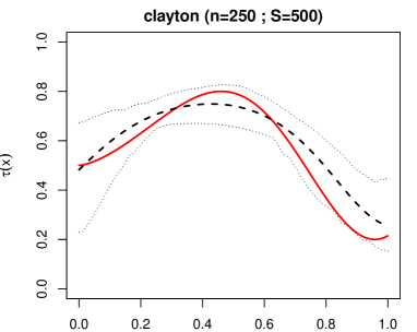
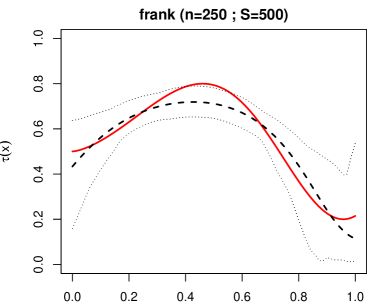
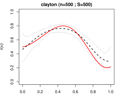
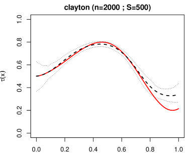
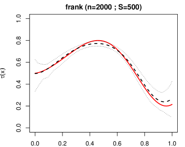
Figure 2: Estimate of the conditional Kendall’s tau corresponding to the additive conditional spline Archimedean copula family fitted to $n$ data generated from a Clayton or a Frank copula with varying Kendall’s tau: true Kendall’s $\tau(x)$ (solid), mean (dashed line) of the $S$ estimated $\tau(x)$ and envelope (dotted lines) containing 95% of the $\tau(x)$ estimates over the $S=500$ replicates.

3.2 The flex-power Archimedean copula family

Other approaches were investigated. One is based on (what we suggest to name) the power Archimedean copula family. It relies on the following result (see e.g. Nelsen, 1999): if $\varphi(\cdot)$ is an Archimedean copula generator, then

1. Interior power transform:
   $\varphi_{\alpha,1}(t)=\varphi(t^{\alpha})$ is also a generator if $\alpha\in(0,1]$ ;

2. Exterior power transform:
   $\varphi_{1,\beta}(t)=\left(\varphi(t)\right)^{\beta}$ is also a generator if $\beta\geq 1$.

The effect of $\alpha$ and $\beta$ on a reference generator $\varphi(t)$ (with Kendall’s tau $\tau_{0}$) is illustrated on Fig. 3 when starting from a Clayton($\theta=1$) generator.

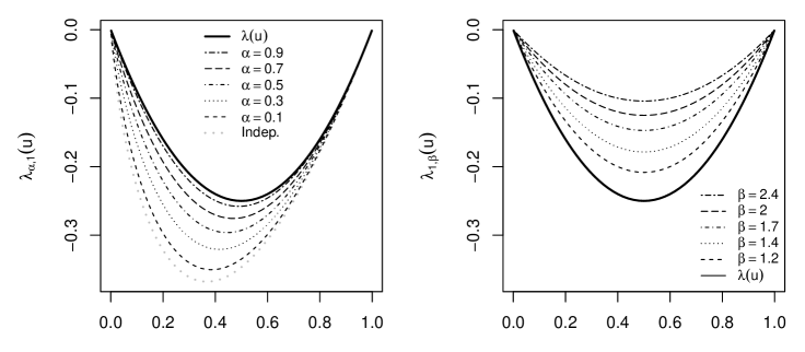
Figure 3: Effect of $\alpha$ and $\beta$ on the lambda function in the power Archimedean family (for a Clayton($\theta=1$) reference generator).

Remembering the relationship between Kendall’s tau and the area decribed by the lambda function and the horizontal axis, see (2.1), one can see that Kendall’s tau increases with $\alpha$ (with a maximal value $\tau_{0}$ when $\alpha=1$, corresponding to the reference generator) and with $\beta$ (with a minimal value $\tau_{0}$ when $\beta=1$).

We suggest to consider both transforms to model changes of the copula generator with covariates, i.e. to take

$$\varphi_{\alpha,\beta}(t|x)=\left[\varphi(t^{\alpha(x)})\right]^{\beta(x)}$$ (3.11)

with flexible forms for

• the reference generator $\varphi(\cdot)$, see (2.3)-(2.4) ;

• the interior power

  $$\alpha=\alpha(x)=\left[1+\left(\sum_{k=1}^{K^{*}}b_{k}^{*}(x)\alpha_{k}\right)^{2}\right]^{-1}~{};$$ (3.12)

• the exterior power

  $$\beta=\beta(x)=1+\left(\sum_{k}^{K^{*}}b_{k}^{*}(x)\beta_{k}\right)^{2},$$ (3.13)

where $\{b_{k}^{*}(\cdot):k=1,\ldots,K^{*}\}$ denotes a cubic B-spline basis on the covariate space (relocated and rescaled to take values in $(0,1)$). That model includes $(K+2K^{*})$ parameters. Like for the reference generator, penalties can be introduced to favor smooth changes with $x$ for $\alpha(x)$ and $\beta(x)$, and, hence, for the conditional copula generator $\varphi_{\alpha,\beta}(t|x)$. If $\kappa_{\alpha}$ (resp. $\kappa_{\beta}$) denote the penalty coefficients for the spline parameters $\bm{\alpha}$ (resp. $\bm{\beta}$) in $\alpha(x)$ (resp. $\beta(x)$) and $P_{\alpha}$ (resp. $P_{\beta}$) the corresponding penalty matrix, then one can show, using gamma priors $\kappa_{\alpha}\sim{\cal G}(a_{\alpha},b_{\alpha})$, $\kappa_{\beta}\sim{\cal G}(a_{\beta},b_{\beta})$ and the same reasoning as in Section 2, that the marginal posterior for the spline coefficients is

$$p(\bm{\theta},\bm{\alpha},\bm{\beta}|{\cal D}) \propto\int_{0}^{+\infty}\int_{0}^{+\infty}\int_{0}^{+\infty}L(\bm{\theta},\bm{\alpha},\bm{\beta}|D)\,p(\bm{\theta}|\kappa)$$

$$\hskip 43.05542pt\,p(\bm{\alpha}|\kappa_{\alpha})\,p(\bm{\beta}|\kappa_{\beta})\,p(\kappa)\,p(\kappa_{\alpha})\,p(\kappa_{\beta})\,d\kappa\,d\kappa_{\alpha}\,d\kappa_{\beta}$$

$$\propto{L(\bm{\theta},\bm{\alpha},\bm{\beta}|{\cal D})\over\left(b+{1\over 2}\bm{\theta}^{\prime}P\bm{\theta}\right)^{a+{\rho(P)\over 2}}\left(b_{\alpha}+{1\over 2}\bm{\alpha}^{\prime}P_{\alpha}\bm{\alpha}\right)^{a_{\alpha}+{\rho(P_{\alpha})\over 2}}\left(b_{\beta}+{1\over 2}\bm{\beta}^{\prime}P_{\beta}\bm{\beta}\right)^{a_{\beta}+{\rho(P_{\beta})\over 2}}}$$ (3.14)

MAP estimates $(\hat{\bm{\theta}},\hat{\bm{\alpha}},\hat{\bm{\beta}})$ for the splines coefficients can be obtained by maximizing the last expression. An adaptive block-Metropolis algorithm can be set up by mimicking the approach in Section 3.1.1 to sample the joint posterior of the spline parameters.

3.2.1 Simulation study

When the data are generated from the power Archimedean family where the interior and exterior powers are functions of a covariate $x$, one can show, using simulations (not reported to save space) that the flex-power family is able to estimate the underlying conditional copula in a precise and nearly unbiased way for large sample sizes. This is not surprising given the results in Section 2.3.

Instead, we report the results obtained when fitting the flex-power Archimedean family to the same datasets as in Section 3.1.2. Given that the data were simulated outside the flex-power family, we did not expect a perfect reconstruction of the underlying dependence structure, but like for the additive model, hoped that reasonable estimations for the changing strength of dependence would be obtained by forcing that model. This is indeed the conclusion that can be drawn by inspecting Fig. 4 where the mean (over the $S$ replicates) of the estimated conditional Kendall’s tau corresponding to the fitted flex-power Archimedean copula can be compared to the function $\tau(x)$ used to simulate the data. Whatever the underlying copula or sample size, the bias for a given $x$ is small and decreases with $n$. A comparison of Figs. 2 and 4 suggests that, in the framework of the simulation study, the flex-power family is a bit more performant than the additive one, at the cost of $K^{*}$ extra (spline) parameter (per covariate).

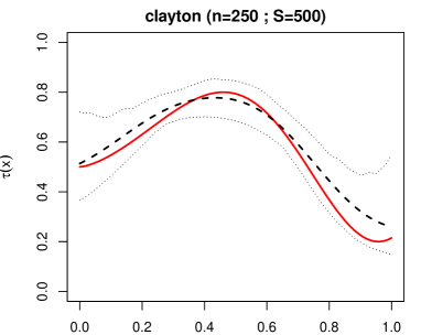
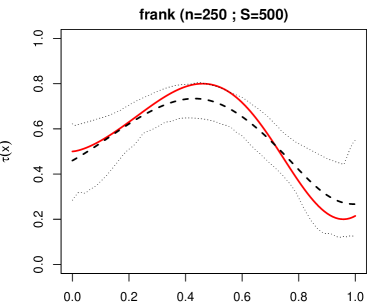
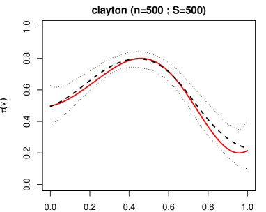
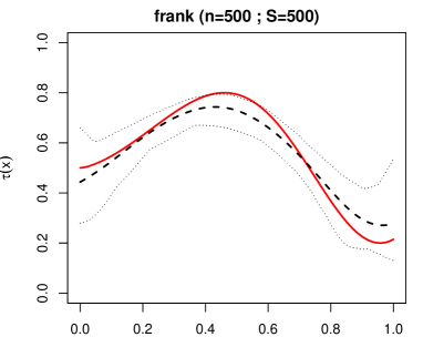
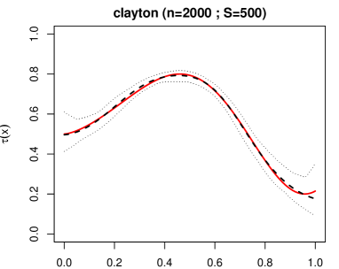
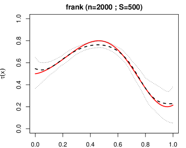
Figure 4: Estimate of the conditional Kendall’s tau corresponding to a flex-power Archimedean copula fitted to $n$ data generated from a Clayton or a Frank copula with varying Kendall’s tau: true Kendall’s $\tau(x)$ (solid), mean (dashed line) of the $S$ estimated $\tau(x)$ and envelope (dotted lines) containing 95% of the $\tau(x)$ estimates over the $S=500$ replicates.

4 Applications

4.1 Growth curves

The additive conditional spline (Model 1) and flex-power (Model 2) Archimedean copula models were also applied on the growth data mentioned in Section 1 (see also Fig. 1). It provides the height ($Y_{1}$) and weight ($Y_{2}$) of $n=441$ young Dutch boys aged between 3 and 21. The margins were first modelled using the nonparametric additive location-scale model described in Lambert (2013),

$$Y_{j}=\mu_{j}(x)+\sigma_{j}(x)\epsilon_{j},$$

where $\mu_{j}(x)$ and $\sigma_{j}(x)$ denotes the conditional median and inter-quartile range of $Y_{j}$ given Age ($=X$). The smooth evolution of these quantities, as well as the pivotal distributions of the $\epsilon_{j}$’s were described using penalized B-splines. The resulting fitted conditional deciles for $Y_{1}$ and $Y_{2}$ are displayed on Fig. 5. It reveals the nonlinear relationship between the responses and Age as well as their increasing dispersion with the latter variate.

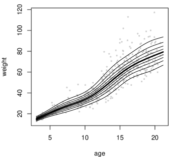
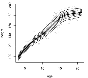
Figure 5: Growth dataset: fitted conditional deciles for Weight and Height given Age using the flexible location-scale model in Lambert (2013).

Copula model	# par.	e.d.	DIC
Model 0 (Unconditional)	11	3.2	-310.4
Model 1 (additive)	16	6.0	-319.0
Model 2 (flex-power)	21	7.0	-318.4

Table 13: Growth dataset: effective number of parameters (e.d.) and DIC in the fitted copula models.

The unconditional and the two conditional copula models were adjusted on the fitted conditional quantiles,

$$\left\{\left(x_{i},\hat{u}_{1|x_{i}}=\hat{F}_{1}(y_{1i}|x_{i}),\hat{u}_{2|x_{i}}=\hat{F}_{2}(y_{2i}|x_{i})\right):i=1,\ldots,n\right\},$$

using the methodology described in Sections 2 (Model 0), 3.1 (Model 1) and 3.2 (Model 2), respectively, with $K=11$, $K^{*}=5$ and $b=b_{\alpha}=b_{\gamma}=b_{\beta}=1$. Therefore, Model 0, Model 1 and Model 2 include $K=11$, $K+K^{*}=16$ and $K+2K^{*}=21$ parameters, respectively (with identifiability constraints). Adaptive block-Metropolis algorithms with chains of length $30,000$ (and a burnin of $1,000$) and initial values set at the MAP estimates were used to explore the joint posterior of the spline parameters in the two models. The deviance information criterions (DIC, Spiegelhalter et al. (2002)) are much smaller in Models 1 & 2 than in Model 0, suggesting a significant change of the strength of association between the two responses with the covariate, see Table 13. Smaller values were obtained for the DIC and for the effective number of parameters in Model 1 (compared to Model 2). The posterior mean of the conditional Kendall’s tau, also estimated from the MCMC chains (see e.g.  (3.10), is plotted with a 95% credible region in Fig. 6. It confirms and quantifies the decreasing association between weight and height suspected from Fig. 1. It is very large at early childhood and decreases afterwards with an apparent acceleration at the start of puberty.

Additive conditional spline model (Model 1)
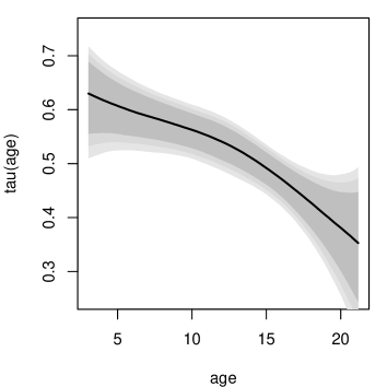
Flex-power model (Model 2)

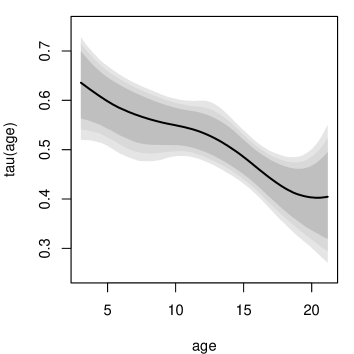
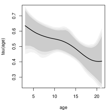
Figure 6: Growth dataset: fitted (solid line) conditional Kendall’s tau under the additive conditional spline and the flex-power Archimedean copula models. Grey areas corresponds to .80, .90 and .95 pointwise (left panel) or simultaneous (right panel) credible regions for $\tau$(age).

The fitted joint distribution can also be visualized for any value of the covariate, see Fig. 7, where its contours for three values of Age are superposed to the scatterplot of the whole dataset.

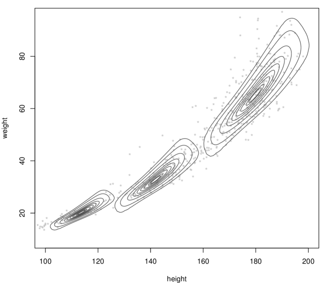
Figure 7: Growth dataset: contours of the fitted joint distribution for Height and Weight at age 5, 10 and 17.

4.2 Blood pressures and cholesterol level

The second example is based on data coming from the Framingham Heart study data (http://www.framingham.com/heart/). We restrict our attention to the evolution with the cholesterol level ($X=\text{CHOL}$) of the association between the diastolic ($Y_{1}=\text{DBP}$) and the systolic ($Y_{2}=\text{SBP}$) blood pressures (in $mmHg$) measured on 663 male subjects at their first visit). The relation between each of the blood pressures with cholesterol was quantified using regression models for the location of a 4-parameter skewed Student distribution (Fernandez and Steel, 1998), see Section 6 in Lambert (2007) for more details, yielding fitted marginal quantiles

$$\left\{\left(x_{i},\hat{u}_{1|x_{i}}=\hat{F}_{1}(y_{1i}|x_{i}),\hat{u}_{2|x_{i}}=\hat{F}_{2}(y_{2i}|x_{i})\right):i=1,\ldots,n\right\}.$$

We first assume that the underlying copula is Archimedean and independent of CHOL: it is specified using the new spline expression proposed in (2.3) with $K=11$ B-splines in the basis and a 3rd order penalty. Figure 8 illustrates the smoothness of the fitted joint distribution (see the improvement over Fig. 5 in Lambert (2007)) and suggests that the Gumbel copula is a good parametric approximation to the dependence structure underlying the log-blood pressures.

Figure 8: Fitted joint distribution for the log-diastolic and log-systolic blood pressures for an average cholesterol level using the flexible spline form (solid contours) or the Gumbel generator (dashed contours).

Conditional copulas were also fitted using the methodology described in Sections 3.1 and 3.2 with the same parameters as in the first application. A comparison of the DIC values for the unconditional copula model and for the conditional ones (see Table 14) suggests that the strength of association between blood pressures is not changing with the cholesterol level.

Copula model	# par.	e.d.	DIC
Model 0 (Unconditional)	11	4.2	-569.0
Model 1 (additive)	16	5.2	-567.9
Model 2 (flex-power)	21	5.1	-567.5

Table 14: Blood pressure dataset: effective number of parameters (e.d.) and DIC in the fitted copula models.

This can be visualized on Fig. 9 where the simultaneous credible regions for the conditional Kendall’s tau in the additive and in the flex-power Archimedean copula families are superposed to the HPD interval $(0.52,0.58)$ for $\tau$ in the unconditional copula model.

Additive conditional spline (Model 1)	Flex-power model (Model 2)

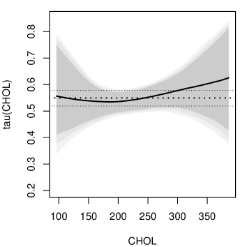
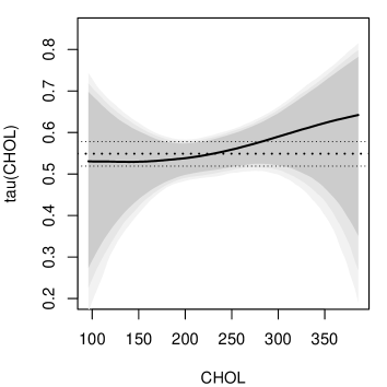
Figure 9: Blood pressure dataset: fitted (solid line) conditional Kendall’s tau under the additive conditional spline and the flex-power Archimedean copula models. Grey areas corresponds to .80, .90 and .95 simultaneous credible regions for $\tau$(CHOL). The point estimate (dashed line) and the HPD region (dotted line) for Kendall’s tau in the unconditional copula model are also provided.

5 Discussion

A performant spline estimator for the generator of an Archimedean copula has been proposed. A large simulation study has shown that it has nearly negligible bias and credible regions with coverage probabilities closed to their nominal values even for moderate sample sizes.

It has been extended to change smoothly with a covariate using either an additive model for the spline coefficients or flexible (spline based) power transforms of the generator and of its argument. Again, simulation studies suggest that these models are quite flexible and useful to describe changes in conditional association structures.

It can be extended to handle multiple categorical or continuous covariates using additive forms such as in (3.7). More than two responses can also be considered using conditional copulas of the form

$$C(u_{1},\ldots,u_{J}|x)=\varphi^{-1}\left({\varphi(u_{1}|x)+\ldots+\varphi(u_{J}|x)}|x\right),$$

but one should question the validity of an exchangeable dependence structure in the specific modelling exercise.

A joint estimation of the parameters involved in the marginal models and in the conditional copula structure is also possible and straightforward to manage in a Bayesian framework. Unless at least one of the margins is discrete, it is not obvious that one would gain anything substantial by merging these modelling efforts in a single inferential procedure.

Besides additive models, an extension to hierarchical settings involving repeated measurements (such as with clustered or longitudinal data) is certainly worth considering, but out of scope for this paper. The proposed conditional copula models can also be used as building block in pair copula constructions such as in regular vines (see e.g. Aas et al., 2009).

Appendix A Likelihood in the spline copula model

From a computational point of view, we found convenient to rewrite the likelihood as

$$L({\bm{\theta}})=-\prod_{i=1}^{n}\left(1-\lambda^{\prime}_{\bm{\theta}}(C_{i})\right){\lambda_{\bm{\theta}}(C_{i})\over\lambda_{\bm{\theta}}(u_{i})\lambda_{\bm{\theta}}(v_{i})}\,{\varphi_{\bm{\theta}}(u_{i})\,\varphi_{\bm{\theta}}(v_{i})\over\left({\varphi_{\bm{\theta}}(u_{i})+\varphi_{\bm{\theta}}(v_{i})}\right)^{2}}$$ (A.1)

where

$$\lambda_{\bm{\theta}}(u)={\varphi_{\bm{\theta}}(u)\over\varphi^{\prime}_{\bm{\theta}}(u)}={-1\over g_{\bm{\theta}}^{\prime}(S(u))S^{\prime}(u)}.$$

The value of $C_{i}$ is given by

$$C_{i}=\varphi_{\bm{\theta}}^{-1}(\varphi_{\bm{\theta}}(u_{i})+\varphi_{\bm{\theta}}(v_{i})).$$

The function $\varphi_{\bm{\theta}}^{-1}(\cdot)$ can be computed numerically using an iterative method. The following algorithm turns to be very efficient. Assume that one looks for $u$ such that $\varphi^{-1}_{\bm{\theta}}(x)=u$. This is equivalent to finding the root of $f(\cdot)$ with $f(u)=g_{\bm{\theta}}(S(u))+\log(x)$. Starting from $u=u^{(0)}$, the guess $u^{(t+1)}$ at iteration $t+1$ (resulting from a Newton step) is such that $S(u^{(t+1)})=S(u^{(t)})+\delta^{(t)}$ with $\delta^{(t)}=-f(u^{(t)})/g^{\prime}(S(u^{(t)}))$. Starting from $C_{i}^{(0)}=u_{i}v_{i}$ and letting $x_{i}=\varphi_{\bm{\theta}}(u_{i})+\varphi_{\bm{\theta}}(v_{i})$, that procedure can be vectorized to compute $C_{i}$ ($i=1,\ldots,n$) with a single loop in three or four iterations. Finally, note that the quantities $\lambda^{\prime}_{\bm{\theta}}(C_{i})$ in the likelihood can be approximated using finite differences of the lambda function.

References

- Aas et al. (2009) Aas, K., Czado, C., Frigessi, A., and Bakken, H. (2009). Pair-copula constructions of multiple dependence. Insurance Mathematics and Economics, 44(2), 182–198.
- Abegaz et al. (2012) Abegaz, F., Gijbels, I., and Veraverbeke, N. (2012). Semiparametric estimation of conditional copulas. Journal of Multivariate Analysis, 110, 43–73.
- Acar and Craiu (2011) Acar, E. and Craiu, R. (2011). Dependence calibration in conditional copulas: A nonparametric approach. Biometrics, 67, 445–453.
- Chen and Shao (1999) Chen, M.-H. and Shao, Q.-M. (1999). Monte Carlo estimation of Bayesian credible and HPD intervals. Journal of the American Statistical Association, 8(1), 69–92.
- Craiu and Sabeti (2012) Craiu, R. and Sabeti, A. (2012). In mixed company: Bayesian inference for conditional copulas models with discrete and continuous outcomes. Journal of Multivariate Analysis, 110, 106–120.
- Eilers and Marx (1996) Eilers, P. H. C. and Marx, B. D. (1996). Flexible smoothing with B-splines and penalties. Statistical Science, 11, 89–121.
- Fernandez and Steel (1998) Fernandez, C. and Steel, M. (1998). On Bayesian modeling of fat tails and skewness. Journal of the American Statistical Association, 93(441), 359–371.
- Genest and MacKay (1986) Genest, C. and MacKay, R. J. (1986). The joy of copulas: Bivariate distributions with uniform marginals. The American Statistician, 40, 280–283.
- Gijbels et al. (2011) Gijbels, I., Veraverbeke, N., and Omelka, M. (2011). Conditional copulas, association measures and their applications. Computational Statistics and Data Analysis, 55, 1919–1932.
- Gijbels et al. (2012) Gijbels, I., Omelka, M., and Veraverbeke, N. (2012). Multivariate and functional covariates and conditional copulas. Electronic Journal of Statistics, 6, 1273–1306.
- Haario et al. (2001) Haario, H., Saksman, E., and Tamminen, J. (2001). An adaptive Metropolis algorithm. Bernoulli, 7, 223–242.
- Hafner and Reznikova (2010) Hafner, C. M. and Reznikova, O. (2010). Efficient estimation of a semiparametric dynamic copula model. Computational Statistics and Data Analysis, 54(11), 2609–2627.
- Held (2004) Held, L. (2004). Simultaneous posterior probability statements from Monte Carlo output. Journal of Computational and Graphical Statistics, 13, 20–35.
- Jullion and Lambert (2007) Jullion, A. and Lambert, P. (2007). Robust specification of the roughness penalty prior distribution in spatially adaptive Bayesian P-splines models. Computational Statistics and Data Analysis, 51(5), 2542–2558.
- Lambert (2007) Lambert, P. (2007). Archimedean copula estimation using Bayesian splines smoothing techniques. Computational Statistics and Data Analysis, 51(12), 6307–6320.
- Lambert (2013) Lambert, P. (2013). Nonparametric additive location-scale models for interval censored data. Statistics and Computing, 23, 75–90.
- Lambert and Vandenhende (2002) Lambert, P. and Vandenhende, F. (2002). A copula based model for multivariate non normal longitudinal data: analysis of a dose titration safety study on a new antidepressant. Statistics in Medicine, 21, 3197–3217.
- Lang and Brezger (2004) Lang, S. and Brezger, A. (2004). Bayesian P-splines. Journal of Computational and Graphical Statistics, 13, 183–212.
- Nelsen (1999) Nelsen, R. B. (1999). An Introduction to Copulas. Springer-Verlag.
- Patton (2006) Patton, A. (2006). Modelling asymmetric exchange rate dependence. International Economic Review, 47(2), 527–556.
- Sklar (1959) Sklar, A. (1959). Fonctions de répartition à dimensions et leurs marges. Publ. Inst. Statist. Univ. Paris, 8, 229–231.
- Spiegelhalter et al. (2002) Spiegelhalter, D., Best, N., Carlin, B., and van der Linde, A. (2002). Bayesian measures of model complexity and fit. Journal of the Royal Statistical Society, Series B, 64, 583–639.
- Vandenhende and Lambert (2005) Vandenhende, F. and Lambert, P. (2005). Local dependence estimation using semiparametric Archimedean copulas. The Canadian Journal of Statistics, 33, 377–388.
- Veraverbeke et al. (2011) Veraverbeke, N., Omelka, M., and Gijbels, I. (2011). Estimation of a conditional copula and association measures. Scandinavian Journal of Statistics, 38, 766–780.