Sampling Content Distributed Over Graphs

Abstract

Despite recent effort to estimate topology characteristics of large graphs (i.e., online social networks and peer-to-peer networks), little attention has been given to develop a formal methodology to characterize the vast amount of content distributed over these networks. Due to the large scale nature of these networks, exhaustive enumeration of this content is computationally prohibitive. In this paper, we show how one can obtain content properties by sampling only a small fraction of vertices. We first show that when sampling is naively applied, this can produce a huge bias in content statistics (i.e., average number of content duplications). To remove this bias, one may use maximum likelihood estimation to estimate content characteristics. However our experimental results show that one needs to sample most vertices in the graph to obtain accurate statistics using such a method. To address this challenge, we propose two efficient estimators: special copy estimator (SCE) and weighted copy estimator (WCE) to measure content characteristics using available information in sampled contents. SCE uses the special content copy indicator to compute the estimate, while WCE derives the estimate based on meta-information in sampled vertices. We perform experiments to show WCE and SCE are cost effective and also “asymptotically unbiased”. Our methodology provides a new tool for researchers to efficiently query content distributed in large scale networks.

1 Introduction

Nowadays online social networks (OSNs) (i.e., Facebook and Twitter) and P2P networks (i.e., BitTorrent) are two popular classes of Internet applications. Measuring content characteristics such as file duplication level and information spreading rate on such networks become important since it helps one develop effective advertising strategies [1], and provides valuable information for designing content delivery strategies, i.e., video sharing techniques [2] to increase video pre-fetch accuracy by delivering videos based on users’ social relationships and interests, or to develop information seeding techniques [3] to minimize the peak load of cellular networks by proactively pushing some videos to OSN users. Meanwhile measuring characteristics of OSNs’ content provided by other networks also helps to us understand interactions between different networks, i.e., [2] found that 80% of videos in Facebook come from other video service providers such as YouTube.

Due to the large sizes of these networks, it is a challenge to measure content properties, such as the distribution of tweets in an OSN by the number of replies/retweets, or the distribution of videos in OSNs by external video service providers. To measure content properties, we formulate the problem as follows. Define $L(\mathbf{c})$ as a generic labeling function of content $\mathbf{c}$, with range $\mbox{\boldmath$L$}=\{l_{0},...,l_{K}\}$. We present methods to estimate the content distribution $\mbox{\boldmath$\omega$}=(\omega_{0},\ldots,\omega_{K})$, where $\omega_{k}$ ($0\leq k\leq K$) is the fraction of content with label $l_{k}$. For example, $L(\mathbf{c})$ can be defined as the number of comments of post $\mathbf{c}$ in OSNs, and then $\omega_{k}$ is the fraction of posts with $k$ comments, where $\mbox{\boldmath$L$}=\{0,1,2,\ldots\}$. In P2P networks, $L(\mathbf{c})$ can denote the number of replicas of file $\mathbf{c}$; then $\omega_{k}$ is the fraction of files possessing $k$ replicas, where $\mbox{\boldmath$L$}=\{1,2,\ldots\}$. Similarly $L(\mathbf{c})$ can also be the file type of $c$ in P2P networks, with $\mbox{\boldmath$L$}=\{l_{0}\!=\!``video",l_{1}\!=\!``musci",l_{2}\!=\!``text",l_{3}\!=\!``others"\}$. Then $\omega_{k}$ ($k=0,1,2,3$) is the fraction of files of type $l_{k}$.

Figure 1: An example of sampling files in a P2P network.

Due to the size of these networks, the direct enumeration is computationally prohibitive and one must consider using sampling methods to estimate $\omega$. Unfortunately, previous graph sampling work developed for estimating degree or workplace distributions [4, 5] does not directly apply in our context. This is because content and vertex are intrinsically different since content may be duplicated. To illustrate this, consider a simple example of a P2P network as shown in Fig. 1. Assume file $F_{1}$ is cached by $10,000$ users, $F_{2}$ is cached by two users $u$ and $v$, and $F_{3}$ is cached by user $u$. When sampling is applied, clearly $F_{1}$ is more likely to be observed than $F_{2}$ and $F_{3}$. Therefore, estimation algorithms for topological metrics such as degree distribution cannot be blindly applied. They need to be modified to deal with biases introduced because of the nature of content characterization.

To the best of our knowledge, our work is the first analytical and qualitative study on the problem of estimating characteristics of content distributed over large graphs. We propose methods to accurately estimate the content distribution $\omega$. Our contributions are:
$\bullet$ We show that when sampling is naively applied, there can be huge bias in content statistics $\omega$. One can remove this bias using the maximum likelihood estimation. However our experimental results show that one needs to sample most vertices in the graph in order to obtain accurate statistics.

$\bullet$ We present two efficient methods to estimate the content distribution $\omega$ using available information in sampled content based on two different assumptions. The first method assumes that we can determine whether a collected content copy is a source or not, which is true for most OSNs that have a label in each content copy to indicate whether it is a source or a duplicated copy. For example, a tweet in microblog networks can be classified as an original tweet or a retweet. Therefore, one can utilize a special content copy set consisting of all original tweets to characterize distribution of tweets in the network. To measure $\omega$ of content in these networks, we propose a special copy estimator (SCE) based on collected source content copies. We will show that SCE uses only a fraction of sampled content copies. Moreover for networks such as P2P networks that cannot classify video copies as original and not original, we propose another weighted copy estimator (WCE). It assumes that each content copy records the number of copies its content holds. This feature is true for many OSNs [6, 7, 8] and P2P networks [9]. Our experiments show that WCE and SCE are asymptotically unbiased, and WCE is much more accurate estimator than SCE.

$\bullet$ We also use WCE to estimate graph structure statistics for OSNs such as Sina microblog [7] and Xiami [8] where users maintain graph property summaries of their neighbors. For example, by crawling the profile of a user in Sina microblog, we can obtain its neighbors’ properties such as the number of followers, the number of following, the number of tweets, etc. This allows us to collect more information than previous graph sampling methods under the same sampling cost. Since a user’s graph property summary can be viewed as content maintained by itself and its neighbors, we apply WCE to estimate graph statistics. Our experiments show that WCE can obtain the same level of accuracy of graph properties with a much less sampling cost as compared with previous works.

This paper is organized as follows. In Section 2 we summarize the most popular graph sampling techniques. Section 3 presents several new methods for measuring characteristics of content in the graph. The performance evaluation and testing results are presented in Section 4. Section 5 presents real applications on Twitter and Sina microblog websites. Related work is given in Section 6, and conclusion is given in Section 7.

2 Graph Sampling Methods

In this section we present some graph sampling methods that are underlying techniques for sampling content discussed in the later Section. For ease of presentation, we assume the underlying graph is undirected. One way to convert a directed graph into an undirected graph is by ignoring the direction of edges. Consider an undirected graph $G=(V,E)$, where $V$ is the set of vertices and $E$ is the set of undirected edges. Breadth-First-Search (BFS) is one of most popular graph sampling techniques. However it introduces a large bias towards high-degree vertices that is unknown and difficult to remove in general graphs [10, 11]. Therefore we do not consider BFS in this paper. In what follows, we present popular graph sampling methods: Uniform Vertex Sampling (UNI) and Random Walk (RW), Metropolis-Hasting RW (MHRW) [12], and Frontier Sampling (FS) [5]. Unless we state otherwise, we denote $\mbox{\boldmath$\pi$}=(\pi_{v}\!:\!v\in V)$ as the probability distribution for the underlying sampling method, where $\pi_{v}$ is the probability that vertex $v$ is sampled at each sampling step.

2.1 Uniform Vertex Sampling (UNI)

UNI randomly samples vertices from the vertex set $V$ uniformly and independently with replacement. Not all network graphs support UNI but some do. For example, one can view Wikipedia as a graph and Wikipedia provides a query API to obtain a randomly sampled vertex (wiki page) from its entire vertices. Therefore, at each step, UNI samples each vertex $v$ with the same probability, so we have

$$\pi_{v}^{\text{UNI}}=\frac{1}{|V|},\quad v\in V.$$

For networks such as Facebook, MySpace, Flickr [13], Renren, Sina microblog, and Xiami, one can sample users (vertices) as users have numeric IDs between the minimum and the maximum ID values. Unfortunately, ID values of users in many networks (e.g. Flickr, Facebook, Sina microblog, and MySpace) are not sequentially assigned, and the ID space is sparsely populated [14, 15]. Hence, a randomly generated ID may not correspond to a valid user, so considerable computational effort in generating a random ID will be wasted. Therefore, UNI should only be applied to those graphs whose user ID values are densely packed.

2.2 Random Walk (RW)

RW has been extensively studied in the graph theory literature [16]. From an initial vertex, a walker selects a neighbor at random as the next-hop vertex. The walker moves to this neighbor and repeats the process. Denote $\mathcal{N}(u)$ as the set of neighbors of any vertex $u$, $\text{deg}(u)=|\mathcal{N}(u)|$ is the degree of $u$. Formally, RW can be viewed as a Markov chain with transition matrix $P^{\text{RW}}=[P^{\text{RW}}_{u,v}]$, $u,v\in V$, where $P^{\text{RW}}_{u,v}$ is defined as the probability of vertex $v$ being selected as the next-hop vertex given that its current vertex is $u$, we have:

$$P^{\text{RW}}_{u,v}=\left\{\begin{array}[]{ll}\frac{1}{\text{deg}(u)}&\text{if }v\in\mathcal{N}(u),\\ 0&\text{otherwise.}\end{array}\right.$$

The stationary distribution $\mbox{\boldmath$\pi$}^{\text{RW}}$ of this Markov chain is

$$\pi_{v}^{\text{RW}}=\frac{\text{deg}(v)}{2|E|},\quad v\in V.$$

For a connected and non-bipartite graph $G$, the probability of being at a vertex $v\in V$ converges to the above stationary distribution [16]. Note that $\mbox{\boldmath$\pi$}^{\text{RW}}$ is biased toward vertices with high degree. However, this bias can be corrected [17, 18].

2.3 Metropolis-Hastings Random Walk (MHRW)

MHRW [19, 12, 4] provides another way to modifies RW using Metropolis-Hasting technique [20, 21, 22], which aims to collect vertices uniformly. To generate a sequence of random samples from a desired stationary distribution $\pi^{\text{MHRW}}$, the Metropolis-Hastings technique is a Markov chain Monte Carlo method based on modifying the transition matrix of RW as

$$P_{u,v}^{\text{MHRW}}=\left\{\begin{array}[]{ll}P^{\text{RW}}_{u,v}\min\left(\frac{\pi^{\text{MHRW}}_{v}P^{\text{RW}}_{v,u}}{\pi^{\text{MHRW}}_{u}P^{\text{RW}}_{u,v}},1\right)&\text{if }v\in\mathcal{N}(u),\\ 1-\sum_{w\neq u}P_{u,w}^{MHRW}&\text{if }v=u,\\ 0&\text{otherwise}.\end{array}\right.$$

For a MHRW with target distribution $\pi^{\text{MHRW}}=\pi^{\text{UNI}}$, it works as follows: At each step, MHRW selects a neighbor $v$ of current vertex $u$ at random and then accept the move randomly with probability $\min\left(\frac{\text{deg}(u)}{\text{deg}(v)},1\right)$. Otherwise, MHRW still remains at $u$. Essentially, MHRW removes the bias of RW at each step by rejecting moves towards high degree vertices with a certain probability.

2.4 Frontier Sampling (FS)

FS [5] is a centrally coordinated sampling which performs $T$ dependent RWs in graph $G$. Compared to a single RW, FS is less likely to get stuck in a loosely connected component of $G$. Denote $\vec{L}=(v_{1},\ldots,v_{T})$ as the vector with $T$ vertices. Each $v_{i}$ ($1\leq i\leq T$) is initialized with a random vertex uniformly selected from $V$. At each step, FS selects a vertex $u\in\vec{L}$ with probability $\frac{\text{deg}(u)}{\sum_{\forall v\in\vec{L}}\text{deg}(v)}$, and uniformly selects a node $w$ from $\mathcal{N}(u)$, the neighbors of $u$. Thus $w$ is uniformly selected from the vertices connected to the vertices in $\vec{L}=(v_{1},\ldots,v_{T})$. Then FS replaces $u$ by $w$ in $\vec{L}$ and add $w$ to sequence of sampled vertices. If $G$ is a connected and non-bipartite graph, the probability that a vertex $v$ is sampled by FS converges to the following distribution

$$\pi_{v}^{\text{FS}}=\frac{\text{deg}(v)}{2|E|},\quad v\in V.$$

2.5 Estimator

Previous work has considered how to estimate topology properties, e.g., degree distribution, via sampling methods. Define $L^{\prime}(v)$ to be the vertex label of vertex $v$ under study, with range $\mbox{\boldmath$L^{\prime}$}=\{l_{0}^{\prime},...,l_{K^{\prime}}^{\prime}\}$. Denote vertex label density $\mbox{\boldmath$\tau$}=(\tau_{0},\ldots,\tau_{K^{\prime}})$, where $\tau_{k}$ ($0\leq k\leq K^{\prime}$) is the fraction of vertices with label $l_{k}^{\prime}$. For example, when $L^{\prime}(v)$ is defined as the degree of vertex $v$, and $\tau$ is the degree distribution. To estimate $\tau$, the stationary distribution $\pi$ is needed to correct the bias induced by the underlying sampling method. Since the values of $|V|$ and $|E|$ are usually unknown, unbiasing the error is not straightforward. Instead, one may use a non-normalized stationary distribution $\hat{}\mbox{\boldmath$\pi$}=(\hat{\pi}_{v}:v\in V)$ to reweight sampled vertices $s_{i}$ ($1\leq i\leq n$), where $\hat{\pi}_{v}$ is computed as

$$\hat{\pi}_{v}=\left\{\begin{array}[]{ll}1&\text{for UNI and MHRW},\\ \text{deg}(v)&\text{for RW and FS}.\\ \end{array}\right.$$ (1)

Let $\mathbf{1}(\mathbf{P})$ define the indicator function that equals one when predicate $\mathbf{P}$ is true, and zero otherwise. Finally $\tau_{k}$ is estimated as follows

$$\hat{\tau}_{k}=\frac{1}{S}\sum_{i=1}^{n}\frac{\mathbf{1}(L^{\prime}(s_{i})=l_{k}^{\prime})}{\hat{\pi}_{s_{i}}},\quad 0\leq k\leq K^{\prime},$$

where $S=\sum_{i=1}^{n}{\hat{\pi}}_{s_{i}}^{-1}$.

In summary, RW and FS are biased to sample vertices with high degree vertices. These biases can be later corrected, giving us smaller estimation errors for the characteristics of high degree vertices. The accuracy of RW and MHRW is compared in [23, 4]. RW is shown to be consistently more accurate than MHRW. Compared with RW and MHRW, FS requires UNI sampling for its initial settings, but is more accurate for sampling loosely connected and disconnect graphs [5].

3 Content Sampling Methods

Denote by $\mathbf{C}=\{\mathbf{c}_{1},\ldots,\mathbf{c}_{H}\}$ the set of all content under study, where $H$ is total number of distinct contents in $G$. In this section, we study how to characterize the content distribution $\mbox{\boldmath$\omega$}=(\omega_{0},\ldots,\omega_{K})$ defined in Section 1, that is

$$\omega_{k}=\frac{\sum_{\mathbf{c}\in\mathbf{C}}\mathbf{1}(L(\mathbf{c})=l_{k})}{H},\quad k=0,\ldots,K,$$

where $L(\mathbf{c})$ is the label of content $\mathbf{c}$ with range $\{l_{0},...,l_{K}\}$. We let $c^{*}$ denote a special copy, such as the original source of content $\mathbf{c}$. Note that each content $\mathbf{c}$ has one and only one special copy $c^{*}$. For content $\mathbf{c}\!\in\!\mathbf{C}$, let $\{c^{(1)},\ldots,c^{(f(\mathbf{c}))}\}$ denote the set of its copies appearing in graph $G$ including its special copy $c^{*}$, where $f(\mathbf{c})$ is the number of copies of $\mathbf{c}$. For a content copy $c$, let $v(c)$ be the vertex that maintains $c$. Unless we state otherwise, in what follows the notation $\mathbf{c}$ is used to depict content and $c$ is used to depict a copy of content $\mathbf{c}$. Meanwhile, we define $L(c)=L(\mathbf{c})$ and $f(c)=f(\mathbf{c})$. Let $C_{\mathbf{S}}=\{c_{1}^{*},\ldots,c_{H}^{*}\}$ be a special content copy set. For some graphs, sampling methods can check whether a sampled content copy is special or not and generate such a set $C_{\mathbf{S}}$. For example, a tweet in the Sina microblog can be classified into an original tweet or a retweet, therefore we can generate $C_{\mathbf{S}}$ consisting of all original tweets.

We assume that $n$ vertices $s_{i}$ ($1\leq i\leq n$) are obtained by a graph sampling method that samples a vertex randomly from $V$ according to probability distribution $\pi$ at each sampling step. Denote by $C(s_{i})$ the set of the content copies maintained by vertex $s_{i}$. Denote by $\mathbf{C_{D}}$ the set of content that has at least one copy maintained by sampled vertices $s_{i}$ ($1\leq i\leq n$). In this section, we study how to characterize the content distribution $\omega$ based on $C(s_{i})$, $1\leq i\leq n$.

We present four estimators: (1) distinct content estimator (DCE), (2) maximum likelihood estimator (MLE), (3) special copy estimator (SCE), and (4) weighted copy estimator (WCE). DCE estimates $\omega$ directly based on the collected content $\mathbf{C_{D}}$. Later we will show that content in $\mathbf{C_{D}}$ is not uniformly sampled from $\mathbf{C}$. Therefore estimates of $\omega$ obtained by DCE are biased. MLE uses duplication level information of copies in $C(s_{i})$ ($1\leq i\leq n$) to remove the bias of DCE. However, we will show via experiment that MLE needs to sample most vertices in graph $G$ in order to obtain accurate statistics. SCE and WCE use meta information in sampled content copies to remove sampling biases for estimating $\omega$. SCE estimates $\omega$ based on collected content copies in $C_{\mathbf{S}}$, which assumes that we can determine whether a collected content copy is special or not. WCE utilizes all collected content to estimate $\omega$ based on the assumption that each copy of any content $\mathbf{c}$ records the value of $f(\mathbf{c})$. A list of notations used is shown in Table I.

TABLE I: Table of notations

$s_{i},1\leq i\leq n$	sampled vertices
$\mbox{\boldmath$\pi$}=(\pi_{v}:v\in V)$	vertex sampling probability distribution
$\mathbf{C}=\{\mathbf{c}_{1},\ldots,\mathbf{c}_{H}\}$	set of all content appearing in graph $G$
$L(\mathbf{c})$	label of content $\mathbf{c}\in\mathbf{C}$
$\{l_{0},...,l_{K}\}$	range of label function $L(\mathbf{c})$
$\mbox{\boldmath$\omega$}=(\omega_{0},\ldots,\omega_{K})$	distribution of content by
	the content label
$f(\mathbf{c})$	number of copies that content $\mathbf{c}$
	possesses
$\{c^{(1)},\ldots,c^{(f(\mathbf{c}))}\}$	all copies of content $\mathbf{c}$
$c^{*}$	the special copy of content $\mathbf{c}$
$C_{\mathbf{S}}=\{c_{1}^{*},\ldots,c_{H}^{*}\}$	special content copy set
$c$	a copy of content $\mathbf{c}$
$v(c)$	vertex that maintains content copy $c$
$L(c)$, $f(c)$	$L(c)=L(\mathbf{c})$, $f(c)=f(\mathbf{c})$
$C(v),v\in V$	content copies maintained by vertex $v$
$\mathbf{C_{D}}$	set of content that has a copy
	maintained by sampled vertices $s_{i}$

3.1 Distinct Content Estimator (DCE)

DCE directly estimates $\omega$ using all distinct collected content $\mathbf{C_{D}}$ as follows

$$\hat{\omega}_{k}^{\text{DCE}}=\frac{1}{|\mathbf{C_{D}}|}\sum_{\mathbf{c}\in\mathbf{C_{D}}}\mathbf{1}(L(\mathbf{c})=l_{k}),\quad 0\leq k\leq K.$$

Content $\mathbf{c}\in\mathbf{C}$ is maintained by vertices $v(c^{(j)})$ ($1\leq j\leq f(\mathbf{c})$) and vertex $v(c^{(j)})$ is sampled with probability $\pi_{v(c^{(j)})}$ at each sampling step, therefore the probability that one copy of content $\mathbf{c}$ is collected by randomly sampling a vertex is $\sum_{j=0}^{f(\mathbf{c})}\pi_{v(c^{(j)})}$. Note that this probability depends both on the graph sampling method and the number of copies of $\mathbf{c}$, therefore content in $\mathbf{C_{D}}$ is not uniformly sampled from $\mathbf{C}$. Even when the UNI sampling method is used, where each vertex $u$ is sampled with the same probability $\pi_{u}=\frac{1}{|V|}$, the probability that $\mathbf{C_{D}}$ contains $\mathbf{c}$ is proportional to $\frac{f(\mathbf{c})}{|V|}$. This clearly shows that $\hat{\omega}_{k}^{\text{DCE}}$ using UNI is still biased.

3.2 Maximum Likelihood Estimator (MLE)

In what follows, we use the maximum likelihood estimation method to remove the bias of DCE. Due to page limit, We only present the MLE for graph sampling method UNI with $\pi_{v}=\frac{1}{|V|}$, $v\in V$. Suppose that the graph size is known (this can be estimated by sampling methods proposed in [24]), $n<|V|$ vertices are sampled, and then each copy of $\mathbf{c}$ is sampled with the same probability $p=\frac{n}{|V|}$. For simplicity, we assume that content are distributed over networks uniformly at random. Let $M$ be the maximum number of copies that content has. Denote $P_{i,j}$ as the probability that $i$ copies are sampled for content which has $j$ copies, where $1\leq i\leq j\leq M$. Let $q=1-p$, we have $P_{i,j}=\frac{\binom{j}{i}p^{i}q^{j-i}}{1-q^{j}}$.

When the content label under study is the number of copies associated with content. For randomly sampled content, let $\alpha_{i}$ ($1\leq i\leq M$) be the probability that it has $i$ copies sampled. Note that $\alpha_{i}$ can be estimated based on collected content copies. In what follows, we propose a method to estimate $\omega$ based on the relationship of $\alpha_{i}$ and $\omega$. the likelihood function of $\alpha_{i}$ is

$$\mathcal{L}(\alpha_{i}|\mbox{\boldmath$\omega$})=\sum_{j=i}^{M}\omega_{j}P_{i,j}.$$ (2)

This is similar to packet sampling based flow size distribution estimation studied in [25], where each packet is sampled with probability $p$. Here a flow refers to a group of packets with the same source and destination, and the flow size is the number of packets that it contains. In our context content corresponds to a flow, and its copies to packets in the flow. Therefore we can develop a maximum likelihood estimate $\hat{\omega}_{k}^{\text{MLE}}$ of $\omega_{k}$ ($1\leq k\leq M$) similar to the method proposed in [25].

When the content label under study is insensitive to the number of duplicates. We use the following approach to derive the MLE. Meanwhile it is available in each content copy, which is not a latent property such as the number of copies content has. Define $\beta_{k,j}$ ($0\leq k\leq K$, $1\leq j\leq M$) as the fraction of the number of content with label $l_{k}$ and $j$ copies over the number of content with label $l_{k}$. For randomly sampled content, let $\alpha_{k,i}$ ($1\leq i\leq M$) be the probability that its content label is $l_{k}$ and has $i$ copies sampled. Then the likelihood function of $\alpha_{k,i}$ is

$$\mathcal{L}(\alpha_{k,i}|\mbox{\boldmath$\omega$})=\sum_{j=i}^{M}\beta_{k,j}P_{i,j}.$$

$\alpha_{k,i}$ can be estimated based on collected content copies. Then similar to (2), we can develop a maximum likelihood estimate $\hat{\beta}_{k,j}$ of $\beta_{k,j}$, $1\leq j\leq M$. Since

$$\alpha_{k}=\omega_{k}\sum_{i=1}^{M}\sum_{j=i}^{M}\beta_{k,j}P_{i,j},$$

Then we have the following estimator of $\omega_{k}$

$$\hat{\omega}_{k}^{\text{MLE}}=\frac{\hat{\alpha}_{k}}{S^{\text{MLE}}\sum_{i=1}^{M}\sum_{j=i}^{M}\hat{\beta}_{k,j}P_{i,j}},\quad 0\leq k\leq K,$$

where $\hat{\alpha}_{k}$ is the fraction of sampled content with label $k$, and $S^{\text{MLE}}=\sum_{k=0}^{K}\frac{\hat{\alpha}_{k}}{\sum_{i=1}^{M}\sum_{j=i}^{M}\hat{\beta}_{k,j}P_{i,j}}$. In a later section, we will show that to calculate $\hat{\omega}_{k}^{\text{MLE}}$, one has to sample a large number of vertices in $G$. It is consistent with results observed in [26].

3.3 Special Copy Estimator (SCE)

SCE estimates $\omega$ only using collected special content copies, which are content copies in set $C_{\mathbf{S}}$. For content $\mathbf{c}$, $v(c^{*})$ is the vertex maintained its special copy $c^{*}$. Then the probability that $c^{*}$ is collected by sampling a random vertex is $\pi_{v(c^{*})}$. Similar to the estimator given in Section 2, we use $\hat{}\mbox{\boldmath$\pi$}$ defined in Eq. (1) to estimate $\omega_{k}$ ($0\leq k\leq K$),

$$\hat{\omega}_{k}^{\text{SCE}}=\frac{1}{S^{\text{SCE}}}\sum_{i=1}^{n}\sum_{c\in C(s_{i})}\frac{\mathbf{1}(L(c)=l_{k})\mathbf{1}(c\in C_{\mathbf{S}})}{\hat{\pi}_{s_{i}}},$$ (3)

where $S^{\text{SCE}}=\sum_{i=1}^{n}\sum_{c\in C(s_{i})}\frac{\mathbf{1}(c\in C_{\mathbf{S}})}{\hat{\pi}_{s_{i}}}$. It is important to point out that $\hat{\omega}_{k}^{\text{SCE}}$ is an asymptotically unbiased estimator of $\omega_{k}$. For each vertex $v\in V$, Eq. (1) shows that $\pi_{v}/\hat{\pi}_{v}$ has the same value, denoted as $S_{\pi}$. We have the following equation for each $k=0,\ldots,K$ and $i=1,\ldots,n$

$$\begin{split}&\text{E}\left[\sum_{c\in C(s_{i})}\frac{\mathbf{1}(L(c)=l_{k})\mathbf{1}(c\in C_{\mathbf{S}})}{\hat{\pi}_{s_{i}}}\right]\\ &=\sum_{v\in V}\pi_{v}\sum_{c\in C(v)}\frac{\mathbf{1}(L(c)=l_{k})\mathbf{1}(c\in C_{\mathbf{S}})}{\hat{\pi}_{v}}\\ &=S_{\pi}\sum_{v\in V}\sum_{c\in C(v)}\mathbf{1}(L(c)=l_{k})\mathbf{1}(c\in C_{\mathbf{S}})\\ &=S_{\pi}\sum_{c\in C_{\mathbf{S}}}\mathbf{1}(L(c)=l_{k})=S_{\pi}H\omega_{k}.\end{split}$$

Applying the law of large numbers, we have

$$\lim_{n\rightarrow\infty}\frac{1}{n}\sum_{i=1}^{n}\sum_{c\in C(s_{i})}\!\!\!\frac{\mathbf{1}(L(c)=l_{k})\mathbf{1}(c\in C_{\mathbf{S}})}{\hat{\pi}_{s_{i}}}\,\,\xrightarrow{a.s.}\,\,S_{\pi}H\omega_{k},$$

where “$a.s.$” denotes “almost sure” converge, i.e., the event happens with probability one. Similarly, we have $\lim_{n\rightarrow\infty}\frac{S^{\text{SCE}}}{n}\xrightarrow{a.s.}S_{\pi}H$. Therefore $\hat{\omega}_{k}^{\text{SCE}}$ is an asymptotically unbiased estimator of $\omega_{k}$.

3.4 Weighted Copy Estimator (WCE)

WCE estimates $\omega$ using all collected content copies $C(s_{i})$ ($1\leq i\leq n$). This estimator is useful for networks (i.e., Sina microblog or Renren) in which each copy of any content $\mathbf{c}$ records the value of $f(\mathbf{c})$, the number of copies $\mathbf{c}$ has in the network. For content $\mathbf{c}$, vertex $v(c^{(j)})$ maintains the copy $c^{(j)}$ ($1\leq j\leq f(\mathbf{c})$), and the vertex is sampled with probability $\pi_{v(c^{(j)})}$. Meanwhile a random vertex maintains a copy of $\mathbf{c}$ with probability proportional to $f(\mathbf{c})$. Therefore we assign a weight $\frac{1}{\hat{\pi}_{v(c^{(j)})}f(\mathbf{c})}$ for $c^{(j)}$ to remove the sampling bias. Finally $\omega_{k}$ ($0\leq k\leq K$) is estimated as follows

$$\hat{\omega}_{k}^{\text{WCE}}=\frac{1}{S^{\text{WCE}}}\sum_{i=1}^{n}\sum_{c\in C(s_{i})}\frac{\mathbf{1}(L(c)=l_{k})}{\hat{\pi}_{s_{i}}f(c)},$$ (4)

where $S^{\text{WCE}}=\sum_{i=1}^{n}\sum_{c\in C(s_{i})}\frac{1}{\hat{\pi}_{s_{i}}f(c)}$. Note that $\hat{\omega}_{k}^{\text{WCE}}$ is an asymptotically unbiased estimator of $\omega_{k}$. To see that, we have the following equation for each $k=0,\ldots,K$ and $i=1,\ldots,n$

$$\begin{split}&\text{E}\left[\sum_{c\in C(s_{i})}\frac{\mathbf{1}(L(c)=l_{k})}{\hat{\pi}_{s_{i}}f(c)}\right]\\ &=\sum_{v\in V}\pi_{v}\sum_{c\in C(v)}\frac{\mathbf{1}(L(c)=l_{k})}{\hat{\pi}_{v}f(c)}\\ &=S_{\pi}\sum_{v\in V}\sum_{c\in C(v)}\frac{\mathbf{1}(L(c)=l_{k})}{f(c)}\\ &=S_{\pi}\sum_{\mathbf{c}\in\mathbf{C}}\sum_{j=1}^{f(\mathbf{c})}\frac{\mathbf{1}(L(c^{(j)})=l_{k})}{f(c^{(j)})}\\ &=S_{\pi}\sum_{\mathbf{c}\in\mathbf{C}}\mathbf{1}(L(\mathbf{c})=l_{k})=S_{\pi}H\omega_{k}.\end{split}$$

Then we have

$$\lim_{n\rightarrow\infty}\frac{1}{n}\sum_{i=1}^{n}\sum_{c\in C(s_{i})}\frac{\mathbf{1}(L(c)=l_{k})}{\hat{\pi}_{s_{i}}f(c)}\xrightarrow{a.s.}S_{\pi}H\omega_{k}.$$

Similarly, we have $\lim_{n\rightarrow\infty}\frac{S^{\text{WCE}}}{n}\xrightarrow{a.s.}S_{\pi}H$. Therefore $\hat{\omega}_{k}^{\text{WCE}}$ is an asymptotically unbiased estimator of $\omega_{k}$.

We also note that, compared with previous sampling methods[5, 4], WCE is a more cost effective method to estimate graph structure statistics for OSNs (i.e., Sina Microblog and Xiami) which carry such meta information. As shown in Fig. 2, the webpage of a user in Sina Microblog maintains a summary for each of its neighbors (both followers and following), which includes graph properties such as the number of followers, the number of following, and the number of posts. Hence, one can obtain properties of any vertex $v$ and all its neighbors by simply sampling $v$. So compared with previous works for measuring structure characteristics, we can obtain more accurate estimates by utilizing the meta information of sampled vertices. It is important to point that when we use this meta information, we are biased toward vertices with a large number of neighbors (even when using UNI). Therefore, we need a way to unbias this error.

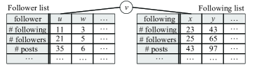
Figure 2: Graph properties maintained by vertex $v$.

Denote $\text{outdeg}(v)$ as the number of vertices that vertex $v$ follows, and by $\text{indeg}(v)$ is the number of vertices that follow $v$. To remove the sampling bias for observing high degree vertices’ graph properties, we use WCE to estimate vertex label density $\mbox{\boldmath$\tau$}=(\tau_{0},\ldots,\tau_{K^{\prime}})$ defined in Section 2, where $\tau_{k}$ ($0\leq k\leq K^{\prime}$) is the fraction of vertices with vertex label $l_{k}^{\prime}$. The property summary of each vertex $v$ can be viewed as content with $f^{\prime}(v)=\text{indeg}(v)+\text{outdeg}(v)+1$ copies maintained by the followers, following of $v$ and $v$ itself. For a collected vertex $v$, define its associated vertices $C^{\prime}(v)$ as the collection of its following, its followers, and itself. Note that $C^{\prime}(v)$ might contain duplicate elements since a vertex can be both the following and follower of $v$. We use WCE to estimate $\tau_{k}$ ($0\leq k\leq K^{\prime}$) as follows

$$\hat{\tau}_{k}^{\text{WCE}}=\frac{1}{S^{\prime}}\sum_{i=1}^{n}\sum_{v\in C^{\prime}(s_{i})}\frac{\mathbf{1}(L^{\prime}(v)=l_{k}^{\prime})}{\hat{\pi}_{s_{i}}f^{\prime}(v)},$$ (5)

where $S^{\prime}\!\!=\!\!\sum_{i=1}^{n}\sum_{v\in C^{\prime}(s_{i})}\frac{1}{\hat{\pi}_{s_{i}}f^{\prime}(v)}$. Note that $\hat{\tau}_{k}^{\text{WCE}}$ is an asymptotically unbiased estimator of $\tau_{k}$. To see that, we have the following equation for each $k=0,\ldots,K^{\prime}$ and $i=1,\ldots,n$

$$\begin{split}&\text{E}\left[\sum_{v\in C^{\prime}(s_{i})}\frac{\mathbf{1}(L^{\prime}(v)=l^{\prime}_{k})}{\hat{\pi}_{s_{i}}f^{\prime}(v)}\right]\\ &=\sum_{u\in V}\pi_{u}\sum_{v\in C^{\prime}(u)}\frac{\mathbf{1}(L^{\prime}(v)=l^{\prime}_{k})}{\hat{\pi}_{v}f^{\prime}(v)}\\ &=S_{\pi}\sum_{u\in V}\sum_{v\in C^{\prime}(u)}\frac{\mathbf{1}(L^{\prime}(v)=l^{\prime}_{k})}{f^{\prime}(v)}\\ &=S_{\pi}\sum_{u\in V}\mathbf{1}(L^{\prime}(v)=l^{\prime}_{k})=S_{\pi}|V|\tau_{k}.\end{split}$$

Then we have

$$\lim_{n\rightarrow\infty}\frac{1}{n}\sum_{i=1}^{n}\sum_{v\in C^{\prime}(s_{i})}\frac{\mathbf{1}(L^{\prime}(v)=l^{\prime}_{k})}{\hat{\pi}_{s_{i}}f^{\prime}(v)}\xrightarrow{a.s.}S_{\pi}|V|\tau_{k}.$$

Similarly, we have $\lim_{n\rightarrow\infty}\frac{S^{\prime}}{n}\xrightarrow{a.s.}S_{\pi}|V|$. Therefore $\hat{\tau}_{k}^{\text{WCE}}$ is an asymptotically unbiased estimator of $\tau_{k}$.

4 Data Evaluation

Our experiments are performed on a variety of real world networks, which are summarized in Table II. Xiami is a popular website devoted to music streaming and music recommendations. Similar to Twitter, Xiami builds a social network based on follower and following relationships. Each user has a numeric ID that is sequentially assigned. We crawled its entire network graph and have made the dataset publicly available. Flickr and YouTube are popular photo sharing and video sharing websites. In these websites, a user can subscribe to other user updates such as blogs and photos. These networks can be represented by a direct graph, with vertices representing users and a directed edge from $u$ to $v$ represents that user $u$ subscribes to user $v$. Further details of these datasets can be found in [27].

TABLE II: Overview of directed graph datasets used in our simulations.

Graph	Xiami	YouTube	Flickr
vertices	1,753,690	1,138,499	1,715,255
edges	16,019,106	2,990,443	15,555,041
directed-edges	16,574,010	4,945,382	22,613,981
vertices (LCC)	1,748,010	1,134,890	1,624,992
edges (LCC)	16,015,779	2,987,624	15,476,835
directed-edges (LCC)	16,568,449	4,942,035	22,477,015

“directed-edges” refers to the number of directed edges in a directed graph, “edges” refers to the number of edges in an undirected graph, and “LCC” refers to the largest connected component of a given graph.

Using real graph topologies which are publicly available, we generate benchmark datasets for our simulation experiments by manually generating content and distributing them over these graphs. In the following experiments we generate $10^{7}$ distinct content and distribute each content $\mathbf{c}$ using four different content distribution schemes (CDSs): CDS I, CDS II, CDS III, and CDS IV, which model information distribution mechanisms for undirected and directed graphs.

CDS I and II distribute content with a target content distribution by the number of copies. Define the truncated Pareto distribution as $\phi_{k}=\frac{\alpha}{\gamma k^{\alpha+1}}$, $k=1,\ldots,W$, where $\alpha>0$ and $\gamma=\sum_{k=1}^{W}\frac{\alpha}{k^{\alpha+1}}$ and $W$ is the maximum number of duplication. The number of copies for each content $\mathbf{c}$ is randomly selected from set $\{1,\ldots,W\}$ according to the truncated Pareto distribution with parameter $\alpha$ and $W$ for CDS I and II. Then copies of $\mathbf{c}$ are distributed as follows

$\bullet$ CDS I: We distribute each content copy to a randomly selected vertex in $G_{d}$ (one of the directed graph in Table II).

$\bullet$ CDS II: When content has $k$ copies, we first randomly select a vertex $v$ that can reach at least $k-1$ other vertices. In here, two vertices are reachable if there is at least one path between them in the undirected graph $G$, which is derived from $G_{d}$ by ignoring the direction of edges. Then we assign the special (or original) copy of this content to $v$, and assign $k-1$ duplicated copies to the top $k-1$ nearest vertices in $G$ which are reachable from $v$.

CDS III and CDS IV distribute each content $\mathbf{c}$ using the independent cascade model [28], that is

$\bullet$ CDS III: We distribute $\mathbf{c}$ over the associated undirected graph $G$. We first distribute the special copy of $\mathbf{c}$ to a randomly selected vertex $v$. Then we distribute copies of $\mathbf{c}$ to other vertices iteratively. When a new vertex first receives a copy of $\mathbf{c}$, it is given a single chance to distribute a copy of $\mathbf{c}$ to each of its neighbors currently without $\mathbf{c}$ with probability $p_{S}$.

$\bullet$ CDS IV: We distribute $\mathbf{c}$ similar to CDS III but on the direct graph $G_{d}$. The difference is that when a new vertex first receives a copy of $\mathbf{c}$, it is given a single chance to distribute a copy of $\mathbf{c}$ to each of its incoming neighbors (followers) currently without $\mathbf{c}$ with probability $p_{S}$.

Here we assume that each copy of content $\mathbf{c}$ records the number of copies possessed by $\mathbf{c}$ finally. In the following experiments we evaluate the performance of our methods for estimating $\omega$, content distribution by the number of copies. Let

$$NMSE(\hat{\omega}_{j})=\frac{\sqrt{\text{E}[(\hat{\omega}_{j}-\omega_{j})^{2}]}}{\omega_{j}}\,,j=1,2,\dots\,,$$

be a metric that measures the relative error of the estimate $\hat{\omega}_{j}$ with respect to its true value $\omega_{j}$. In our experiment, we average the estimates and calculate their NMSE over 1,000 runs. Let $B$ denote the sampling budget, which is the number of distinct sampled vertices per run. In the following experiments, we set default parameters as follows: sampling budget $B=0.01|V|$, uniform vertex sampling cost $c=1$, the number of random walkers $T=1000$ for FS. RW, MHRW and FS are evaluated on the LCC of graphs. UNI and RWJ are evaluated on the entire graphs. To simplify notation, graph sampling method A combined with content estimator B is denoted as method A_B.

Fig 3 shows the average of content distribution estimates of 1,000 runs for methods DCE, MLE, SCE and WCE. where the graph sampling method is UNI, content distribution scheme is CDS I, with $\alpha=1$, $W=\{20,50\}$. We observe that DCE is highly biased, while SCE and WCE are unbiased. MLE needs to sample most vertices to reduce biases especially for large $W$. Note that it SCE and WCE practically coincide with the correct values.

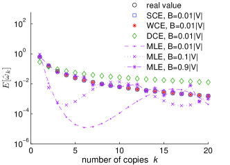
(a) $W=20$

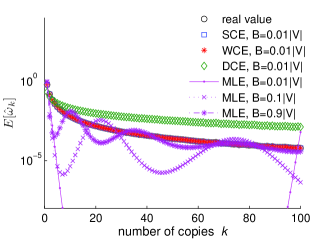
(b) $W=100$

Figure 3: (Xiami) Average of content distribution estimates for different estimators.

In the following experiments, we set $\alpha=1$, $W=10^{5}$ for CDS I and CDS II, $p_{S}=0.01$ for CDS III and CDS IV. We evaluate the performance of SCE and WCE combined with different graph sampling methods based on the datasets generated by four different CDS. Figs. 4 (a)–(d) show the complementary cumulative distribution function (CCDF) of the expectation of content distribution estimates provided by DCE, SCE and WCE, where the graph is Xiami and the graph sampling method is UNI. We find that DCE exhibits large errors, and SCE and WCE are quite accurate. Similar results are obtained when we use the other four graph sampling methods described in Section 2, but due to page limits, we omit them here. Figs. 4 (e)–(t) show the NMSE of SCE and WCE combined with different graph sampling methods for measuring content distribution. The results show that WCE is significantly more accurate than SCE over most points. In particular, WCE is almost an order of magnitude more accurate than SCE for the number of copies larger than 100, and nearly two orders of magnitude more accurate than SCE for the number of copies larger than 1,000. Fig. 5 show the compared results for different graph sampling methods where the graph used is the LCC of Xiami. The results show that UNI is quite accurate and MHRW exhibits large errors for content with a small number of copies. The compared results for WCE show that MHRW is much worse than the other graph sampling methods, while RW and FS have almost the same accuracy. The results for the graph YouTube are similar and are shown in [29].

(a) CDS I

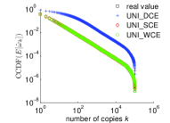
(b) CDS II

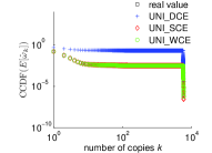
(c) CDS III

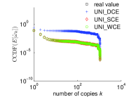
(d) CDS IV

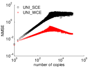
(e) UNI, CDS I

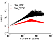
(f) RW, CDS I

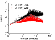
(g) MHRW, CDS I

(h) FS, CDS I

(i) UNI, CDS II

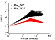
(j) RW, CDS II

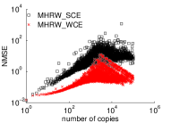
(k) MHRW, CDS II

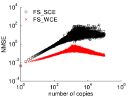
(l) FS, CDS II

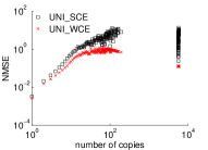
(m) UNI, CDS III

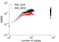
(n) RW, CDS III

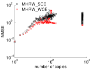
(o) MHRW, CDS III

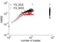
(p) FS, CDS III

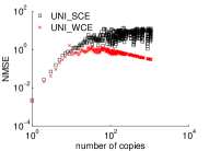
(q) UNI, CDS IV

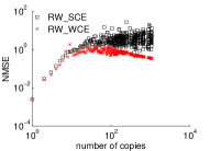
(r) RW, CDS IV

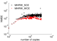
(s) MHRW, CDS IV

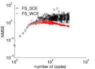
(t) FS, CDS IV

Figure 4: (Xiami) NMSE of content distribution estimates for different estimators and graph sampling methods.

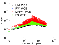
(a) CDS I

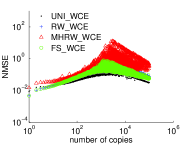
(b) CDS II

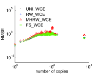
(c) CDS III

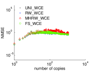
(d) CDS IV

Figure 5: (LCC of Xiami) Compared NMSE of content distribution estimates for WCE using different graph sampling methods.

Fig. 6 shows the distributions of users in Xiami using different labels, where the province numbers and corresponding names are shown in Table III. The fraction of users with more than $10^{4}$ followers, following, or recommendations is smaller than $2\times 10^{-6}$. The top three popular provinces are Guangdong, Beijing, and Shanghai. Similar results are also observed for the LCC of Xiami. Figs. 7 to 10 show the results of our new method to estimate these vertex label densities. The results show that WCE significantly outperforms the previous methods over almost all points. This is because WCE uses neighbors’ graph property summaries of sampled vertices. Especially for UNI_WCE, which is an order of magnitude more accurate than UNI for follower/following counts larger than 100. Fig. 11 show the compared results for different graph sampling methods where the graph used is the LCC of Xiami. The results show that MHRW is quite accurate. RW and FS almost have the same accuracy. For the follower and recommendation count distributions, UNI is more accurate for follower and recommendation counts with small values. Moreover Figs. 12 and 13 show the results for estimating out-degree distribution for YouTube and Flickr respectively. We observe that WCE is better than previous methods over almost all points.

TABLE III: (Xiami) Province numbers and corresponding names.

1. Beijing	2. Tianjin	3. Hebei
4. Shanxi	5. Inner Mongolia	6. Liaoning
7. Jilin	8. Heilongjiang	9. Shanghai
10. Jiangsu	11. Zhejiang	12. Anhui
13. Fujian	14. Jiangxi	15. Shandong
16. Henan	17. Hubei	18. Hunan
19. Guangdong	20. Guangxi	21. Hainan
22. Chongqing	23. Sichuan	24. Guizhou
25. Yunnan	26. Tibet	27. Shannxi
28. Gansu	29. Qinghai	30. Ningxia
31. Xinjiang	32. Taiwan	33. Hong Kong
34. Macao	35. Null	36. Overseas

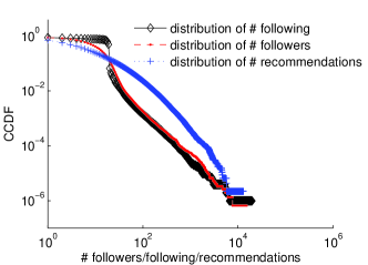
(a) # followers, # following, and # recommendations

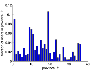
(b) Location

Figure 6: (Xiami) The distributions of users by different labels.

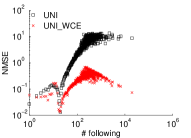
(a) UNI_WCE vs. UNI

(b) RW_WCE vs. RW

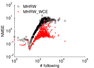
(c) MHRW_WCE vs. MHRW

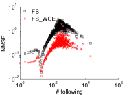
(d) FS_WCE vs. FS

Figure 7: NMSE of following count distribution estimates.

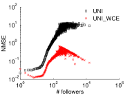
(a) UNI_WCE vs. UNI

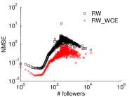
(b) RW_WCE vs. RW

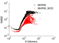
(c) MHRW_WCE vs. MHRW

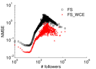
(d) FS_WCE vs. FS

Figure 8: (Xiami) NMSE of follower count distribution estimates.

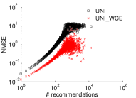
(a) UNI_WCE vs. UNI

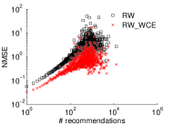
(b) RW_WCE vs. RW

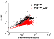
(c) MHRW_WCE vs. MHRW

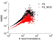
(d) FS_WCE vs. FS

Figure 9: (Xiami) NMSE of recommendation count distribution estimates.

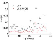
(a) UNI_WCE vs. UNI

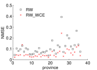
(b) RW_WCE vs. RW

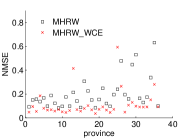
(c) MHRW_WCE vs. MHRW

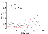
(d) FS_WCE vs. FS

Figure 10: (Xiami) NMSE of location distribution estimates.

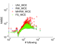
(a) # following

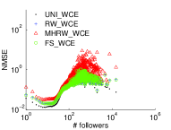
(b) # follower

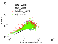
(c) # recommendation

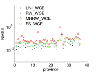
(d) Location

Figure 11: (LCC of Xiami) Compared NMSE of graph label density estimates for WCE using different graph sampling methods.

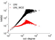
(a) UNI_WCE vs. UNI

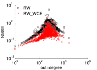
(b) RW_WCE vs. RW

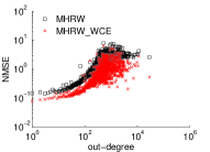
(c) MHRW_WCE vs. MHRW

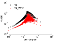
(d) FS_WCE vs. FS

Figure 12: (YouTube) NMSE of out-degree distribution estimates.

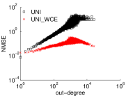
(a) UNI_WCE vs. UNI

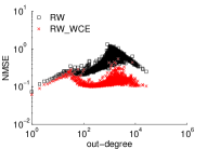
(b) RW_WCE vs. RW

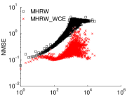
(c) MHRW_WCE vs. MHRW

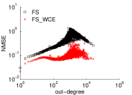
(d) FS_WCE vs. FS

Figure 13: (Flickr) NMSE of out-degree distribution estimates.

5 Applications

We now apply our methodology to a real OSN to characterize various content, i.e., average number of retweets or replies per tweet, types of tweet messages, as well as the associated top rank statistics. We perform experiments on Sina microblog network. By crawling webpages of 148,313 random accounts selected by UNI, we obtain 19.7 million tweets and retweets. Note that in the following analysis, tweets refer to the original tweets. Each tweet or retweet records its original tweet’s information such as the number of retweets and replies. Fig. 14 shows the results of estimating the distribution of tweets from retweets and replies using DCE, SCE and WCE, where the special content is defined as the original tweet for SCE. The estimates for the average number of retweets and replies per tweet are shown as Table IV. We observe that the estimates of SCE and WCE are close to each other, but the estimates obtained by DCE significantly deviate from SCE and WCE. This is consistent with previous simulation results which show that DCE introduces large biases. Furthermore, Fig. 14 shows that the maximum number of retweets or replies given by SCE is the smallest since it only uses information of sampled original tweets, and the original tweets of popular tweets are not always sampled.

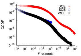
(a) # retweets

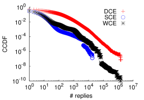
(b) # replies

Figure 14: Distributions of tweets by the number of rewteets and replies.

TABLE IV: Estimates of the average number of rewteets and replies per tweet by different methods

	Avg. # retweets	Avg. # replies
DCE	423	89.8
SCE	2.01	3.93
WCE	1.60	4.60

Let us explore the “type” of tweets. We classify tweets into three types:text tweet, image tweet, and video tweet. Table V shows their statistics measured by WCE. We find that 60.1% are text tweets, 37.6% are image tweets, and 2.3% are video tweets. On average, image and video tweets have more retweets and replies than text tweets. Table VI shows the statistics of video tweets by their associated external video source websites. We find that the top five popular video websites are youku.com (42.7%), tudou.com (26.3%), sina.com (10.0%), yinyuetai.com (6.2%) and 56.com (4.4%).

TABLE V: (Sina microblog) Statistics of tweets by different categories

	Fraction of	Avg. # retweets	Avg. # replies
	tweets	per tweet	per tweet
Text	60.1%	0.31	2.30
Image	37.6%	3.33	7.91
Video	2.3%	7.05	10.91

TABLE VI: (Sina microblog) Statistics of video tweets

Source	Fraction of	Avg.	Avg.
	video	# retweets	# replies
	tweets	per tweet	per tweet
youku.com	42.7%	5.57	9.68
tudou.com	26.3%	9.87	13.73
sina.com	10.0%	9.09	11.32
yinyuetai.com	6.2%	5.06	9.36
56.com	4.4%	11.29	26.64
ku6.com	2.9%	11.29	13.02
sohu.com	1.7%	4.56	1.29
kandian.com	1.6%	0.13	0.16
baomihua.com	1.6%	0.31	0.08
ifeng.com	0.9%	5.77	4.36

6 Related Work

Previous graph sampling work focuses on designing accurate and efficient sampling methods for measuring graph characteristics, such as vertex degree distribution [12, 23, 4, 5, 15] and the topology of vertices’ groups [30]. We summarize previous graph sampling work as follows: Most previous OSN graph crawling and sampling work focuses on undirected graph since each vertex in most OSNs maintains both its incoming and outgoing neighbors, so it is easy to convert these directed OSNs to their associated undirected graphs by ignoring the directions of edges. Breadth-First-Search (BFS), though it is easy to implement but it introduces a large bias towards high degree vertices, and it is difficult to remove these biases in general [10, 11, 31]. Random walk (RW) is biased to sample high degree vertices, however its bias is known and can be corrected [17, 18]. Compared with uniform vertex sampling (UNI), a RW has smaller estimation errors for high degree vertices, and these vertices are quite common for many OSNs like Facebook, Myspace and Flickr [5]. Furthermore, it is costly to apply UNI in these networks. The Metropolis-Hasting RW (MHRW) [19, 12, 4] modifies the RW procedure, and it aims to sample each vertex with the same probability. The accuracy of RW and MHRW is compared in [23, 4]. RW is shown to be consistently more accurate than MHRW. The mixing time of a RW determines the efficiency of the sampling, and it is found to be much larger than commonly believed for many OSNs [32]. There are a lot of work on how to decrease the mixing time [33, 5, 34, 35, 36]. To sample a directed graph with latent incoming links (e.g. the Web graph and Flickr [13]),  [37] and [38] apply a MHRW over an undirected graph which is built on-the-fly by adding observed links from the directed graph. However, these algorithms are biased since the generated undirected graph may not contain all vertices in the original directed graph. To address this issue, Ribeiro et al. [15] use a RW with jumps under the assumption that vertices can be uniformly sampled at random from directed graphs. To the best of our knowledge, our work is the first to study the problem of measuring characteristics of content distributed over large graphs based on graph sampling techniques.

7 Conclusions

In this paper, we study the problem of estimating characteristics of content distributed over large graphs. The analysis and experiment results show that existing graph sampling methods are biased to sample content with a large number of copies, and there can be huge bias in statistics computed by directly using collected content. To remove this bias, the MLE method is applied. However, we show that MLE needs to sample most vertices in the graph to obtain accurate statistics. To address this challenge, we propose two efficient methods SCE and WCE using available information in sampled content. We show that they are asymptotically unbiased. We perform extensive measurement and experiments, and show that WCE is more accurate than SCE. Furthermore, we use WCE to estimate graph characteristics when vertices maintain their neighbors’ graph properties. We carry out experiments to show that WCE is more accurate than previous sampling methods.

Pinghui Wang received the B.S. degree in information engineering and Ph.D degree in automatic control from Xi’an Jiaotong University, Xi’an, China, in 2006, 2012 respectively. From April 2012 to October 2012, he was a postdoctoral researcher with the Department of Computer Science and Engineering at The Chinese University of Hong Kong. He is currently a postdoctoral researcher with School of Computer Science at McGill University, QC, Canada. His research interests include Internet traffic measurement and modeling, traffic classification, abnormal detection, and online social network measurement.

Junzhou Zhao received the B.S. degree in automatic control from Xi’an Jiaotong University, Xi’an, China, in 2008. He is currently a Ph.D. candidate with the Systems Engineering Institute and MOE Key Lab for Intelligent Networks and Network Security, Xi’an Jiaotong University under the supervision of Prof. Xiaohong Guan. His research interests include online social network measurement and modeling.

John C.S. Lui received the PhD degree in computer science from UCLA. He is currently a professor in the Department of Computer Science and Engineering at The Chinese University of Hong Kong. His current research interests include communication networks, networksystem security (e.g., cloud security, mobile security, etc.), network economics, network sciences (e.g., online social networks, information spreading, etc.), cloud computing, large-scale distributed systems and performance evaluation theory. He serves in the editorial board of IEEEACM Transactions on Networking, IEEE Transactions on Computers, IEEE Transactions on Parallel and Distributed Systems, Journal of Performance Evaluation and International Journal of Network Security. He was the chairman of the CSE Department from 2005-2011. He received various departmental teaching awards and the CUHK Vice-Chancellor s Exemplary Teaching Award. He is also a corecipient of the IFIP WG 7.3 Performance 2005 and IEEEIFIP NOMS 2006 Best Student Paper Awards. He is an elected member of the IFIP WG 7.3, fellow of the ACM, fellow of the IEEE, and croucher senior research fellow. His personal interests include films and general reading.

Don Towsley holds a B.A. in Physics (1971) and a Ph.D. in Computer Science (1975) from University of Texas. From 1976 to 1985 he was a member of the faculty of the Department of Electrical and Computer Engineering at the University of Massachusetts, Amherst. He is currently a Distinguished Professor at the University of Massachusetts in the Department of Computer Science. He has held visiting positions at IBM T.J. Watson Research Center, Yorktown Heights, NY; Laboratoire MASI, Paris, France; INRIA, Sophia-Antipolis, France; AT&T Labs-Research, Florham Park, NJ; and Microsoft Research Lab, Cambridge, UK. His research interests include networks and performance evaluation. He currently serves as Editor-in-Chief of IEEE/ACM Transactions on Networking and on the editorial boards of Journal of the ACM, and IEEE Journal on Selected Areas in Communications, and has previously served on numerous other editorial boards. He was Program Co-chair of the joint ACM SIGMETRICS and PERFORMANCE 92 conference and the Performance 2002 conference. He is a member of ACM and ORSA, and Chair of IFIP Working Group 7.3. He has received the 2007 IEEE Koji Kobayashi Award, the 2007 ACM SIGMETRICS Achievement Award, the 1998 IEEE Communications Society William Bennett Best Paper Award, and numerous best conference/workshop paper awards. Last, he has been elected Fellow of both the ACM and IEEE.

Xiaohong Guan received the B.S. and M.S. degrees in automatic control from Tsinghua University, Beijing, China, in 1982 and 1985, respectively, and the Ph.D. degree in electrical engineering from the University of Connecticut, Storrs, US, in 1993. From 1993 to 1995, he was a consulting engineer at PG&E. From 1985 to 1988, he was with the Systems Engineering Institute, Xi’an Jiaotong University, Xi’an, China. From January 1999 to February 2000, he was with the Division of Engineering and Applied Science, Harvard University, Cambridge, MA. Since 1995, he has been with the Systems Engineering Institute, Xi’an Jiaotong University, and was appointed Cheung Kong Professor of Systems Engineering in 1999, and dean of the School of Electronic and Information Engineering in 2008. Since 2001 he has been the director of the Center for Intelligent and Networked Systems, Tsinghua University, and served as head of the Department of Automation, 2003-2008. He is an Editor of IEEE Transactions on Power Systems and an Associate Editor of Automata. His research interests include allocation and scheduling of complex networked resources, network security, and sensor networks. He has been elected Fellow of IEEE.

References

- [1] B. Suh, L. Hong, P. Pirolli, and E. H. Chi, “Want to be retweeted? large scale analytics on factors impacting retweet in twitter network,” in Proceedings of IEEE International Conference on Social Computing 2010, Augest 2010, pp. 177–184.
- [2] Z. Li, H. Shen, H. Wang, G. Liu, and J. Li, “Socialtube: P2p-assisted video sharing in online social networks,” in Proceedings of IEEE INFOCOM Mini Conference 2012, April 2012, pp. 2886–2890.
- [3] F. Malandrino, M. Kurant, A. Markopoulou, C. Westphal, and U. C. Kozat, “Proactive seeding for information cascades in cellular networks,” in Proceedings of IEEE INFOCOM 2012, April 2012, pp. 2886–2890.
- [4] M. Gjoka, M. Kurant, C. T. Butts, and A. Markopoulou, “Walking in facebook: A case study of unbiased sampling of OSNs,” in Proceedings of IEEE INFOCOM 2010, April 2010, pp. 2498–2506.
- [5] B. Ribeiro and D. Towsley, “Estimating and sampling graphs with multidimensional random walks,” in Proceedings of ACM SIGCOMM Internet Measurement Conference 2010, November 2010, pp. 390–403.
- [6] “Renren,” http://www.renren.com, 2012.
- [7] “Sina microblog,” http://weibo.com, 2012.
- [8] “Xiami,” http://www.xiami.com, 2012.
- [9] M. Yang, H. Chen, B. Y. Zhao, Y. Dai, and Z. Zhang, “Deployment of a large-scale peer-to-peer social network,” in In Proc. of WORLDS, 2004.
- [10] D. Achlioptas, D. Kempe, A. Clauset, and C. Moore, “On the bias of traceroute sampling or, power-law degree distributions in regular graphs,” in Symposium on Theory of Computing 2005, May 2005, pp. 694–703.
- [11] M. Kurant, A. Markopoulou, and P. Thiran, “On the bias of bfs (breadth first search) and of other graph sampling techniques,” in Proceedings of International Teletraffic Congress 2010, September 2010.
- [12] D. Stutzbach, R. Rejaie, N. Duffield, S. Sen, and W. Willinger, “On unbiased sampling for unstructured peer-to-peer networks,” IEEE/ACM Transactions on Networking, vol. 17, no. 2, pp. 377–390, April 2009.
- [13] “Flickr,” http://www.flickr.com, July 2010.
- [14] B. Ribeiro, W. Gauvin, B. Liu, and D. Towsley, “On myspace account spans and double pareto-like distribution of friends,” in Proceedings of IEEE Infocom NetSciCom Workshop, April 2010, pp. 1–6.
- [15] B. Ribeiro, P. Wang, F. Murai, and D. Towsley, “Sampling directed graphs with random walks,” in Proceedings of IEEE INFOCOM 2012, April 2012, pp. 1692–1700.
- [16] L. Lovász, “Random walks on graphs: a survey,” Combinatorics, vol. 2, pp. 1–46, 1993.
- [17] D. D. Heckathorn, “Respondent-driven sampling II: deriving valid population estimates from chain-referral samples of hidden populations,” Social Problems, vol. 49, no. 1, pp. 11–34, 2002.
- [18] M. J. Salganik and D. D. Heckathorn, “Sampling and estimation in hidden populations using respondent-driven sampling,” Sociological Methodology, vol. 34, pp. 193–239, 2004.
- [19] M. Zhong and K. Shen, “Random walk based node sampling in self-organizing networks,” ACM SIGOPS Operating Systems Review, vol. 40, no. 3, pp. 49–55, July 2006.
- [20] S. Chib and E. Greenberg, “Understanding the metropolis-hastings algorithm,” The American Statistician, vol. 49, no. 4, pp. 327–335, November 1995.
- [21] W. K. Hastings, “Monte carlo sampling methods using markov chains and their applications,” Biometrika, vol. 57, no. 1, pp. 97–109, April 1970.
- [22] N. Metropolis, A. W. Rosenbluth, M. N. Rosenbluth, A. H. Teller, and E. Teller, “Equations of state calculations by fast computing machines,” IEEE Journal on Selected Areas in Communications, vol. 21, no. 6, pp. 1087–1092, June 2011.
- [23] A. H. Rasti, M. Torkjazi, R. Rejaie, N. Duffield, W. Willinger, and D. Stutzbach, “Respondent-driven sampling for characterizing unstructured overlays,” in Proceedings of IEEE INFOCOM Mini-conference 2009, April 2009.
- [24] L. Katzir, E. Liberty, and O. Somekh, “Estimating sizes of social networks via biased sampling,” in Proceedings of WWW 2011, March 2011, pp. 597–606.
- [25] N. Duffield, C. Lund, and M. Thorup, “Estimating flow distributions from sampled flow statistics,” in Proceedings of ACM SIGCOMM 2003, August 2003, pp. 325–336.
- [26] F. Murai, B. Ribeiro, D. Towsley, and P. Wang, “On set size distribution estimation and the characterization of large networks via sampling,” in arXiv:1209.0736.
- [27] A. Mislove, M. Marcon, K. P. Gummadi, P. Druschel, and B. Bhattacharjee, “Measurement and analysis of online social networks,” in Proceedings of ACM SIGCOMM Internet Measurement Conference 2007, October 2007, pp. 29–42.
- [28] J. Goldenberg, B. Libai, and E. Muller, “Talk of the network: A complex systems look at the underlying process of word-of-mouth,” Marketing Letters, vol. 12, no. 3, pp. 211–223, 2001.
- [29] P. Wang, J. Zhao, J. C. Lui, D. Towsley, and X. Guan, “Sampling content distributed over graphs, available at www.cse.cuhk.edu.hk/%7ecslui/samplingcontentreport.pdf,” The Chinese University of Hong Kong, Tech. Rep., 2012.
- [30] M. Kurant, M. Gjoka, Y. Wang, Z. W. Almquist, C. T. Butts, and A. Markopoulou, “Coarse-grained topology estimation via graph sampling,” in arXiv:1105.5488, 2011.
- [31] M. Kurant, A. Markopoulou, and P. Thiran, “Towards unbiased bfs sampling,” IEEE Journal on Selected Areas in Communications, vol. 29, no. 9, pp. 1799–1809, September 2011.
- [32] A. Mohaisen, A. Yun, and Y. Kim, “Measuring the mixing time of social graphs,” in Proceedings of ACM SIGCOMM Internet Measurement Conference 2010, November 2010, pp. 390–403.
- [33] S. Boyd, P. Diaconis, and L. Xiao, “Fastest mixing markov chain on a graph,” SIAM Review, vol. 46, no. 4, pp. 667–689, December 2004.
- [34] K. Avrachenkov, B. Ribeiro, and D. Towsley, “Improving random walk estimation accuracy with uniform restarts,” in The 7th Workshop on Algorithms and Models for the Web Graph, December 2010, pp. 98–109.
- [35] M. Gjoka, C. T. Butts, M. Kurant, and A. Markopoulou, “Multigraph sampling of online social networks,” IEEE Journal on Selected Areas in Communications, vol. 29, no. 9, pp. 1893–1905, September 2011.
- [36] M. Kurant, M. Gjoka, C. T. Butts, and A. Markopoulou, “Walking on a graph with a magnifying glass: Stratified sampling via weighted random walks,” in Proceedings of ACM SIGMETRICS 2011, June 2011, pp. 281–292.
- [37] Z. Bar-Yossef and M. Gurevich, “Random sampling from a search engine’s index,” Journal of the ACM, vol. 55, no. 5, pp. 1–74, 2008.
- [38] M. R. Henzinger, A. Heydon, M. Mitzenmacher, and M. Najork, “On near-uniform url sampling,” in Proceedings of the WWW, May 2000, pp. 295–308.