Solutions to position-dependent mass quantum mechanics for a new class of hyperbolic potentials

Abstract

We analytically solve the position-dependent mass (PDM) 1D Schrödinger equation for a new class of hyperbolic potentials $V_{q}^{p}(x)=-V_{0}\frac{\sinh^{p}x}{\cosh^{q}x},\,p=-2,0,\dots q$ [see C. A. Downing, J. Math. Phys. 54 072101 (2013)] among which several hyperbolic single- and double-wells. For a solitonic mass distribution, $m(x)=m_{0}\,\operatorname{sech}^{2}(x)$, we obtain exact analytic solutions to the resulting differential equations. For several members of the class, the quantum mechanical problems map into confluent Heun differential equations. The PDM Poschl-Teller potential is considered and exactly solved as a particular case.

I Introduction

The dynamics of quantum systems has been extensively studied in connection with countless problems of physics, from low to high energies, since the beginnings of the last century. Non-relativistic quantum particles are accurately described by a Schrödinger equation whose difficulties exclusively depend on the potential function associated with the external background. Mathematically, the problem consists in dealing with the resulting differential equation which, for stationary systems, winds up in an eigenvalue problem in a Hilbert space cohen . Exact solutions of solvable potentials have been generally found in terms of polynomials, exponential, trigonometric, hyperbolic, hypergeometric and even elliptic functions morse ; eckart ; rosenmorse ; manningrosen ; poschlteller ; manning ; ma47 ; bargmann ; scarf ; ff61 ; cimento62 ; cimento64 ; CPM66 ; natanzon79 ; nieto78 ; prl83 ; gino84 .

Although the number of exactly solvable potentials has been slowly growing up along the last nighty years, as soon as we switch the traditionally constant mass into a position-dependent distribution the mathematical challenge becomes dramatically different. Notwithstanding, a few phenomenological potentials with appropriate mass distributions have been worked out in recent years and their solutions have also been found proportional to special functions ardasever2011 ; iran ; severtezcan ; midyaroy2009 ; bagchi .

Historically, a crucial motivation for the PDM approximation came from many-body problems in solid state and condensed matter physics wannier ; slater ; luttingerkohn ; BDD ; bastard81 ; vonroos ; einehem88 ; levy95 . One example is the effective-mass model related to the envelope-function approximation used to study the dynamics of electrons in semiconductor heterostructures BDD ; zhukro83 ; weisvin91 .

In fact, particles with spatially dependent distributions of mass have been investigated in several relevant subjects of low-energy physics related to the understanding of the electronic properties of semiconductor heterostructures, crystal-growth techniques gorawill ; bastardetal ; bastard88 , quantum wells and quantum dots dots , Helium clusters helium , graded crystals prl93 , quantum liquids qliq , etc., and has recently been shown to be appropriate for the description of growth-intended geometrical nanowire structures suffering size variations, impurities, dislocations, and geometry imperfections willatzenlassen2007 .

In connection with the mathematical aspects of the PDM issue, here we focus on the class of solutions of the effective PDM Schrödinger equation for a family of potentials

$$V_{p,q}(x)=-V_{0}\frac{\sinh^{p}(x/d)}{\cosh^{q}(x/d)},\,p=-2,0,\dots q$$ (1)

reported a few months ago in the usual constant mass framework downing (see Sec. II.2 for details). There, it is claimed that for this potentials class the equation cannot be necessarily transformed into any hypergeometric special case abramowitz as traditionally covet, and it is shown that for $q=4,6$ the Schrödinger equation is equivalent to a confluent Heun equation heun , more difficult to handle maier ; maier192 ; conflu ; ronveaux ; hille ; slavyanov ; hounkonnou ; fiziev and not so well-known as the above mentioned. Actually, the author manages to compute the low lying spectrum for the case $(p,q)=(4,6)$.

In the present work we analyze this new family of potentials with a noteworthy modification, namely a nonuniform mass for the quantum particle, and we further explore several members of this class. This phenomenological upgrade of course induces highly nontrivial consequences in the associated differential equations and yields new physical models. Our goal is to analytically treat these resulting equations and find their solutions. We do it in several representative $(p,q)$ cases and find again confluent Heun equations (with new due entries) even where there were just hypergeometric ones for a constant mass. After a number of simple transformations we were able to obtain exact expression for their eigenstates.

In the next section, II.1, we digress about the question of which suitable differential operator one should consider to conveniently modify the Schrödinger equation for PDM. In Sec. II.2 we obtain an effective potential in a convenient space and in Sec. III we consider the $V_{(p,q)}(x)$ family of potentials and discuss one by one several $(p,q)$ representatives among which the hyperbolic PDM Poschl-Teller wells and the hyperbolic PDM double-well. Explicit wave-functions and eigenvalues are presented along with some selected graphics. In all the cases we take the constant mass limit and compare it with the results of Ref. downing . The final remarks are drawn in Sec.IV.

II The PDM Schrödinger equation

In this section we discuss the operational aspect of the effective hamiltonian of the quantum system when the mass of the particle is assumed to depend on the spatial coordinate.

II.1 Digression on the momentum operator

Since we want to consider a position-dependent mass $m(x)$ in the Schrödinger equation, an ordering problem arises from scratch with the momentum operator. Clearly, the $x$-representation of the momentum, $\hat{P}=-i\hbar\;d/dx$, demands considering derivatives not just on the wave-function but also on the mass. The consequences of such inherent ordering dilemma are in fact serious since a bunch of possibilities spreads out bastard81 ; vonroos ; einehem88 ; levy95 ; BDD ; zhukro83 ; gorawill ; shewell ; morrowbron84 ; vonroofmavro ; morrow ; galgeo ; likhun ; thomsenetc ; young ; einevol1 ; einevol2 ; tdlee ; DA

Instead of the ordinary kinetic-energy operator $\hat{T}_{0}=\frac{1}{2}m^{-1}\,\hat{P}^{2}$, a fully comprehensive operator allowing all such ordering possibilities reads

$$\hat{T}=\,\frac{1}{4}\,\hat{T}_{0}\,+\frac{1}{8}\left\{\,\,\hat{P}^{2}\,m^{-1}(x)+\,m^{\alpha}(x)\,\hat{P}\ m^{\beta}(x)\,\hat{P}\ m^{\gamma}(x)\,\,+\,m^{\gamma}(x)\,\hat{P}\ m^{\beta}(x)\,\hat{P}\ m^{\alpha}(x)\,\right\},$$ (2)

with $\alpha+\beta+\gamma=-1$ vonroos . Taking into account the commutation rules of Quantum Mechanics, $[\hat{X},\hat{P}]=i\hbar$, we get

$$\hat{T}\,=\,\frac{1}{2\,m}\,\hat{P}^{2}\,+\,\frac{i\hbar}{2}\frac{1}{m^{2}}\frac{dm}{dx}\,\,\hat{P}\,\,+\,U_{\rm K}\left(x\right),$$ (3)

where

$$U_{\rm K}\left(x\right)=\frac{-\hbar^{2}}{4m^{3}(x)}\left[\left(\alpha+\gamma-1\right)\frac{m(x)}{2}\left(\frac{d^{2}m}{dx^{2}}\right)+\left(1-\alpha\gamma-\alpha-\gamma\right)\left(\frac{dm}{dx}\right)^{2}\right]$$ (4)

is an effective potential of kinematic origin. Potential $U_{\rm K}$ is thus a source of an uncomfortable ambiguity in the hamiltonian of the physical problem since its spatial shape depends on the values of $\alpha,\beta,\gamma$.

Nevertheless, if we also constrain

$$\alpha\,+\,\gamma\,=\,1\,=\alpha\,\gamma\,+\,\alpha\,+\,\gamma$$ (5)

the kinetic operator $\hat{T}$ becomes unique. As an extra bonus one finds that the first-try symmetrized-Weyl order tdlee (viz. $\alpha\,=\,\gamma=\,0$) gets excluded in favor of the resulting, and most consensual, Ben-Daniel–Duke ordering BDD which is the one solution to the non-ambiguity condition Eq. (5) (viz. $\alpha=0$ and $\gamma=1$, or $\alpha=1$ and $\gamma=0$).

In any case, although free of the uncertainties of the kinematic potential (4), the new effective Schrödinger equation now includes a first order derivative term. For an arbitrary external potential $V(x)$ the PDM-Schrödinger equation thus reads

$$\left\{\frac{d^{2}}{dx^{2}}-\left(\frac{1}{m(x)}\frac{dm(x)}{dx}\right)\frac{d}{dx}+\frac{2}{\hbar^{2}}\,m(x)\,\big{[}E-V(x)\big{]}\right\}\psi(x)=0.$$ (6)

Noticeably, not only the last term has been strongly modified from the ordinary Schrödinger equation but the differential operator turned out to be dramatically changed. This will have of course deep consequences on the physical wave solution of the system.

II.2 The potentials

The potential functions we are dealing with are

$$V_{p,q}(x)=-V_{0}\frac{\sinh^{p}(x/d)}{\cosh^{q}(x/d)},\,p=-2,0,\dots q$$ (7)

where the depth $V_{0}$ and width $d$, and the family parameters $p$ and $q$, determine a plethora of possible shapes.

Here we adopt the following smooth effective mass distribution

$$m(x)=m_{0}\,\operatorname{sech}^{2}(x/d)$$ (8)

which mimics a solitonic mass density (see e.g. iran and bagchi ) familiar in effective models of condensed matter and low energy nuclear physics. The scale parameter $d$ widens the shape of the effective mass as it gets larger. Inversely, the mass and energy scales decrease as $d$ grow up, see Eq. (9). Now, the resulting Schrödinger equation reads

$$\psi^{\prime\prime}(x)+2\tanh(x)\psi^{\prime}(x)+\frac{2m_{0}d^{2}}{\hbar^{2}}(E-V_{p,q}(x))\,\operatorname{sech}^{2}(x)\psi(x)=0,$$ (9)

where we shifted $x/d\rightarrow x$. Trying the ansatz solution

$$\psi(x)=\cosh^{\nu}\!(x)\,\varphi(x),$$ (10)

Eq. (9) becomes

$$\varphi^{\prime\prime}(x)+2(\nu+1)\tanh(x)\varphi^{\prime}(x)+\left[\nu(\nu+2)\tanh^{2}\!x+\left(\nu+\frac{2m_{0}}{a^{2}\hbar^{2}}(E-V_{p,q}(x))\right)\,\operatorname{sech}^{2}(x)\right]\varphi(x)=0.$$ (11)

Now, we map the domain $(-\infty,\infty)\rightarrow(-\frac{\pi}{2},\frac{\pi}{2})$ by means of a change of variable $\textsf{sech}\,x=\cos\,z,$ getting

$$\varphi^{\prime\prime}(z)+(2\nu+1)\tan(z)\varphi^{\prime}(z)+\left[\nu+\nu(\nu+2)\tan^{2}(z)+\frac{2m_{0}d^{2}}{\hbar^{2}}\left(E-\tilde{V}_{p,q}(z)\right)\right]\varphi(z)=0.$$ (12)

Choosing $\nu=-1/2$ we can remove the first derivative and obtain

$$\left[-\frac{d^{2}}{dz^{2}}+\mathcal{V}_{p,q}(z)\right]\varphi(z)=\mathcal{E}\varphi(z)$$ (13)

where

$$\mathcal{V}_{p,q}(z)=\frac{1}{2}+\frac{3}{4}\tan^{2}\!z-\mathcal{V}_{0}\ {\tan^{p}\!z}\,{\cos^{q}\!z},$$ (14)

$\mathcal{E}=\frac{2m_{0}d^{2}}{\hbar^{2}}E$ and $\mathcal{V}_{0}=\frac{2m_{0}d^{2}}{\hbar^{2}}V_{0}$.

In this way, we transformed the differential equation (6) into a true ordinary Schrödinger equation, viz. Eq.(13), which governs the dynamics of a particle of constant mass $m_{0}$ moving in an effective potential free of any kinematical contribution. Now the dynamics is restricted to within $z=(-\frac{\pi}{2},\frac{\pi}{2})$ and $\varphi(z=\pm\frac{\pi}{2})=0$. Eventually, we can easily transform everything back to the original variable and wave-function to obtain the real space solution.

III Analysis of solutions: Heun functions

In this section we inspect one by one different members of this family of potentials allowing a position-dependent mass in the Schrödinger-like differential equation (6). As we will see, this class of problems has complicated solutions most of which are Heun functions of the confluent type. A confluent Heun differential equation arises from a general Heun equation under a procedure which consists in making diverge three of its six parameters while holding them proportional in a precise way. In its confluent form two or more regular singularities merge to give rise to an irregular singularity conflu . Notice that, as demonstrated in maier , a local Heun solution with four regular singular points can be reduced to a Gauss hypergeometric function with only three regular singular points in some cases. This will be explicitly shown in the first of the following family cases. The other constituents of the class have irreducible confluent Heun solutions as we will see next.

III.1 The case $(p,q)=(0,0)$

For $p=0$ and $q=0$ the potential $V_{(0,0)}(x)=-V_{0}$, which amounts to a $V(x)=0$ case without loss of generality. Thus, in a sense it belongs to all the family members. Although null, this is anyway a nontrivial situation as a result of the position-dependent mass. We have already studied this issue in cunha-christiansen2013 so we shall review it quickly. It will be helpful to show the relevant steps of our derivation and to exhibit the analytical procedure and its connection with the Heun equation as well.

We start directly with Eq. (13). Upon a second transformation of variables, $y=\cos z$, and with an ansatz solution $\varphi(y)=y^{-1/2}h_{1}(y)$, we obtain

$$h_{1}^{\prime\prime}(y)+\left(\frac{-1}{y}+\frac{{}^{1}\!/{}_{\!2}}{y-1}+\frac{{}^{1}\!/{}_{\!2}}{y+1}\right)h_{1}^{\prime}(y)+\frac{-k^{2}y}{y(y-1)(y+1)}h_{1}(y)=0\,\,$$ (15)

where $0<y<1$ and $k^{2}=2m_{0}d^{2}E/\hbar^{2}$. This equation belongs to the second order fuchsian class hille and can be recognized as a special case of the Heun equation ronveaux

$$H^{\prime\prime}(y)+\left(\frac{\gamma}{y}+\frac{\delta}{y-1}+\frac{\varepsilon}{y-d}\right)H^{\prime}(y)+\frac{\alpha\beta y-q}{y(y-1)(y-d)}H(y)=0\,\,$$ (16)

where the fuchsian relation $\alpha+\beta+1=\gamma+\delta+\varepsilon$ holds. We look for solutions around the singularity $y=1$, which corresponds to $x=0$ in the original space. For this the characteristic exponents are $0$ and $1-\delta$ and thus the two relevant linearly independent local Heun solutions to Eq.16 are

$$H^{(1)}=H(1-d,-q+\alpha\beta,\alpha,\beta,\delta,\gamma;1-y)$$

$$H^{(2)}=(1-y)^{1-\delta}\!H[1-d,-q+(\delta-1)\gamma d+(\alpha-\delta+1)(\beta-\delta+1),\beta-\delta+1,\alpha-\delta+1,2-\delta,\gamma;1-y].$$ (17)

III.1.1 Even solutions

Looking at Eq.(15) and Eq.(16) we identify $d=-1$, $q=0$, $\alpha=-{}^{1}\!/{}_{\!2}+{}^{1}\!/{}_{\!2}\sqrt{1+4k^{2}}$, $\beta=-{}^{1}\!/{}_{\!2}-{}^{1}\!/{}_{\!2}\sqrt{1+4k^{2}}$, $\gamma=-1$, $\delta={}^{1}\!/{}_{\!2}$ and $\varepsilon={}^{1}\!/{}_{\!2}$ which result in

$$h_{1}^{(1)}(y)=H\left(2,-k^{2},\frac{-1+\sqrt{1+4k^{2}}}{2},\frac{-1-\sqrt{1+4k^{2}}}{2},{}^{1}\!/{}_{\!2},-1;1-y\right)\leavevmode\nobreak\ \leavevmode\nobreak\ \leavevmode\nobreak\ \leavevmode\nobreak\$$ (18)

$$h_{1}^{(2)}(y)=(1\!-\!y)^{1/2}\!H\!\left(\!2,-\frac{3+4k^{2}}{4},-\frac{\sqrt{1+4k^{2}}}{2},\frac{\sqrt{1+4k^{2}}}{2},{}^{3}\!/{}_{\!2},\!-1;1\!-\!y\right)\leavevmode\nobreak\ \leavevmode\nobreak\$$ (19)

corresponding to

$$\psi^{(1,2)}(x)=h_{1}^{(1,2)}(\operatorname{sech}x)$$ (20)

in the original space. The relevant boundary conditions are easily imposed in $z$ since the potential diverges to $+\infty$ in $z=\pm\frac{\pi}{2}$. This implies $\varphi(z=\pm\frac{\pi}{2})=0$. The first solution is convergent only for $k^{2}=n(n+1)$ with $n=1,3,...$, and the second solution is not acceptable because it is not differentiable at $z=0$ (see below).

III.1.2 Odd solutions

In order to obtain the odd solutions we first define $\varphi(z)=\sin z\,\phi(z)$, and then again $y=\cos z$ and $\phi(y)=y^{-1/2}h_{2}(y)$ which leads to

$$h_{2}^{\prime\prime}(y)+\left(\frac{-1}{y}+\frac{{}^{3}\!/{}_{\!2}}{y-1}+\frac{{}^{3}\!/{}_{\!2}}{y+1}\right)h_{2}^{\prime}(y)+\frac{-k^{2}y}{y(y-1)(y+1)}h_{2}(y)=0.$$ (21)

As before, $h_{2}(y)$ are local Heun functions around $y=1$ (namely $z=0$ and $x=0$)) and are given by

$$h_{2}^{(1)}(y)=H\left(2,-k^{2},\frac{1+\sqrt{1+4k^{2}}}{2},\frac{1-\sqrt{1+4k^{2}}}{2},\frac{3}{2},-1;1-y\right)\leavevmode\nobreak\ \leavevmode\nobreak\ \leavevmode\nobreak\ \leavevmode\nobreak\ \leavevmode\nobreak\$$ (22)

$$h_{2}^{(2)}(y)=(1\!-\!y)^{-1/2}H\!\left(\!2,{}^{1}\!/{}_{\!4}-k^{2},-\frac{\sqrt{1+4k^{2}}}{2},\frac{\sqrt{1+4k^{2}}}{2},\frac{1}{2},-1;1-y\right)\leavevmode\nobreak\ \leavevmode\nobreak\ \leavevmode\nobreak\$$ (23)

where the identification of parameters is $\alpha_{2}=\frac{1+\sqrt{1+4k^{2}}}{2}$, $\beta_{2}=\frac{1-\sqrt{1+4k^{2}}}{2}$, $\gamma_{2}=-1$ and $\delta_{2}=\varepsilon_{2}=\frac{3}{2}$. In $z$ and $x$ space these read

$$\varphi^{(1,2)}(z)=\sin z\,\sec^{\!1/2}\!z\leavevmode\nobreak\ h_{2}^{(1,2)}(\cos z)$$ (24)

$$\psi^{(1,2)}(x)=\tanh x\leavevmode\nobreak\ h_{2}^{(1,2)}\operatorname{sech}x)\leavevmode\nobreak\ \leavevmode\nobreak\ \leavevmode\nobreak\ \leavevmode\nobreak\ \leavevmode\nobreak\$$ (25)

The first solutions, $\varphi^{(1)}(z)$ and $\psi^{(1)}(x)$, converge only for $k^{2}=n(n+1)$, with $n>0$ even. Again, $\varphi^{(2)}(z)$ ($\psi^{(2)}(x)$) is not differentiable at the origin and we discard it.

III.1.3 Hypergeometric solutions

As we advanced at the beginning of this section, in some cases the Heun equation can be reduced to a ordinary hypergeometric equation maier . This is actually the $(p,q)=(0,0)$ case, where in terms of the space variables $z$ and $x$ the physically acceptable solutions can be respectively written as

$$\varphi_{\rm phys}^{(1)}(z)=\sec^{\!1/2}\!z\ {}_{2}F_{1}\left(\frac{-1+\sqrt{1+4k^{2}}}{4},\frac{-1-\sqrt{1+4k^{2}}}{4},\frac{1}{2}\leavevmode\nobreak\ ;\,\sin^{2}\!z\right)$$ (26)

$$\varphi_{\rm phys}^{(2)}(z)=\sin\!z\sec^{\!1/2}\!z\ {}_{2}F_{1}\left(\frac{1+\sqrt{1+4k^{2}}}{4},\frac{1-\sqrt{1+4k^{2}}}{4},\frac{3}{2}\,;\,\sin^{2}\!z\right)$$ (27)

and

$$\psi_{\rm phys}^{(1)}(x)={}_{2}F_{1}\!\left(\frac{-1+\sqrt{1+4k^{2}}}{4},\frac{-1-\sqrt{1+4k^{2}}}{4},\frac{1}{2};\,\tanh^{2}\!x\right)\leavevmode\nobreak\ \leavevmode\nobreak\ \leavevmode\nobreak\ \leavevmode\nobreak\$$ (28)

$$\psi_{\rm phys}^{(2)}(x)=\tanh\!x\ {}_{2}F_{1}\!\left(\frac{1+\sqrt{1+4k^{2}}}{4},\frac{1-\sqrt{1+4k^{2}}}{4},\frac{3}{2};\tanh^{2}\!x\right)\,\,.$$ (29)

III.1.4 Analytic spectrum

We now need to analyze the border conditions. Looking at Eq. (26), we calculate $\lim_{(z\rightarrow\pm\frac{\pi}{2})}\ \sec\,z=\infty$ and

$$\lim_{z\rightarrow\pm\frac{\pi}{2}}{}_{2}F_{1}\left(\frac{-1+\sqrt{1+4k^{2}}}{4},\frac{-1-\sqrt{1+4k^{2}}}{4},\frac{1}{2}\leavevmode\nobreak\ ;\,\sin^{2}\!z\right)=\frac{\sqrt{\pi}}{\Gamma\left(\frac{3}{4}-\frac{1}{4}\sqrt{1+4k^{2}}\right)\Gamma\left(\frac{3}{4}+\frac{1}{4}\sqrt{1+4k^{2}}\right)}.$$ (30)

Since we expect $\varphi_{\rm phys}^{(1)}(z)$ to vanish at the frontier, for finite $k$ the vanishing condition results

$$\frac{3}{4}-\frac{1}{4}\sqrt{1+4k^{2}}=-p,\leavevmode\nobreak\ \leavevmode\nobreak\ p=0,1,...$$ (31)

namely

$$k^{2}=(2p+1)^{2}+(2p+1).$$ (32)

Equivalently, for the antisymmetric solutions, Eq.(27), we certify that

$$\lim_{z\rightarrow\pm\frac{\pi}{2}}{}_{2}F_{1}\left(\frac{1+\sqrt{1+4k^{2}}}{4},\frac{1-\sqrt{1+4k^{2}}}{4},\frac{3}{2}\leavevmode\nobreak\ ;\,\sin^{2}\!z\right)=\frac{2\sqrt{\pi}}{k^{2}\Gamma\left(\frac{1}{4}-\frac{1}{4}\sqrt{1+4k^{2}}\right)\Gamma\left(\frac{1}{4}+\frac{1}{4}\sqrt{1+4k^{2}}\right)}.$$ (33)

and so we need

$$\frac{1}{4}-\frac{1}{4}\sqrt{1+4k^{2}}=-q,\leavevmode\nobreak\ \leavevmode\nobreak\ q=0,1,...$$ (34)

which, after regrouping reads

$$k^{2}=2q(2q+1).$$ (35)

Thus, the full energy spectrum analytically reads

$$E=\frac{\hbar}{2m_{0}d^{2}}\leavevmode\nobreak\ n(n+1),$$ (36)

with $n$ odd (even) for even (odd) solutions, respectively ($n>0$, since energy cannot be zero).

The final expressions for symmetric and antisymmetric solutions (in $z$ and $x$ spaces) are thus

$$\varphi_{\rm phys}^{(1)}(z)=\sec^{\!1/2}\!z\ {}_{2}F_{1}\left(\frac{n}{2},-\frac{n+1}{2},\frac{1}{2}\leavevmode\nobreak\ ;\,\sin^{2}\!z\right)$$ (37)

$$\varphi_{\rm phys}^{(2)}(z)=\sin\!z\sec^{\!1/2}\!z\ {}_{2}F_{1}\left(\frac{n+1}{2},-\frac{n}{2},\frac{3}{2}\,;\,\sin^{2}\!z\right)$$ (38)

and

$$\psi_{\rm phys}^{(1)}(x)={}_{2}F_{1}\!\left(\frac{n}{2},-\frac{n+1}{2},\frac{1}{2}\leavevmode\nobreak\ ;\,\tanh^{2}\!x\right)\leavevmode\nobreak\ \leavevmode\nobreak\ \leavevmode\nobreak\ \leavevmode\nobreak\$$ (39)

$$\psi_{\rm phys}^{(2)}(x)=\tanh\!x\ {}_{2}F_{1}\!\left(\frac{n+1}{2},-\frac{n}{2},\frac{3}{2}\,;\,\tanh^{2}\!x\right).$$ (40)

III.2 The case $(p,q)=(-2,0)$, $V_{p,q}(x)=-V_{0}\operatorname{cosech}^{2}\!x$

This family member $V_{(-2,0)}(x)=-V_{0}\operatorname{cosech}^{2}\!x$ can be also shown to have solutions which are factorable in hypergeometric functions. Upon change of variables $\operatorname{sech}\,x=\cos\,z,$ the effective potential reads

$$\mathcal{V}_{(-2,0)}\!(z)=\frac{1}{2}+\frac{3}{4}\tan^{2}(z)-\mathcal{V}_{0}\cot^{2}\!z$$ (41)

whose dependence on $\mathcal{V}_{0}$ can be seen in Figs. 1 and 2. It is interesting to note that this family member can represent very different potentials in z space. For $\mathcal{V}_{0}>0$, potentials $\mathcal{V}_{(-2,0)}$ look like funnels while for $\mathcal{V}_{0}<0$ potentials $\mathcal{V}_{(-2,0)}$ are infinite double-wells (the transition case $\mathcal{V}_{0}=0$ is the infinite single-well analyzed in Sec.III.1).

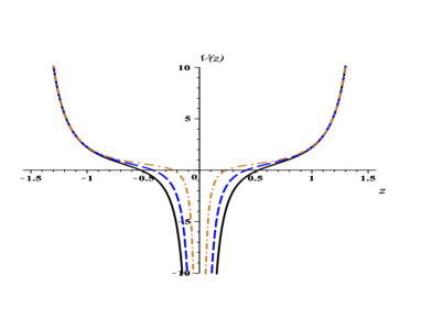
Figure 1: The effective potential $\mathcal{V}_{(-2,0)}(z)$, Eq. (14) for $\mathcal{V}_{0}=1/32$ (dot-dashed gold line), $\mathcal{V}_{0}=1/8$ (dashed blue line), and $\mathcal{V}_{0}=1/4$ (solid black line).

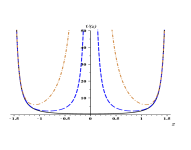
Figure 2: The effective potential $\mathcal{V}_{(-2,0)}(z)$, Eq. (14) for $\mathcal{V}_{0}=-10$ (dot-dashed gold line), $\mathcal{V}_{0}=-1$ (dashed blue line), and $\mathcal{V}_{0}=0$ (solid black line). Notice the double-well shape in z-space. The transition case $\mathcal{V}_{0}=0$ is the z-space single-well analyzed in Sec.III.1.

For an ansatz solution of the form

$$\varphi(z)=\sin^{\mu}\!(z)\cos^{\nu}\!(z)\,F(z)$$ (42)

the z-space Schrödinger equation leads to

$$F^{\prime\prime}(z)+2\left(\mu\cot\!z-\nu\tan\!z\right)F^{\prime}(z)+\left[(\mu^{2}-\mu+\mathcal{V}_{0})\cot^{2}\!z-\mu-\nu-2\mu\nu+(\nu^{2}-\nu-{}^{3}\!/{}_{\!4})\tan^{2}\!z+\mathcal{E}-{}^{1}\!/{}_{\!2}\right]F(z)=0,$$ (43)

which, by choosing

$$\mu = \frac{1}{2}\pm\frac{1}{2}\sqrt{1-4\mathcal{V}_{0}}$$ (44)

$$\nu = \pm\frac{3}{2},$$ (45)

can be written as

$$F^{\prime\prime}(z)+2\left(\mu\cot\!z-\nu\tan\!z\right)F^{\prime}(z)+\left(\mathcal{E}-{}^{1}\!/{}_{\!2}-\mu-\nu-2\mu\nu\right)F(z)=0,$$ (46)

Now, further changing variables the definition of $\xi=\sin^{2}\!z$ yields

$$\xi(1-\xi)F^{\prime\prime}(\xi)+\left(\mu+{}^{1}\!/{}_{\!2}-(1+\mu+\nu)\,\xi\right)\,F^{\prime}(\xi)+{}^{1}\!/{}_{\!4}\left(\mathcal{E}-{}^{1}\!/{}_{\!2}-\mu-\nu-2\mu\nu\right)F(\xi)=0,$$ (47)

which can be recognized as a Gauss hypergeometric equation. Its linearly independent solutions are the hypergeometric series ${}_{2}F_{1}(a,b;c;\xi)$ and $\xi^{1-c}{}_{2}F_{1}(a-c+1,b-c+1;2-c;\xi)$ (for $c\neq 1$) abramowitz . In our case, the parameters have the following values

$$a = \frac{\mu}{2}+\frac{\nu}{2}-\frac{1}{2}\sqrt{\mathcal{E}+{}^{1}\!/{}_{\!4}-\mathcal{V}_{0}}$$ (48)

$$b = \frac{\mu}{2}+\frac{\nu}{2}+\frac{1}{2}\sqrt{\mathcal{E}+{}^{1}\!/{}_{\!4}-\mathcal{V}_{0}}$$ (49)

$$c = \mu+\frac{1}{2}.$$ (50)

Solutions to the $(p,q)=(-2,0)$ Schrödinger Eq. (13) therefore read

$$\varphi^{(1)}(z) = \sin^{\mu}\!z\cos^{\nu}\!z\,{}_{2}F_{1}(a,b;c;\sin^{2}\!z)$$ (51)

$$\varphi^{(2)}(z) = \sin^{\mu}\!z\cos^{\nu}\!z\,(\sin^{2}\!z)^{1-c}{}_{2}F_{1}(a-c+1,b-c+1;2-c;\sin^{2}\!z).$$ (52)

In order to cut the hypergeometric series we must compel respectively $a=-n$ and $a-c+1=-n$ with $n\,\epsilon\,N$. This is because ${}_{2}F_{1}(a,b;c;\xi)$ and ${}_{2}F_{1}(a-c+1,b-c+1;2-c;\xi)$ diverge for $\xi=1$ while boundary conditions impose $\varphi(z=\pm\pi/2)=0$ in both cases. Note also that due to $\cos^{\nu}\!z$, for a negative $\nu$ the solutions also diverge at the boundary so we set $\nu=3/2$. Now, using Eqs.(44) and (45), we analytically obtain the Eqs. (51) and (52) spectra

$$\mathcal{E}_{n}=4(n+1)\left((n+1)\pm\sqrt{{}^{1}\!/{}_{\!4}-\mathcal{V}_{0}}\right),\ \ \ \ n=0,1,2\dots$$ (53)

which are real for $\mathcal{V}_{0}\leqslant{}^{1}\!/{}_{\!4}$. However, assuming $\mu_{+}=\frac{1}{2}+\frac{1}{2}\sqrt{1-4\mathcal{V}_{0}}$, when $0<\mathcal{V}_{0}\leqslant{}^{1}\!/{}_{\!4}$ the second solution is not physically acceptable for its derivative is divergent at the origin, and when $\mathcal{V}_{0}<0$ the function itself is divergent at $z=0$. As a result, we shall discard this solution. Therefore, the physical spectrum corresponds to the ⁺ case in Eq. (53) and the energy eigenvalues are all positive. Now, for $\mu_{-}=\frac{1}{2}-\frac{1}{2}\sqrt{1-4\mathcal{V}_{0}}$ the same issues take place with the first solution and we must keep the second one. But then, the $\pm$ spectra are interchanged. In fact, the second solution with $\mu_{-}$ happens to coincide with the first solution with $\mu_{+}$ so we can consider just $\varphi^{(1)}$ with $\mu_{+}$.

Thus, in $x$-space the solutions are eventually

$$\psi_{\rm phys}(x)=\tanh^{\mu_{+}}(x)\operatorname{sech}^{2}(x){}_{2}F_{1}(a_{+},b_{+};c_{+};\tanh^{2}(x)),$$ (54)

whose probability densities are shown in Figs. 3 and 4 for the low eigenvalues. As above explained, neither the second expression, $\psi^{(2)}(x)=\tanh^{1-\mu}\!(x)\operatorname{sech}^{\nu+\frac{1}{2}}\!(x)\,{}_{2}F_{1}(a-c+1,b-c+1;2-c;\,\tanh^{2}\!(x))$, nor any of its Kummer’s transformations maier192 are physically acceptable so we shall not consider these solutions.

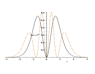
Figure 3: Plot of the normalized $|\psi_{\rm phys}(x)|^{2}$, Eq. (54), when $\mathcal{V}_{0}=1/32$ for $n=0$ (solid) $\mathcal{E}_{0}=5.8708$, $n=1$ (dashed) $\mathcal{E}_{1}=19.7417$. See in Fig. 1 the single-well effective potential $\mathcal{V}_{(-2,0)}(z)$.

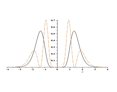
Figure 4: Plot of the normalized $|\psi_{\rm phys}(x)|^{2}$, Eq. (54), when $\mathcal{V}_{0}=-32$ for $n=0$ (solid) $\mathcal{E}_{0}=26.7156$, $n=1$ (dashed) $\mathcal{E}_{1}=61.4313$. See in Fig. 2 the double-well effective potential $\mathcal{V}_{(-2,0)}(z)$.

For $\mathcal{V}_{0}<0$ the effective potential is a double-well with a thin infinite barrier, see Fig. 2. The $z$-space solution $\varphi^{(1)}(z)$ exhibits a dumping shape about the origin, as expected for the physical solutions of an ordinary Schrödinger equation. This same behavior is transferred to the $x$-space solution as shown in Fig. 4. The energy eigenvalues are higher than the $\mathcal{V}_{0}>0$ funnel-potentials ones, and the higher they are the thinner is the dumping, as expected.

III.3 The case $(p,q)=(0,2)$, $V_{(p,q)}(x)=-V_{0}\operatorname{sech}^{2}x\,$

This case is particularly appealing because the regular constant mass Schrödinger equation is known as the Poschl-Teller equation poschlteller . The regular Poschl-Teller potential $V_{{(0,2)}}(x)=-V_{0}\operatorname{sech}^{2}x$ looks like a soft finite single-well whose bound state solutions are just associate Legendre polynomials $P_{n}^{\mu}(\tanh x),\,\mu=n,n-1,\dots 1$. On the other hand, the effective z-space potential of the PDM Poschl-Teller problem reads

$$\mathcal{V}_{{(0,2)}}(z)=\frac{1}{2}+\frac{3}{4}\tan^{2}\!z-\mathcal{V}_{0}\cos^{2}\!z,$$ (55)

and can be seen in Fig. 5 for different values of $\mathcal{V}_{0}$. Note the variation of the effective z-space potential from a single-well to a double-well when $\mathcal{V}_{0}$ crosses the -3/4 value.

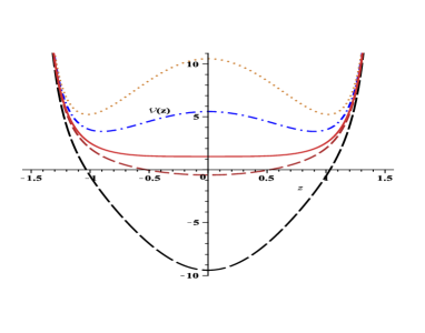
Figure 5: Plot of $\mathcal{V}_{{(0,2)}}(z)$, Eq. (55), when $\mathcal{V}_{0}=$ -10 (dotted line), -5 (dot-dashed), -3/4 (solid), 1 (dashed) and 10 (long-dashed).

In order to solve the corresponding Schrödinger equation

$$-\frac{d^{2}\varphi(z)}{dz^{2}}+\left[\frac{1}{2}+\frac{3}{4}\tan^{2}\!z-\mathcal{V}_{0}\cos^{2}\!z\right]\varphi(z)=\mathcal{E}\varphi(z),$$ (56)

we define $\varphi=\cos^{\mu}\!zH(z)$ so that we get an equation for $H(z)$

$$H^{\prime\prime}(z)-2\mu\tan(z)H^{\prime}(z)+\left(\left(\mu^{2}-\mu-{}^{3}\!/{}_{\!4}\right)\tan^{2}\!z+\mathcal{E}-\mu-{}^{1}\!/{}_{\!2}+\mathcal{V}_{0}\cos^{2}\!z\right]H(z)=0.$$ (57)

Upon a change of variables $\xi=\sin^{2}\!z$ and choosing $\mu={}^{3}\!/{}_{\!2}$ it results

$$H^{\prime\prime}(\xi)+\left(\frac{{}^{1}\!/{}_{\!2}}{\xi}+\frac{2}{\xi-1}\right)H^{\prime}(\xi)+\frac{1}{\xi(\xi-1)}\left(-\frac{\mathcal{E}}{4}+\frac{1}{2}-\frac{\mathcal{V}_{0}}{4}+\frac{\mathcal{V}_{0}}{4}\xi\right)H(\xi)=0.$$ (58)

Its solutions are therefore confluent Heun functions

$$H^{(1)}(\xi)=Hc\!\left(0,-\frac{1}{2},1,\frac{\mathcal{V}_{0}}{4},\frac{1}{2}-\frac{\mathcal{E}+\mathcal{V}_{0}}{4};\xi\right)$$ (59)

$$H^{(2)}(\xi)=\xi^{{}^{1}\!/{}_{\!2}}Hc\!\left(0,\frac{1}{2},1,\frac{\mathcal{V}_{0}}{4},\frac{1}{2}-\frac{\mathcal{E}+\mathcal{V}_{0}}{4};\xi\right),$$ (60)

and the $z$ space solutions of Eq. (13) with potential (55) result

$$\varphi^{(1)}(z)=\cos^{\frac{3}{2}}\!z\,Hc\!\left(0,-\frac{1}{2},1,\frac{\mathcal{V}_{0}}{4},\frac{1}{2}-\frac{\mathcal{E}+\mathcal{V}_{0}}{4};\sin^{2}\!z\right)\,$$ (61)

$$\varphi^{(2)}(z)=\sin\!z\,\cos^{\frac{3}{2}}\!z\,Hc\!\left(0,\frac{1}{2},1,\frac{\mathcal{V}_{0}}{4},\frac{1}{2}-\frac{\mathcal{E}+\mathcal{V}_{0}}{4};\sin^{2}\!z\right).$$ (62)

Thus, in $x$ -space we have

$$\psi^{(1)}(x)=\operatorname{sech}^{2}\!x\,Hc\!\left(0,-\frac{1}{2},1,\frac{\mathcal{V}_{0}}{4},\frac{1}{2}-\frac{\mathcal{E}+\mathcal{V}_{0}}{4};\tanh^{2}\!x\right)$$ (63)

$$\psi^{(2)}(x)=\tanh\!x\,\operatorname{sech}^{2}\!x\,Hc\!\left(0,\frac{1}{2},1,\frac{\mathcal{V}_{0}}{4},\frac{1}{2}-\frac{\mathcal{E}+\mathcal{V}_{0}}{4};\tanh^{2}\!x\right).$$ (64)

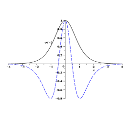
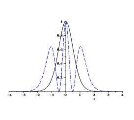
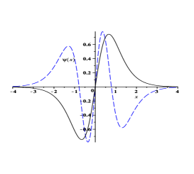
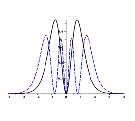
Figure 6: Plot in x-space of normalized $\psi^{(1)}(x)$ (up left) and $|\psi^{(1)}(x)|^{2}$ (up right), Eq. (63), for $\mathcal{E}_{0}=1.9749958440$ and $\mathcal{E}_{2}=11.983335512$, and $\psi^{(2)}(x)$ (down left) and $|\psi^{(2)}(x)|^{2}$ (down right), Eq. (64), for $\mathcal{E}_{1}$ = 5.982139325300; $\mathcal{E}_{3}$ = 19.9837682118. These are associated with the eigenfunctions $\varphi^{(1)}(z)$ and $\varphi^{(2)}(z)$ for a single-well potential $\mathcal{V}_{(0,2)}(z)$ with $\mathcal{V}_{0}=1/32$; this would correspond to a curve between the dashed and solid lines in Fig. 5.

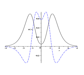
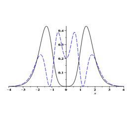
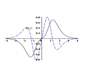
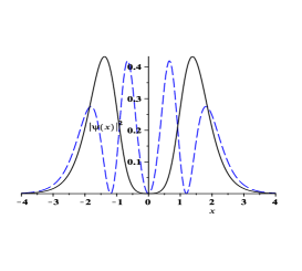
Figure 7: Plot in x-space of normalized $\psi^{(1)}(x)$ (up left) and $|\psi^{(1)}(x)|^{2}$ (up right), Eq. (63), for $\mathcal{E}_{0}$ = 26.08773401704787 and $\mathcal{E}_{2}$ = 45.5205884270, and $\psi^{(2)}(x)$ (down left) and $|\psi^{(2)}(x)|^{2}$ (down right), Eq. (64), for $\mathcal{E}_{1}$= 26.10903614483 and $\mathcal{E}_{3}$= 47.56773146428. These are associated with the eigenfunctions $\varphi^{(1)}(z)$ and $\varphi^{(2)}(z)$ for a double-well potential $\mathcal{V}_{(0,2)}(z)$ with $\mathcal{V}_{0}=-50$; this would correspond to a curve above the dotted line in Fig. 5.

It is noteworthy the fact that the PDM effect is dramatic in every aspect. For example, a potential barrier given by $V_{{(0,2)}}(x),\,V_{0}<0$, acts as an effective confining double-well potential $\mathcal{V}_{(0,2)}(z)$ once the full differential equation is considered, see Fig. 5 (dot and dot-dashed lines). The corresponding x-space wave-function behavior and probability distribution can be seen in the associated eigenstates, Eqs. (63) and (64), as shown in Fig. 7.

III.4 A special $(p,q)=(2,0)$ case, $V(x)=-V_{0}\sinh^{2}x\,$

The inverse case, $(p,q)=(2,0)$, $V(x)=-V_{0}\sinh^{2}x\,$ does not exactly belong to the family defined in Sec. II.2 (since here $p>q$) but it looks similar to its members and is also an interesting hyperbolic single-well. So, it is appropriate to briefly show its solutions here cunha-christiansen2013 . Note that $V_{(2,0)}(z)=-V_{0}\tan^{2}z$ which for the particular choice $V_{0}={3a^{2}\hbar^{2}}/{8m_{0}}$ makes ${\cal V}_{(2,0)}(z)$ trivial; see Eq. (14). The exact solutions to the corresponding PDM problem can be then easily obtained

$$\varphi(z)=C_{1}\sqrt{\frac{2}{\pi}}\cos\big{[}(2n+1)z\big{]}+C_{2}\sqrt{\frac{2}{\pi}}\sin\left(2nz\right).$$ (65)

For vanishing boundary conditions at $z=\pm\pi/2$, the energy is quantized as

$$\mathcal{E}=\frac{a^{2}\hbar^{2}\pi^{2}}{8m_{0}}n^{2}$$ (66)

where $n\in\mathbb{N}$. In $x$ space we obtain, from Eqs. (65) and (10),

$$\psi(x)=C_{1}\sqrt{\frac{2}{\pi}}\operatorname{sech}^{1/2}\!x\,\operatorname{sech}\big{[}(2n+1)x\big{]}+C_{2}\sqrt{\frac{2}{\pi}}\operatorname{sech}^{1/2}\!x\,\tanh(2nx).$$ (67)

III.5 The case $(p,q)=(2,4)$, $V_{(2,4)}(x)=-V_{0}\sinh^{2}x\operatorname{sech}^{4}x\,$

This potential, $V_{(2,4)}=-V_{0}\sinh^{2}x\operatorname{sech}^{4}x\,$ (see Fig. 8), for ${V}_{0}>0$ represents a double-well in x-space regardless of the mass dependence.

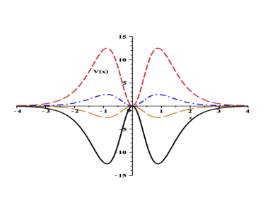
Figure 8: Plot of ${V}_{{(2,4)}}(x)$ when ${V}_{0}=$ 50 (solid black line), 10 (dashed gold), -10 (dot-dashed blue), -50 (dashed red).

The z-space effective potential for the corresponding ordinary Schrödinger equation (13) results

$$\mathcal{V}_{{(0,2)}}(z)=\frac{1}{2}+\frac{3}{4}\tan^{2}\!z-\mathcal{V}_{0}\sin^{2}\!z\cos^{2}\!z.$$ (68)

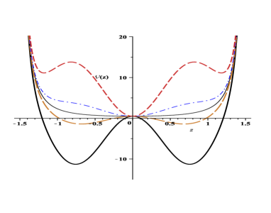
Figure 9: Plot of $\mathcal{V}_{{(2,4)}}(z)$, Eq. (68), when $\mathcal{V}_{0}=$ 50 (solid black line), 10 (dashed gold), -10 (dot-dashed blue), -50 (dashed red) associated with Fig. 8.

By defining $\xi=\sin^{2}\!z$, Eq. (13) becomes

$$\xi(\xi-1)\varphi^{\prime\prime}(\xi)+\left(\xi-\frac{1}{2}\right)\varphi^{\prime}(\xi)-\frac{1}{4}\left(\mathcal{E}-\frac{1}{2}+\frac{3}{4}\frac{\xi}{\xi-1}-\mathcal{V}_{0}\xi(\xi-1)\right)\varphi(\xi)=0,$$ (69)

which by means of

$$\varphi(\xi)=(1-\xi)^{\mu}e^{\nu\xi}h(\xi)$$

gives the following differential equation for $h(\xi)$

$$h^{\prime\prime}(\xi)+\left(2\nu+\frac{2\mu+{}^{1}\!/{}_{\!2}}{\xi-1}+\frac{{}^{1}\!/{}_{\!2}}{\xi}\right)h^{\prime}(\xi)+\frac{1}{\xi(\xi-1)}+\left(-\frac{\mathcal{E}}{4}+\frac{1}{8}+\frac{\mu-\nu}{2}+\nu(1+2\mu)\xi\right)h(\xi)=0,$$ (70)

provided

$$\mu^{2}-\frac{\mu}{2}-\frac{3}{16}=0,\ \ \ \ \nu^{2}+\frac{\mathcal{V}_{0}}{4}=0.$$

The general solution to Eq. (70) is given by the following confluent Heun functions

$$h(\xi)=A_{1}\,Hc\!\left(2\nu,\,-\frac{1}{2},\,2\mu-\frac{1}{2},\,0,\,\frac{1}{2}-\frac{\mathcal{E}}{4};\,\xi\right)+A_{2}\,\xi^{{}^{1}\!/{}_{\!2}}Hc\!\left(2\nu,\,\frac{1}{2},\,2\mu-\frac{1}{2},\,0,\,\frac{1}{2}-\frac{\mathcal{E}}{4};\,\xi\right).$$ (71)

The L.I. physical solutions are found for $\mu=\frac{3}{4}$ and $\nu=-\frac{\sqrt{-\mathcal{V}_{0}}}{2}$, resulting in

$$\varphi^{(1)}(z)=\,\cos^{\frac{3}{2}}\!ze^{-\frac{1}{2}\sqrt{-\mathcal{V}_{0}}\sin^{2}\!z}Hc\!\left(-\sqrt{-\mathcal{V}_{0}},\,-\frac{1}{2},\,1,\,0,\,\frac{1}{2}-\frac{\mathcal{E}}{4};\,\sin^{2}\!z\right)$$ (72)

$$\varphi^{(2)}(z)=\,\cos^{\frac{3}{2}}\!z\,e^{-\frac{1}{2}\sqrt{-\mathcal{V}_{0}}\sin^{2}\!z}\,\sin\!z\,Hc\!\left(-\sqrt{-\mathcal{V}_{0}},\,\frac{1}{2},\,1,\,0,\,\frac{1}{2}-\frac{\mathcal{E}}{4};\,\sin^{2}\!z\right),$$ (73)

which in $x$-space read (see Figs. 10 and 11)

$$\psi^{(1)}(x)=A_{1}\,\operatorname{sech}^{2}\!x\,e^{-\frac{1}{2}\sqrt{-\mathcal{V}_{0}}\tanh^{2}\!x}Hc\!\left(-\sqrt{-\mathcal{V}_{0}},\,-\frac{1}{2},\,1,\,0,\,\frac{1}{2}-\frac{\mathcal{E}}{4};\,\tanh^{2}\!x\right)$$ (74)

$$\psi^{(2)}(x)=A_{2}\,\operatorname{sech}^{2}\!x\,e^{-\frac{1}{2}\sqrt{-\mathcal{V}_{0}}\tanh^{2}\!x}\,\tanh\!x\,Hc\!\left(-\sqrt{-\mathcal{V}_{0}},\,\frac{1}{2},\,1,\,0,\,\frac{1}{2}-\frac{\mathcal{E}}{4};\,\tanh^{2}\!x\right).$$ (75)

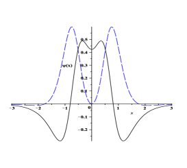
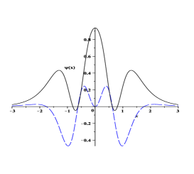
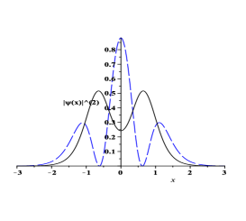
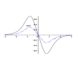
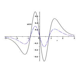
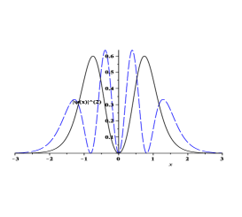
Figure 10: Plot in x-space of normalized real (solid line) and imaginary (dashed) parts of $\psi^{(1)}(x)$, Eq. (74), for $\mathcal{E}_{0}=-5.210246244135$ (up left), $\mathcal{E}_{2}=5.7464269736389$ (up center), and $|\psi^{(1)}(x)|^{2}$ for both energies (up right), and real (solid line) and imaginary (dashed) parts of $\psi^{(2)}(x)$, Eq. (75), for $\mathcal{E}_{1}$= -3.793253878015 (down left) and $\mathcal{E}_{3}$= 13.0906628480 (down center) and $|\psi^{(2)}(x)|^{2}$ (down right) for both energies. These correspond to the eigenfunctions $\varphi^{(1)}(z)$ and $\varphi^{(2)}(z)$ for a double-well potential $\mathcal{V}_{(2,4)}(z)$ when $\mathcal{V}_{0}=50$; see Fig. 9.

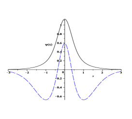
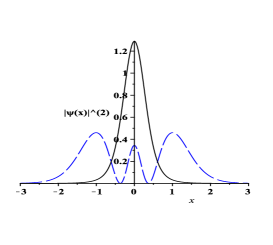
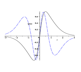
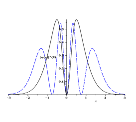
Figure 11: Plot in x-space of normalized $\psi^{(1)}(x)$ (up left) and $|\psi^{(1)}(x)|^{2}$ (up right), Eq. (74), for $\mathcal{E}_{0}$ = 6.46273117442 (solid line), $\mathcal{E}_{2}$ = 20.09128324147 (dashed), and $\psi^{(2)}(x)$ (down left) and $|\psi^{(2)}(x)|^{2}$ (down right), Eq. (75), for $\mathcal{E}_{1}$= 15.1770345117 (solid line) and $\mathcal{E}_{3}$= 26.7184553916 (dashed). These correspond to the eigenfunctions $\varphi^{(1)}(z)$ and $\varphi^{(2)}(z)$ for a triple-well potential $\mathcal{V}_{(2,4)}(z)$ when $\mathcal{V}_{0}=-50$; see Fig. 9.

An analytical survey indicates that the effective z-space potentials vary from double-wells (for $\mathcal{V}_{0}>3/4$), pass through single-wells (for $-81/4<\mathcal{V}_{0}<3/4$), and then to triple-wells (for $-81/4>\mathcal{V}_{0}$); see Fig. 9. The x-space eigenfunctions exhibit the corresponding behavior, similar to the z-shape, as shown by the probability densities displayed in Figs. 10, 11 and 12. We could not find a cut for the series in the present case so energy eigenvalues have been computed numerically.

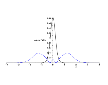
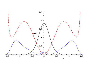
Figure 12: (left) Plot of normalized $|\psi^{(1)}(x)|^{2}$ in x-space, Eq. (74), corresponding to the eigenfunctions plotted at the right. (right) Plot of $\mathcal{V}_{{(2,4)}}(z)$ (dot-dashed red line) and $|\varphi^{(1)}(z)|^{2}$ for $\mathcal{E}_{0}=11.675703293036$ (solid black) and $\mathcal{E}_{2}=37.459017784502$ (dashed blue), when $\mathcal{V}_{0}=-150$.

IV Final Remarks

We have analyzed, in the framework of position-dependent massive quantum particles, a recently reported family of hyperbolic potentials downing . In the context of the ordinary constant mass Schrödinger equation, the author of downing signaled the role of the confluent Heun functions in the dynamics of two family members, emphasizing the fact that Heun functions are rather exotic though increasingly popular in contemporary physics and mathematics. Indeed, Heun functions have been practically absent in the literature for almost one century but have been lastly emerging in all frontiers of physics christiansencunha2011 ; christiansencunha2012 ; rumania ; bulgaria ; cvetic2011 ; herzog . In the present paper, we reconsidered the same class of potentials when the mass is promoted to a phenomenologically interesting soliton-like distribution. We extended the number of cases analyzed so that our results are rather comprehensive. Although the differential equations are dramatically modified, we managed to analytically handle them and found their solutions in several cases. In fact, the PDM upgrade makes the equations much more difficult and some family members have no analytical solutions for PDM, e.g. the cases $q=4,6$ which for a constant mass have confluent Heun solutions. Among the soluble members in the PDM framework, we have identified confluent Heun solutions in most of them. For example, the cases $(-2,2)$, $(0,2)$ and $(2,2)$ have hypergeometric solutions for a constant mass but become confluent Heun functions for PDM. We also worked out the PDM Poschl-Teller potentials and the PDM hyperbolic double-well for their phenomenological relevance and found both to have confluent Heun solutions. Finally, we would like to point the fact that analogue cases belonging to a larger class which admits odd parameters $p$ and $q$ can also have Heun solutions. For example, in the case $V_{(1,1)}(x)=-V_{0}\tanh\!x$, which corresponds to $\mathcal{V}(z)=\frac{1}{2}+\frac{3}{4}\tan^{2}(z)-\mathcal{V}_{0}\sin(z)$, solutions read cunha-christiansen2013 $\psi(x)=\left({{}^{1}\!/{}_{\!2}+{}^{1}\!/{}_{\!2}\tanh{x}}\right)\,Hc(0,1,-1,2\mathcal{V}_{0},{}^{1}\!/{}_{\!2}-\mathcal{V}_{0}-\mathcal{E};{}^{1}\!/{}_{\!2}+{}^{1}\!/{}_{\!2}\tanh{x}).$

References

- (1) C. Cohen-Tannoudji, B. Diu, F. Laloë, Mécanique Quantique, Ed. Hermann, Paris 1977.
- (2) P. M. Morse, Phys. Rev. 34 (1929) 57.
- (3) C. Eckart, Phys. Rev. 35 (1930) 1303.
- (4) N. Rosen and P. M. Morse, Phys. Rev. 42 (1932) 210.
- (5) M. F. Manning and N. Rosen, Phys. Rev. 44 (1933) 953.
- (6) G. Pöschl, E. Teller, Zeitschrift für Physik 83 (1933) 143.
- (7) M. F. Manning, J. Chem. Phys. 3 (1935) 136; Phys. Rev. 48 (1935) 161.
- (8) S.T. Ma, Phys. Rev. 71 (1947) 195.
- (9) V. Bargmann, Rev. Mod. Phys. 21 (1949) 488.
- (10) F. Scarf, Phys. Rev. 112 (1958) 1137.
- (11) H. Fiedeley, W.E. Frahn, Ann. Phys. (N.Y.) 16 (1961) 387
- (12) A. Bhattacharjie, E.C.G. Sudarshan, Nuovo Cim. 25 (1962), 864
- (13) A. K. Bose, Nuovo Cim. 32 (1964) 679.
- (14) G. Bencze, Comm. Phys. Math. 31 (1966) 1.
- (15) G. A. Natanzon, Teoret. Mat. Fiz. 38 (1979) 146.
- (16) M. M. Nieto, Phys. Rev. A 17 (1978) 1273.
- (17) Y. Alhassid, F. Gürsey, F. Iachello, Phys. Rev. Lett. 50 (1983) 873.
- (18) J. N Ginocchio, Ann. Phys (NY) 152 (1984) 203.
- (19) A. Arda, R. Sever, Comm. Theor. Phys. 56, 51 (2011).
- (20) H. Panahiy, Z. Bakhshi, Acta Phys. Pol. B 41 (2010) 11.
- (21) R. Sever, C. Tezcan , Int. J. of Mod. Phys. E 17 (2008) 1327.
- (22) B. Midya, Barnana Roy, Phys. Lett. A 373 (2009) 4117.
- (23) B. Bagchi, P. Gorain, C. Quesne, R. Roychoudhury, Mod. Phys. Lett. A 19 (2004) 2765.
- (24) G. H. Wannier, Phys. Rev. 52 (1937) 191.
- (25) J. C. Slater, Phys. Rev. 76 (1949) 1592.
- (26) M. Luttinger, W. Kohn, Phys. Rev. 97 (1955) 869.
- (27) G. Bastard, Phys. Rev. B 24 (1981) 5693.
- (28) O. von Roos, Phys. Rev. B 27 (1983) 7547.
- (29) G. T. Einevoll and P. C. Hemmer, J. Phys. C 21 (1988) L1193.
- (30) J.-M. L vy-Leblond, Phys. Rev. A 52 (1995) 1845.
- (31) D. J. Ben-Daniel and C. B. Duke, Phys. Rev. 152 (1966) 683.
- (32) Qi-G. Zhu and H. Kroemer, Phys. Rev. B 27, (1983) 3519 3527 .
- (33) C. Weisbuck and B. Vinter, Quantum Semiconductor Structures Academic, Boston, 1991.
- (34) T. Gora and F. Williams, Phys. Rev. 177 (1969) 1179.
- (35) G. Bastard, J. K. Furdyna, J. Mycielsky, Phys. Rev. B 12 (1975) 4356.
- (36) G. Bastard, Wave Mechanics Applied to Semiconductor Heterostructure Editions de Physique, Les Ulis, 1988; G. Levai, J. Phys. A: Math. Gen. 27 (1994) 3809.
- (37) P. Harrison, Quantum Wells, Wires and Dots Wiley, New York, 2000; L. Serra and E. Lipparini, Europhys. Lett. 40 (1997) 667.
- (38) M. Barranco, M. Pi, S. M. Gatica, E. S. Hernandez, and J. Navarro, Phys. Rev. B56 (1997) 8997.
- (39) M. R. Geller and W. Kohn, Phys. Rev. Lett. 70 (1993) 3103.
- (40) F. Arias de Saavedra, J. Boronat, A. Polls, and A. Fabrocini; Phys. Rev. B50 (1994) 4248.
- (41) M. Willatzen, B. Lassen, J. Phys.: Cond. Matter 19 (2007) 136217.
- (42) C. A. Downing, J. Math. Phys. 54 (2013) 072101.
- (43) M. Abramowitz and I. Stegun, Handbook of Mathematical Functions Dover, New York, 1972.
- (44) K. Heun, Math. Ann. 33 (1889) 161.
- (45) A. Ronveaux, Heun’s differential equations, Oxford University Press Oxford 1995.
- (46) R. S. Maier, Math. J. of Computation 76, n. 258, (2007) 811.
- (47) A. Decarreau, P. Maroni, A. Robert, Ann. Soc. Sci Brux. T92(III) 151 (1978).
- (48) R. S. Maier, J. Diff. Equations 213, (2005) 171.
- (49) E. Hille, Ordinary Differential Equations in the Complex Domain, 1.ed. Dover Science, New York 1997.
- (50) S. Y. Slavyanov and W. Lay Special Functions: A Unified Theory Based on Singularities Mathematical Monographs, Oxford 2000.
- (51) M. N. Hounkonnou, A. Ronveaux, App. Math. Comp. 209 (2009) 421.
- (52) P. P. Fiziev, J. Phys. A: Math. Theor. 43 (2010) 035203.
- (53) J. R. Shewell, Am. J. Phys. 27 (1959) 16.
- (54) R. A. Morrow and K. R. Brownstein, Phys. Rev. B 30 (1984) 678.
- (55) O. Von Roos and H. Mavromatis, Phys. Rev. B 31 (1985) 2294.
- (56) R. A. Morrow, Phys. Rev.B 36 (1987) 4836; Phys. Rev. B 35 (1987) 8074.
- (57) I. Galbraith, G. Duggan, Phys. Rev. B 38 (1988) 057.
- (58) T. Li, K.J. Kuhn, Phys. Rev. B 47 (1993) 12760.
- (59) J. Thomsen, G. T. Einevoll, P. C. Hemmer, Phys. Rev. B 39 (1989) 783.
- (60) K. Young, Phys. Rev. B 39 (1989) 434.
- (61) G. T. Einevoll, Phys. Rev. B 42 (1990) 3497.
- (62) G. T. Einevoll, P. C. Hemmer, and J. Thomsen, Phys. Rev. B 42 (1990) 3485.
- (63) T.D. Lee, Particle Physics and Introduction to Field Theory. Harwood Academic Publishers, Newark 1981.
- (64) A. de Souza Dutra, C. A. Almeida, Phys. Lett. A 275 (2000) 25.
- (65) M. S. Cunha, H. R. Christiansen, Commun. Theor. Phys. 60 (2013) 642. arXiv:1306.0933.
- (66) M. S. Cunha, H. R. Christiansen, Phys. Rev. D 84 (2011) 085002.
- (67) H. R. Christiansen, M. S. Cunha, Eur. Phys. J. C 72 (2012) 1942.
- (68) M.A. Dariescu, C. Dariescu, Astrophys. Space Sci. 341 (2012) 429.
- (69) P. Fiziev, D. Staicova, Phys. Rev. D 84 (2011) 127502.
- (70) T. Birkandan, M. Cvetic, Phys. Rev. D 84 (2011) 044018.
- (71) C. P. Herzog, Jie Renb, J. High En. Phys. 1206 (2012) 078.