Twisted reduction in large N QCD with adjoint Wilson fermions

Abstract:

The twisted space-time reduced model of large $N$ QCD with various flavours of adjoint Wilson fermions is constructed applying the symmetric twist boundary conditions with flux $k$. The models with one and two flavours show distinctive behaviours. For the two flavor case, the string tension, calculated at $N=289$, approaches zero as we decrease the quark mass in a way consistent with the theory being governed by an infrared fixed point. In contrast, the string tension for the case of a single adjoint Wilson fermion remains finite as the quark mass decreases to zero, supporting that this is a confining theory.

1 Introduction

The dynamics of SU($N$) gauge theories with adjoint fermions is expected to depend crucially on the number of flavors $N_{f}$. This is suggested by inspecting the $N_{f}$ dependence of the beta function $\beta$. The first two coefficients of $\beta$ expressed in terms of ’t Hooft coupling $\lambda=g^{2}N$ are $b_{0}=(4N_{f}-11)/24\pi^{2}$ and $b_{1}=(16N_{f}-17)/192\pi^{4}$. Asymptotic freedom requires that $b_{0}$ should be negative, so only $N_{f}$=1 and 2 are allowed (in this talk we do not consider half-integer $N_{f}$ corresponding to Majorana fermions). For $N_{f}$=1, $b_{1}$ is also negative, so we naturally expect that the theory is confining as ordinary QCD. For $N_{f}$=2, on the contrary, $b_{1}$ is positive, indicating that there could be an infrared fixed point at finite value of the ’t Hooft coupling where the beta function becomes zero. Since no dimensional scale exists at the infrared fixed point, this theory is conjectured to be conformal. In fact, for $N$=2 (minimal walking technicolor), there are now many lattice simulations indicating that the theory is conformal at vanishing fermion mass[1].

The purpose of the present talk is to study both $N_{f}$=1 and 2 theories in the large $N$ limit. It is quite obvious that the direct application of the usual lattice simulation is unpractical for large $N$. Our idea is to use the twisted space-time reduced model defined on a $1^{4}$ lattice, recently proposed by the present authors[2]. We point out that, in recent years, many authors have studied space-time reduced models of large $N$ QCD with adjoint fermions using periodic boundary conditions[3, 4, 5, 6]. It turns out, however, that these models have too large finite $N$ corrections compared with those based on twisted boundary conditions[2, 4], casting doubts on whether the former models are of practical use. The main finite $N$ corrections of the twisted reduced model for $N=L^{2}$ amount to the finite volume corrections of ordinary Lattice Gauge Theory on an $L^{4}$ lattice[2, 7]. Thus, by choosing $N=17^{2}=289$, we can study large $N$ QCD with adjoint fermions on an effectively $17^{4}$ lattice within the present computer resources. From a practical point of view, the most important property of the reduced model is its rather small memory size. In fact, the size of four SU(289) matrices is only 5 MB, which can be fitted into cache memory, resulting in a rather high performance of computations. By making use of these advantages of the reduced model, we will analyze the properties of large $N$ QCD with adjoint fermions and clarify the difference of $N_{f}$=1 and 2 fermions.

2 Formulation

We consider the SU($N$) group with $N=L^{2}$, $L$ being some positive integer. Then the action of the twisted space-time reduced model of QCD with $N_{f}$ adjoint fermions is given by[2]

$$S = -bN\sum_{\mu\neq\nu=1}^{4}{\rm Tr}\left[z_{\mu\nu}U_{\mu}U_{\nu}U_{\mu}^{\dagger}U_{\nu}^{\dagger}\right]$$ (1)

$$-\sum_{j=1}^{N_{f}}{\rm Tr}\left[\right.{\bar{\Psi}}^{j}\Psi^{j}-\kappa\sum_{\mu=1}^{4}\left\{{\bar{\Psi}}^{j}(1-\gamma_{\mu})U_{\mu}\Psi^{j}U_{\mu}^{\dagger}+{\bar{\Psi}}^{j}(1+\gamma_{\mu})U_{\mu}^{\dagger}\Psi^{j}U_{\mu}\right\}\left.\right]$$

$$\equiv -bN\sum_{\mu\neq\nu=1}^{4}{\rm Tr}\left[z_{\mu\nu}U_{\mu}U_{\nu}U_{\mu}^{\dagger}U_{\nu}^{\dagger}\right]-2\kappa\sum_{j=1}^{N_{f}}{\rm Tr}\left[{\bar{\Psi}}^{j}D_{W}\Psi^{j}\right].$$

$U_{\mu}$ are four SU($N$) link variables and $\Psi^{j}$ are $N_{f}$ Grassman-valued $N\times N$ matrices transforming in the ($N,{\bar{N}}$) color representation. Spinor indices of $\Psi^{j}$ are not explicitly shown. $b$ is the inverse (lattice) ’t Hooft coupling $b=1/g^{2}N$ and $\kappa$ is the hopping parameter of Wilson fermions. The symmetric twist tensor $z_{\mu\nu}$ is an element of Z($L$), whose explicit form is

$$z_{\mu\nu}=\exp\left(k{2\pi i\over L}\right),\ \ \ z_{\nu\mu}=z_{\mu\nu}^{*},\ \ \ \mu>\nu$$ (2)

The integer $k$ represents the flux through each plane. $k$ and $L$ should be co-prime, and a general prescription for choosing $k$ and $L$ to minimize the finite $N$ corrections is given in Ref. [2]. The condition is essentially the same as the one imposed in the pure gauge model to prevent Z($L$) symmetry breaking[8], which is necessary for reduction to work[9, 10]. We recall that our prescription is to take both $k/L$ and $\bar{k}/L$ (defined $k\bar{k}=1$ mod $L$) large enough. Throughout this paper we use $L$=17 ($N=L^{2}=289$), $k$=5, and thus $\bar{k}$=7. We have studied the model with $N_{f}=2$ by means of the Hybrid Monte Carlo method. For $N_{f}=1$, we have used the Rational Hybrid Monte Carlo method.

Simulations have been done at two values of the inverse ’t Hooft coupling $b$ = 0.35 and 0.36. For $N_{f}$=2, we have made simulations at eight values of $\kappa$ = 0.05, 0.10, 0.11, 0.12, 0.13, 0.14, 0.15 and 0.16. For $N_{f}$=1, we attempted to make simulations at the same eight values of $\kappa$. However, we found that, for $\kappa>$ 0.155, the CG iteration during the molecular dynamics evolution does not converge. Hence, for $N_{f}$=1 we took $\kappa$ = 0.05, 0.10, 0.11, 0.12, 0.13, 0.14, 0.15 and 0.155 instead.

For every configuration we calculated the expectation value of ${\rm Tr}(U_{\mu}^{\ell}$), for $1\leq\ell\leq(L-1)$, which are the order parameters of the Z${}^{4}(L)$ symmetry. We confirm that, in all the simulations presented here, the quantities $<{\rm Tr}(U_{\mu}^{\ell})>$ are compatible with zero within statistical errors. For randomly chosen gauge configurations, we also calculated all traces of open loops within the effective $L^{4}$ box, checking that traces of all open loops are zero within statistical errors.

Figure 1: Histogram of ${1\over N}{\rm ReTr}(U_{\mu}^{L})$ for $N_{f}$=2 and $b=0.35$. (a) $\kappa$=0.15. (b) $\kappa$=0.16.

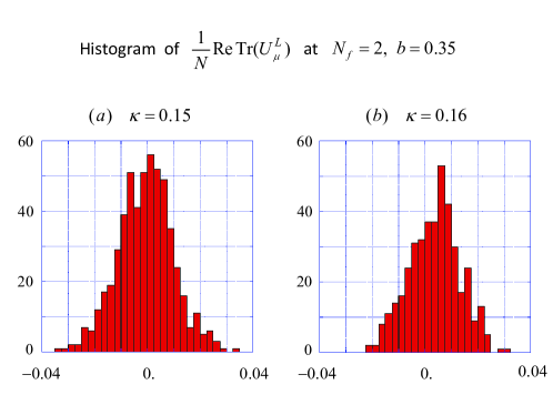
During the simulations we also calculated ${\rm Tr}(U_{\mu}^{L})$. We point out that this quantity could have a non-zero value without breaking the Z${}^{4}(L)$ symmetry of the reduced model. The association of our system with an ordinary lattice system of size $L^{4}$, indeed suggests that at sufficiently weak coupling a non-zero expectation value would be observed. However, we confirmed that $<{\rm Tr}(U_{\mu}^{L})>$ is statistically compatible with zero for all our simulations except for two runs at $N_{f}=2$ and $\kappa=0.16$. This is illustrated in Fig.1, where we display the histogram of ${1\over N}{\rm ReTr}(U_{\mu}^{L})$ at $\kappa$=0.15 and 0.16 for $b=0.35$. While the histogram is centered at ${1\over N}{\rm ReTr}(U_{\mu}^{L})$=0 for $\kappa$=0.15, it is slightly shifted towards positive values for $\kappa$=0.16. We observe the same phenomena at $b$=0.36. We expect the change of pattern to take place when a certain correlation length of the system becomes comparable to the effective size of the box $L$. Indeed, as shown in sect. 4, for $\kappa$=0.16 the dimensionless ratio $1/(L\sqrt{\sigma})$ reaches $\sim$0.6.

3 Quark mass $m_{q}$

One of the simplest quantities that one can study is the low-lying spectrum of the square of the hermitian Wilson Dirac matrix $Q^{2}=(D_{W}\gamma_{5})^{2}$. The lowest eigenvalue provides a possible definition of the quark mass as follows $m_{q}=\sqrt{\lambda}$, where we use the lattice units $a$=1. There is a small correction here since the boundary conditions prohibit zero-momentum states. Thus, the lowest eigenvalue contains a small $1/N$ correction to the mass, which we have neglected. On the other hand, the bare quark mass is given by $M_{q}^{(0)}=\frac{1}{2}(\frac{1}{\kappa}-\frac{1}{1/8})$. Renormalization implies the necessity of an additive renormalization and multiplicative renormalization of the mass. Thus, we can parametrize the dependence as follows

$$m_{q}=A\left(\frac{1}{2\kappa}-\frac{1}{2\kappa_{c}}\right)^{\delta}\left[1+B\left({1\over\kappa}-{1\over\kappa_{c}}\right)\right]$$ (3)

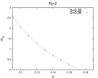
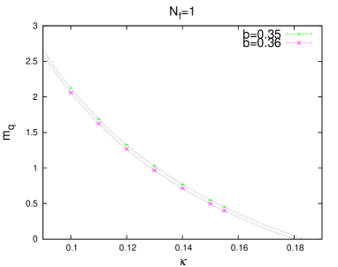
where we have included a possible $O(m_{q})$ correction since we are dealing with Wilson fermions. For a QCD-like theory one expects $\delta=1$ [11]. However, if the theory has an infrared fixed-point at $\kappa=\kappa_{c}$, the exponent could be different from 1. We have fitted our parameterization to our data in the range $\kappa=0.10-0.15$. The data at $\kappa$=0.05 is too far to neglect higher order corrections in $m_{q}$. On the other hand, we excluded $\kappa$=0.16, since in that case the system might suffer from finite size effects. The results, however, do not change significantly when including this value. Good fits are obtained at $N_{f}=2$ and the fitting parameters are $\delta=0.914(11)$, $\kappa_{c}=0.1744(3)$ at $b$=0.35, and $\delta=0.920(14)$, $\kappa_{c}=0.1722(5)$ at $b$=0.36. In both cases the $\delta=1$ value is statistically disfavored. We have repeated the same analysis for $N_{f}$=1. Here we use the data in the range $\kappa=0.10-0.155$. We get at $b$=0.35, $\delta=1.010(14)$, $\kappa_{c}=0.1834(5)$ and at $b$=0.36, $\delta=1.021(11)$, $\kappa_{c}=0.1804(3)$, compatible with the naively expected behavior $\delta$=1. Thus, we conclude that the quark mass $m_{q}$ gives evidence of a different critical behavior for $N_{f}$=2 and 1. The results for $m_{q}$ as a function of $\kappa$ for both cases are displayed in figs. 3 and 3, together with the best fit lines.

Figure 2: $\kappa$ dependence of $m_{q}$ for $N_{f}$=2.

Figure 3: $\kappa$ dependence of $m_{q}$ for $N_{f}$=1.

4 String tension

The string tension $\sigma$ is extracted from the large $R$ behavior of the square Creutz ratio $\chi(R,R)$ as follows:

$$\chi(R,T)= -\log{\frac{W(R+0.5,T+0.5)W(R-0.5,T-0.5)}{W(R+0.5,T-0.5)W(R-0.5,T+0.5)}}$$ (4)

$$\chi(R,R)\xrightarrow[R\to\infty]{}\sigma+{2\eta\over R^{2}}+{\xi\over R^{4}}+\cdots.$$

This method has been used successfully for the pure gauge theory (twisted Eguchi-Kawai model) [12], where the three parameter ($\sigma$, $\eta$ and $\xi$) formula describes the data very well. For our adjoint fermion case, the smaller effective size $L$=17 and fewer statistics limits the range of $R$ values that can be fitted to Eq. (4). This introduces strong correlations among the parameters and a rather poor determination of the $\kappa$ dependence of each parameter. A better way to proceed is to fix one of the parameters and study the evolution of the other parameters with $\kappa$ and the inverse ‘t Hooft coupling $b$. From that point view the best choice is $\eta$, since it is dimensionless and its value is connected to universal properties of an effective bosonic string theory, not expected to depend on $\kappa$ or $b$.

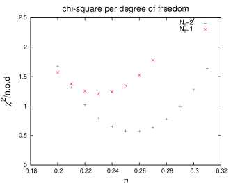
To determine the value of $\eta$ to use, we perform a simultaneous fit to all the data (with $\kappa$¿0.05) fixing the value of $\eta$ and marginalizing over the remaining parameters. The resulting chi-square profiles ($\chi^{2}/{\rm n.o.d}$) are plotted in Fig. 4 for $N_{f}$=2 and 1. The figure shows that our hypothesis of a common value of $\eta$ is statistically satisfactory. The minimum of the chi-square curve determines the best choice for $\eta$, given by $\eta$=0.26 for $N_{f}$=2 and $\eta$=0.24 for $N_{f}$=1. The curve also provides a value for the error of order $\pm(0.04-0.05)$.

Figure 4: Chi-square per degree of freedom $\chi^{2}/n.o.d$ as functions of $\eta$ both for $N_{f}$=2 and 1.

Figure 5: $m_{q}$ dependence of $\sigma$ for $N_{f}$=2 at b=0.35.

Figure 6: $m_{q}$ dependence of $\sigma$ for $N_{f}$=2 at b=0.36.

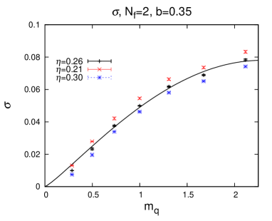
Fixing the value of $\eta$ we can obtain good fits to the Creutz ratios using the parameterization of Eq. (4). The resulting values of the string tension $\sigma$ as a function of $m_{q}$ for $N_{f}$=2 at b=0.35 are displayed in Fig. 6. The central black symbols are obtained with $\eta$=0.26, while red and blue symbols are obtained by taking $\eta$ to 0.21 and 0.30, respectively. From these values it is clear that the string tension value depends uniformly on $\eta$. The band covered between the values for $\eta$=0.21 and 0.30, serves as a rough estimate of the systematic error.

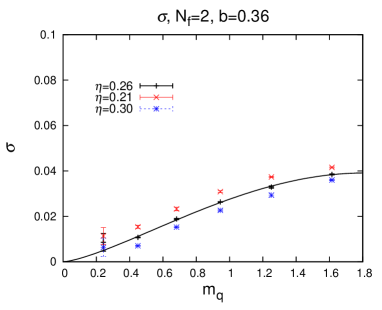
If the theory is governed by an infrared fixed point deformed with a relevant mass term $m_{q}{\bar{\Psi}}\Psi$, all physical quantities having positive mass dimensions should vanish as $m_{q}\to 0$. In particular, the string tension having dimensions of mass squared should behave as

$$\sigma=Am_{q}^{\alpha}(1+Bm_{q})$$ (5)

where we have included possible $O(m_{q})$ corrections. Our $N_{f}=2$ data are perfectly consistent with this formula as shown in Fig. 6 for $b=0.35$ and Fig. 6 for $b=0.36$. Unfortunately, the exponent $\alpha$ has a large uncertainty. A fit in the range $\kappa\in[0.10-0.15]$ for the $b=$0.35-$\eta$=0.26 data gives $\alpha=$1.17. Varying $\eta$ within the allowed range produces a systematic error of $0.12$. For the $b=$0.36-$\eta$=0.26 data one gets $\alpha=$1.42 with a systematic error of $0.25$.

Figure 7: $m_{q}$ dependence of $\sigma$ for $N_{f}$=1 at b=0.35.

Figure 8: $m_{q}$ dependence of $\sigma$ for $N_{f}$=1 at b=0.36.

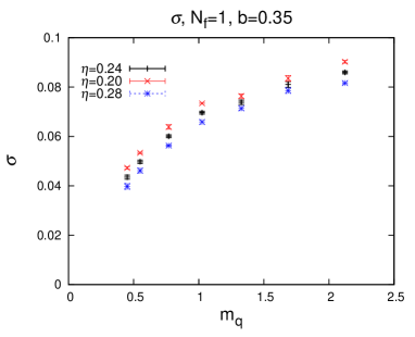
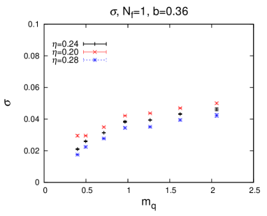
The previous results show that, for the $N_{f}=2$ case, the string tension seems to vanish at the critical point $m_{q}=0$, in accordance with the infrared fixed point hypothesis. This contrasts with the results for $N_{f}$=1, summarized in Figs. 8 and 8. The data seems to approach a non-zero value at the critical point, as expected for a QCD-like theory, with confinement and spontaneous symmetry breaking.

From the vanishing of the string tension at the critical point one can obtain a determination of the mass anomalous dimension $\gamma_{*}$ at the infrared fixed point. Equating the exponent $\alpha^{\prime}$ of $(1/\kappa-1/\kappa_{c})$ with $2/(1+\gamma_{*})$ one gets values of $\gamma_{*}=0.87$ and $0.53$ for $b=$0.35 and 0.36 respectively. The determination is dominated by the systematic error of order $\pm(0.3-0.4)$. There is no fundamental difficulty in reducing these errors significantly. As mentioned previously, an important source comes from the small effective lattice volume $L^{4}=17^{4}$ of our data. However, increasing $N=L^{2}$ poses an important challenge within the present computer power. A more promising approach follows by employing partial volume reduction [13, 14]. In particular, one can reduce the system to a $2^{4}$ lattice, which at large N should behave as living in a $(2\sqrt{N})^{4}$ box. A finer analysis of the $\kappa$ dependence close to $\kappa_{c}$ is also important. Alternatively, one can use other observables to determine $\gamma_{*}$. One possibility is to use the distribution of eigenvalues of $Q^{2}$. Some results using this method have already been presented [15].

Acknowledgments

A.G-A is supported from Spanish grants from MINECO: FPA2012-31686, FPA2012-31880, FPA2009-09017, SEV-2012-0249 and CPAN CSD2007-00042; Comunidad de Madrid: HEPHACOS S2009/ESP-1473, and European Union PITN-GA-2009-238353 (ITN STRONGnet). M. O. is supported by the Japanese MEXT grant No 23540310.

The calculation has been done on Hitachi SR16000-M1 computer at High Energy Accelerator Research Organization (KEK) supported by the Large Scale Simulation Program No.12/13-01 (FY2012-13). The authors thank the Hitachi system engineers for their help in highly optimizing the present simulation code.

References

- [1] L. Del Debbio, PoS Lattice 2010 (2010) 004; E. Neil, PoS Lattice 2011 (2011) 009; J. Giedt, PoS Lattice 2012 (2012) 006.
- [2] A. Gonzalez-Arroyo and M. Okawa, PoS Lattice 2012 (2012) 046; Phys. Rev. D 88 (2013) 014514.
- [3] P. Kovtun, M. Unsal, L. G. Yaffe, JHEP 0706 (2007) 019.
- [4] T. Azeyanagi, M. Hanada, M. Unsal, R. Yacoby, Phys. Rev. D82 (2010) 125013.
- [5] B. Bringoltz and S. R. Sharpe, Phys. Rev. D80 (2009) 065031; B. Bringoltz, M. Koren, S. R. Sharpe, Phys. Rev. D85 (2012) 094504.
- [6] A. Hietanen and R. Narayanan, JHEP 1001 (2010) 079; Phys. Lett. B698 (2011) 171.
- [7] A. Gonzalez-Arroyo and M. Okawa, Phys. Rev. D27 (1983) 2397.
- [8] A. Gonzalez-Arroyo and M. Okawa, JHEP 1007 (2010) 043.
- [9] T. Eguchi and H. Kawai, Phys. Rev. Lett. 48 (1982) 1063.
- [10] G. Bhanot, U. M. Heller and H. Neuberger, Phys. Lett. B113 (1982) 47; T. Ishikawa and M. Okawa, talk given at the Annual Meeting of the Physical Society of Japan, March 28-31, Sendai, Japan (2003); W. Bietenholz, J. Nishimura, Y. Susaki and J. Volkholz, JHEP 0610 (2006) 042; M. Teper and H. Vairinhos, Phys. Lett. B652 (2007) 359; T. Azeyanagi, M. Hanada, T. Hirata and T. Ishikawa, JHEP 0801 (2008) 025.
- [11] L. Del Debbio, L. Giusti, M. Lüscher, R. Petronzio and N. Tantalo, JHEP 0602 (2006) 011.
- [12] A. Gonzalez-Arroyo and M. Okawa, PoS Lattice 2012 (2012) 221; Phys. Lett. B718 (2013) 1524.
- [13] R. Narayanan and H. Neuberger, Phys. Rev. Lett. 91 (2003) 081601.
- [14] M. Garcia Perez, A. Gonzalez-Arroyo and M. Okawa, PoS Lattice 2012 (2012) 219; PoS Lattice 2013 (2013) 342; JHEP 1309 (2013) 003.
- [15] M. Garcia Perez, A. Gonzalez-Arroyo, L. Keegan and M. Okawa, PoS Lattice 2013 (2013) 098.