Stability boundaries and collisions of two-dimensional solitons in $\mathcal{PT}$-symmetric couplers with the cubic-quintic nonlinearity

Abstract

We introduce one- and two-dimensional (1D and 2D) models of parity-time ($\mathcal{PT}$) -symmetric couplers with the mutually balanced linear gain and loss applied to the two cores, and cubic-quintic (CQ) nonlinearity acting in each one. The 2D and 1D models may be realized in dual-core optical waveguides, in the spatiotemporal and spatial domains, respectively. Stationary solutions for $\mathcal{PT}$-symmetric solitons in these systems reduce to their counterparts in the usual coupler. The most essential problem is the stability of the solitons, which become unstable against symmetry breaking with the increase of the energy (norm), and retrieve the stability at still larger energies. The boundary value of the intercore-coupling constant, above which the solitons are completely stable, is found by means of an analytical approximation, based on the CW (zero-dimensional) counterpart of the system. The approximation demonstrates good agreement with numerical findings for the 1D and 2D solitons. Numerical results for the stability limits of the 2D solitons are obtained by means of the computation of eigenvalues for small perturbations, and verified in direct simulations. Although large parts of the solitons families are unstable, the instability is quite weak. Collisions between 2D solitons in the $\mathcal{PT}$-symmetric coupler are studied by means of simulations. Outcomes of the collisions are inelastic but not destructive, as they do not break the $\mathcal{PT}$ symmetry.

I Introduction and the setting

Wave-propagation models of physical media are naturally separated into two generic classes, conservative and dissipative. Recently, it was recognized that a more particular species of $\mathcal{PT}$ (parity-time)-symmetric systems may be identified at the boundary between these generic types Bender_review ; special-issues ; review . They are represented by dissipative quantum-mechanical models, and by classical waveguides subject to the condition of spatial antisymmetry between separated gain and loss. While in the quantum theory the $\mathcal{PT}$-symmetric models are subjects of theoretical studies, the similarity of the quantum-mechanical Schrödinger equation to the paraxial propagation equation in optics makes it possible to implement this concept in real physical settings, as proposed theoretically Muga and demonstrated experimentally experiment in a number of works. These possibilities have drawn a great deal of interest to the wave propagation in $\mathcal{PT}$-symmetric systems special-issues , especially in the presence of spatially periodic complex potentials, with even real and imaginary odd parts, as required by the $\mathcal{PT}$ symmetry PT_periodic ; review .

The ubiquitous occurrence of the Kerr nonlinearity in photonic media is an incentive for studies of nonlinear realizations of the $\mathcal{PT}$ symmetry in optics, including $\mathcal{PT}$-symmetric solitons Musslimani2008 and their stability Yang . Dark solitons in $\mathcal{PT}$-symmetric systems were studied too, in the case of the self-defocusing sign of the Kerr nonlinearity dark , as well as bright solitons supported by the quadratic nonlinearity chi2 and discrete solitons in chains of coupled $\mathcal{PT}$-symmetric elements discrete ; circular ; KPZ .

In contrast with the usual nonlinear systems including loss the gain terms, where dissipative solitons exist as isolated attractors PhysicaD ; Kutz , $\mathcal{PT}$-symmetric solitons emerge in continuous families, similar to their counterparts in conservative media. However, existence and stability domains for $\mathcal{PT}$-symmetric solitons shrink with the increase of the gain-loss coefficient ($\gamma$) in the $\mathcal{PT}$-symmetric system, and they completely vanish at critical points, $\gamma=\gamma_{\max}$ and $\gamma=\gamma_{\mathrm{C}}$, as concerns the existence and stability, respectively. As shown below, $\gamma_{\mathrm{C}}$ may be considerably smaller than $\gamma_{\max}$.

Following the addition of nonlinear terms to the conservative part of the $\mathcal{PT}$-symmetric system, its gain-and-loss part may also be made nonlinear, by introducing balanced terms accounting for the cubic gain and loss AKKZ . Conditions for the existence and stability of optical solitons under effects of combined linear and nonlinear $\mathcal{PT}$ terms were addressed too combined .

A model which is especially convenient for the studies of $\mathcal{PT}$-symmetric solitons is based on the coupler (dual-core system) with the symmetric intrinsic Kerr nonlinearity, and the gain and loss applied antisymmetrically to the two cores. This model was independently introduced in Refs. Driben and Canberra , and extended, in various directions, in works Driben2 and Konotop . In the general form, the model, which describes the spatiotemporal propagation of light in the dual-core planar optical waveguide, is based on a system of two-dimensional (2D) nonlinear Schrödinger (NLS) equations for amplitudes of the electromagnetic field in two cores, $\Psi$ and $\Phi$, coupled by the linear terms, which account for the tunneling of light between the cores:

$$i\frac{\partial\Psi}{\partial z}+\nabla^{2}\Psi+N\left(\left|\Psi\right|^{2}\right)\Psi+\lambda\Phi=i\gamma\Psi,$$ (1)

$$i\frac{\partial\Phi}{\partial z}+\nabla^{2}\Phi+N\left(\left|\Phi\right|^{2}\right)\Phi+\lambda\Psi=-i\gamma\Phi,$$ (2)

where $z$ is the propagation distance, $\nabla^{2}\equiv\partial^{2}/\partial x^{2}+\partial^{2}/\partial y^{2}$ accounts for the combination of the paraxial diffraction and anomalous group-velocity dispersion, acting on the transverse coordinate $x$ and temporal variable $y$ in each core Dror:2011a ($y$ is absent in the 1D version of the model, which describes the operation of the dual-core waveguide in the spatial domain), $N$ represents the intrinsic nonlinearity, $\lambda>0$ is the coupling constant, and $\gamma$ is the above-mentioned balanced gain-loss coefficient.

As shown in Ref. Driben , stationary $\mathcal{PT}$-symmetric solutions (including solitons) with propagation constant $k$ can be found in a generic form,

$$\Psi\left(z,x,y\right)=e^{ikz-i\delta/2}U\left(x,y\right),~{}\Phi\left(z,x,y\right)=e^{ikz+i\delta/2}U\left(x,y\right),$$ (3)

where the constant phase shift between the components is

$$\delta=\arcsin\left(\gamma/\lambda\right),$$ (4)

and real function $U$ satisfies the usual stationary NLS equation, with a shifted value of the propagation constant:

$$-\left(k-\lambda_{\mathcal{PT}}\right)U+\nabla^{2}U+N\left(U^{2}\right)U=0,$$ (5)

$$\lambda_{\mathcal{PT}}\equiv\sqrt{\lambda^{2}-\gamma^{2}}.$$ (6)

Obviously, these solutions exist under condition

$$\gamma\leq\gamma_{\max}\equiv\lambda,$$ (7)

which determines the above-mentioned largest value of the gain-loss coefficient for the $\mathcal{PT}$-symmetric coupler. Localized solutions to Eq. (5), i.e., solitons, are possible for $k>$ $\lambda_{\mathcal{PT}}$.

Because the actual transverse width of the waveguide, $X$, is finite, solitons are meaningful solutions if their size in the $x$-direction is essentially smaller than $X$. Length $Z$ of the waveguide in the longitudinal direction is finite too, which implies that the soliton solutions are relevant ones if their diffraction and dispersion lengths are much smaller than $Z$. These conditions definitely hold in the analysis presented below.

While the shift of the effective coupling constant, given by Eq. (6), is an obvious result, a crucial issue is the stability of the $\mathcal{PT}$-symmetric solitons in the couplers against symmetry-breaking perturbations. In the usual conservative models, symmetric solitons in couplers with the Kerr Wabnitz ; coupler-Kerr or quadratic coupler-chi2 intrinsic nonlinearity become unstable at a critical value of the total energy, alias norm,

$$E=\int\int\left[\left|\Psi\left(x,y\right)\right|^{2}+\left|\Phi\left(x,y\right)\right|^{2}\right]dxdy\equiv E_{\Psi}+E_{\Phi},$$ (8)

$E=E_{\mathrm{C}}^{(\mathrm{coupler})}(\lambda),$ and at $E>E_{\mathrm{C}}^{(\mathrm{coupler})}(\lambda)$ unstable symmetric solitons are replaced by stable asymmetric ones, which is a typical manifestation of the spontaneous symmetry breaking book .

As shown in Ref. Driben , the stability boundary for symmetric solitons in $\mathcal{PT}$-symmetric couplers can be obtained by replacing the coupling constant, $\lambda$, by its effective value (6),

$$E_{\mathrm{C}}^{(\mathcal{PT})}\left(\lambda,\gamma\right)=E_{\mathrm{C}}^{(\mathrm{coupler})}\left(\sqrt{\lambda^{2}-\gamma^{2}}\right).$$ (9)

In particular, for the 1D $\mathcal{PT}$-symmetric coupler with the cubic nonlinearity, the stability boundary was found in Refs. Driben and Canberra in an exact form, making use of the fact that $E_{\mathrm{C}}^{(\mathrm{coupler})}(\lambda)$ is available in an exact form in the model of the usual coupler with the Kerr nonlinearity Wabnitz , see more details below. However, a drastic difference of the $\mathcal{PT}$-symmetric coupler from its conservative counterpart is that, beyond the symmetry-breaking boundary, unstable symmetric solitons are not replaced by asymmetric modes, but rather blow up. Indeed, an obvious corollary of Eqs. (1), (2) and (8) is the energy-balance equation,

$$\frac{dE}{dz}=2\gamma\left(E_{\psi}-E_{\Phi}\right),$$ (10)

hence only symmetric solitons, with $E_{\psi}=E_{\Phi}$, may represent stationary modes. A rigorous proof of the nonexistence of asymmetric solitons in $\mathcal{PT}$-symmetric systems was recently presented in Ref. JYang .

The main objective of the present work is to find stability limits for fundamental solitons in two-dimensional (2D) $\mathcal{PT}$-symmetric couplers, which, as mentioned above, may be realized as planar dual-core optical waveguides operating in the spatiotemporal domain Dror:2011a , with the gain and loss applied to the two cores. To avoid the collapse in the 2D setting, driven by the cubic self-focusing nonlinearity collapse , it is necessary to include self-defocusing quintic terms acting in each core review-Wise . The combined cubic-quintic (CQ) nonlinearity of this type occurs in various optical media CQ . The competition of the cubic and quintic nonlinearities makes the spontaneous symmetry breaking of solitons in the respective usual (non-$\mathcal{PT}$) coupler drastically different from the situation in the case of the cubic self-focusing: the symmetric solitons are unstable, and asymmetric solitons exist, in finite intervals of energies, as shown by means of numerical methods in the 1D Albuch ; Zeev and 2D Dror:2011a versions of the system (recently, a similar result was demonstrated for the 1D coupler with competing quadratic and cubic nonlinearities Lazar ). The width of the intervals depends in the inter-core coupling constant, $\lambda$ [see Eqs. (11) and (12) below], shrinking to nil and vanishing at some value $\lambda_{\max}$. An analytical estimate for $\lambda_{\max}$, including its modification for the $\mathcal{PT}$-symmetric coupler, is obtained below in Section II, see Eqs. (26) and (28) (previously, $\lambda_{\max}$ was found in a numerical form only, even in the absence of the gain and loss terms). Numerical results for the stability of the 2D solitons, which are the most essential findings reported in the present work, are presented in Section III. In the same section, we report results of systematic simulations of collisions between 2D solitons, which is an obviously relevant problem too. It is found that collisions spontaneously break the symmetry between colliding identical solitons, but do not break the $\mathcal{PT}$ symmetry and do not destroy the solitons. The paper is concluded by Section IV.

II Analytical considerations

The system of Eqs. (1) and (2) with the normalized CQ nonlinearity, $N(\left|\Psi\right|^{2})=\left|\Psi\right|^{2}-\left|\Psi\right|^{4}$, is written in the following scaled form:

$$i\frac{\partial\Psi}{\partial z}+\left(\frac{\partial^{2}}{\partial x^{2}}+\frac{\partial^{2}}{\partial y^{2}}\right)\Psi+\left|\Psi\right|^{2}\Psi-\left|\Psi\right|^{4}\Psi+\lambda\Phi=i\gamma\Psi,$$ (11)

$$i\frac{\partial\Phi}{\partial z}+\left(\frac{\partial^{2}}{\partial x^{2}}+\frac{\partial^{2}}{\partial y^{2}}\right)\Phi+\left|\Phi\right|^{2}\Phi-\left|\Phi\right|^{4}\Phi+\lambda\Psi=-i\gamma\Phi.$$ (12)

The first objective is to construct families of fundamental solitons, i.e., localized ground-state modes, in the form of Eq. (3), with axisymmetric function $U\left(r\equiv\sqrt{x^{2}+y^{2}}\right)$ satisfying the ordinary differential equation,

$$-\left(k-\lambda_{\mathcal{PT}}\right)U+\frac{d^{2}U}{dr^{2}}+\frac{D-1}{r}\frac{dU}{dr}+U^{3}-U^{5}=0,$$ (13)

where $D=2$ or $1$ is the transverse dimension (in the 1D case, $r$ is replaced by $x$); recall that $\lambda_{\mathcal{PT}}$ is defined as per Eq. (6). The fundamental-soliton solutions to Eq. (13) satisfy the corresponding boundary conditions, $dU/dr(r=0)=0$, $U(r)\sim\exp\left(-\sqrt{k-\lambda_{\mathcal{PT}}}r\right)$ at $r\rightarrow\infty$.

On the other hand, in the usual coupler model, with $\gamma=0$, which admits not only symmetric but also asymmetric soliton modes, the stationary solutions are looked for as $\left\{\Psi\left(r,z\right),\Phi\left(r,z\right)\right\}=e^{ikz}\left\{U(r),V(r)\right\},$ with real functions $U$ and $V$ satisfying coupled equations

$$kU=\frac{d^{2}U}{dr^{2}}+\frac{D-1}{r}\frac{dU}{dr}+U^{3}-U^{5}+\lambda V,$$ (14)

$$kV=\frac{d^{2}V}{dr^{2}}+\frac{D-1}{r}\frac{dV}{dr}+V^{3}-V^{5}+\lambda U.$$ (15)

The breaking and restoration of the symmetry of solitons is signalled by the existence of a zero mode of infinitesimal antisymmetric perturbations, $\left\{U(x),V(x)\right\}=\left\{U_{\mathrm{sol}}(x)\pm\delta U(x)\right\}$, which satisfies the linear Schrödinger equation obtained by the subtraction of the linearized version of Eq. (15) from its counterpart corresponding to Eq. (14):

$$-\left(k+\lambda\right)\delta U=-\left(\frac{d^{2}}{dr^{2}}+\frac{D-1}{r}\frac{d}{dr}\right)\delta U+W^{\mathrm{(eff)}}(x)\delta U,$$ (16)

where $-\left(k+\lambda\right)$ plays the role of the energy eigenvalue in the linear Schrödinger equation, with effective potential

$$W^{\mathrm{(eff)}}(x)=-3U_{\mathrm{sol}}^{2}(x)+5U_{\mathrm{sol}}^{4}(x).$$ (17)

In the 1D model with the cubic nonlinearity, Eq. (16) admits an exact solution, which makes it possible to find the respective exact symmetry-breaking point Wabnitz . The exact solution was extended for the 1D $\mathcal{PT}$-symmetric coupler with the cubic nonlinearity in Refs. Driben and Canberra .

The well-known exact soliton solution to the 1D version of the CQ equation (13) is Bulgaria

$$U_{\mathrm{sol}}^{2}(x)=\frac{q}{1+\sqrt{1-\left(4/3\right)q}\cosh\left(\sqrt{q}x\right)},~{}q\equiv 4\left(k-\lambda_{\mathcal{PT}}\right),$$ (18)

which exists for $0<q<3/4$. The norm of this soliton, defined as per the 1D version of Eq. (8), is

$$E_{\mathrm{sol}}(q)=\sqrt{3}\ln\left(\frac{\sqrt{3}+2\sqrt{q}}{\sqrt{3}-2\sqrt{q}}\right).$$ (19)

The 2D counterpart of soliton (18) can be found in a numerical form Sweden ; surface-tension . Unlike the energy of the 1D solitons, which starts from $E=0$ at $q=0$, i.e., at $k=\lambda_{\mathcal{PT}}$ [see Eqs. (19) and (18)], the energy of the family of the 2D solitons takes values above the threshold value: $E_{\mathrm{sol}}\geq E_{\mathrm{Townes}}\approx$ $\allowbreak 11.\,\allowbreak 69$, the threshold being the commonly known energy of the (unstable) Townes solitons in the 2D NLS equation with the cubic nonlinearity collapse . In the limit of $q=3/4$, both the 1D and 2D solitons degenerate into the constant (CW, continuous-wave) solution, with

$$U^{2}=U_{\max}^{2}\equiv 3/4$$ (20)

and $E=\infty$ [CW solutions, $U_{\mathrm{CW}}^{2}=(1/2)\left(1\pm\sqrt{1-q}\right)$, exist also at $3/4<q\leq 1$].

As mentioned above, in the model with the CQ nonlinearity 1D and 2D asymmetric solitons exist in a finite interval of energies, $E_{\min}(\lambda)<E<E_{\max}(\lambda)$, which shrinks to nil [$E_{\max}(\lambda)-E_{\min}(\lambda)\rightarrow 0$] at

$$\lambda=\left\{\begin{array}[]{c}\lambda_{\max}^{(\mathrm{1D})}\approx 0.11,\\ \lambda_{\max}^{(\mathrm{2D})}\approx 0.096,\end{array}\right.$$ (21)

as found by means of numerical calculations in Refs. Albuch and Dror:2011a for the 1D and 2D systems, respectively. An analytical estimate for $\lambda_{\max}$ can be obtained replacing Eqs. (14) and (15) by algebraic equations for the CW, i.e., zero-dimensional, states, neglecting the derivatives in these equations. The accordingly simplified Eq. (16) for the zero symmetry-breaking mode of infinitesimal perturbations reduces to relation

$$-\left(k+\lambda\right)=-3U^{2}+5U^{5}.$$ (22)

At the symmetry-breaking and restoration points, Eq. (22) must hold simultaneously with the CW version of Eqs. (14) and (15) for the symmetric CW states, $U=V$, i.e.,

$$\left(k-\lambda\right)=U^{2}-U^{4}.$$ (23)

It then immediately follows from Eqs. (22) and (23) that the symmetry breaking ($-$) and restoration ($+$) of the CW states take place at the following values of the amplitude and propagation constant:

$$U_{0}^{2}=\frac{1}{4}\left(1\pm\sqrt{1-8\lambda}\right),$$ (24)

$$k_{0}=\frac{1}{8}\left(1+12\lambda\pm\sqrt{1-8\lambda}\right).$$ (25)

These results predict the largest value of the coupling constant up to which the symmetry breaking occurs for the CW states in the coupler’s model,

$$\lambda_{\max}^{\mathrm{(CW)}}=1/8,$$ (26)

which is reasonably close to the numerical values (21) previously found for the 1D and 2D solitons. The fact that $\lambda_{\max}$ is somewhat smaller for solitons than for the CW states can be understood too, because, whilst the central portion of the soliton fields may get into the interval of

$$\frac{1}{4}\left(1-\sqrt{1-8\lambda}\right)<U^{2}<\frac{1}{4}\left(1+\sqrt{1-8\lambda}\right),$$ (27)

where the symmetric states are unstable, see Eq. (24), their decaying tails fall into the range where no symmetry breaking occurs, thus pulling the symmetric solitons closer to the stability range. Note that, for very broad 1D and 2D solitons, the squared amplitude $U^{2}=3/4$ of the quasi-flat segment [see Eq. (20)] does not fall into the instability interval (27), i.e., such limit-form solitons exist only in the symmetric form and are stable.

Lastly, it follows from Eq. (6) that, in the $\mathcal{PT}$-symmetric system with the gain-loss coefficient, $0<\gamma<\lambda$, the region of the absolute stability of the symmetric solitons, which is $\lambda>\lambda_{\max}^{(\mathrm{1D,2D}\text{)}}$ in the usual coupler, and is approximated in the analytical form by Eq. (26), is shifted to larger values of the coupling constant:

$$\lambda^{2}>\lambda_{\mathcal{PT}}^{2}\equiv\left(\lambda_{\max}^{\mathrm{(1D,2D}\text{)}}\right)^{2}+\gamma^{2}.$$ (28)

III Numerical results for 2D solitons

III.1 Stationary solitons

General relations (3) reduce the construction of stationary 2D $\mathcal{PT}$-symmetric solitons to a numerical solution of Eq. (13). For this reason, the family of the fundamental solitons depends on the single combination of parameters,

$$k_{\mathrm{eff}}\equiv k-\sqrt{\lambda^{2}-\gamma^{2}},$$ (29)

see Eq. (6). A set of radial shapes of the 2D solitons (which are, in principle, known from Ref. Sweden ) is displayed in Figs. 1 for fixed values $k=0.12$ and $\lambda=0.08$ [the latter one makes sense, as it is smaller than $\lambda_{\max}^{\mathrm{(2D)}}$ defined in Eq. (21)] and $\gamma$ varying from $0$ up to the maximum value, $\gamma_{\max}=\lambda$, beyond which the $\mathcal{PT}$-symmetric solitons do not exist [see Eq. (7)]. The numerical method used to generate these stationary solutions is based on the Newton-Raphson iterations, implemented in the Cartesian coordinates CppRecipes2002 . The solutions were obtained with relative accuracy $10^{-8}$.

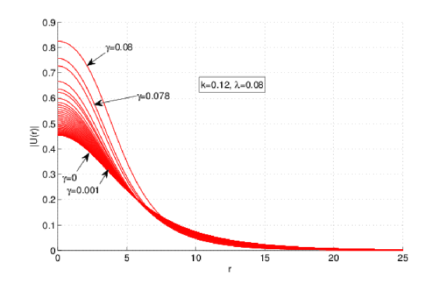
Figure 1: (Color on line) A set of radial profiles of the 2D $\mathcal{PT}$-symmetric solitons, found in the numerical form at a fixed propagation constant, $k=0.12$, and coupling constant $\lambda=0.08$, for various values of the gain-loss parameter, $\gamma=0,0.001...,0.08$.

Figure 1 shows that the soliton’s amplitude, $U(r=0)$, increases with the growth of $\gamma$, in accordance to the fact that combination (29) increases with $\gamma$. The dependence of the amplitude on $\gamma$ and $k$, for the same coupling constant as in Fig. 1, $\lambda=0.08$, is presented in Fig. 2 [strictly speaking, the amplitude also depends on the single combination $k_{\mathrm{eff}}$, see Eq. (29), but it makes sense to display the dependence of the amplitude on $\gamma$ for various constant values of $k$).

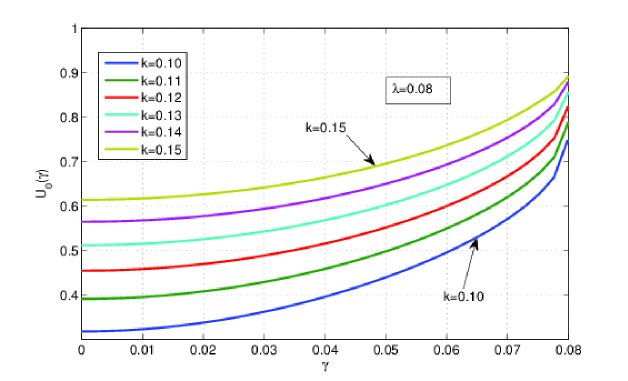
Figure 2: (Color on line). The soliton’s amplitude, $U(r=0)\equiv U_{0}(\gamma)$, as a function of $\gamma$ for a fixed coupling constant, $\lambda=0.08$, and different propagation constants $k$.

III.2 Stability limits for the solitons

As mentioned above, Eq. (3) essentially reduces the shape of the 2D fundamental $\mathcal{PT}$-symmetric solitons to that which was found, in another context, in Ref. Sweden . A new issue in the context of the $\mathcal{PT}$ symmetry is the stability of the solitons, beneath boundary (28) [recall that the solitons are completely stable above it, with $\lambda_{\max}^{\mathrm{(2D)}}$ found in the numerical form as indicated in Ref. (21), or approximated analytically as per Eq. (26)].

We studied the stability of the 2D $\mathcal{PT}$-symmetric solitons through the calculation of eigenvalues, $\sigma$, for modes of small perturbations governed by the linearization of Eqs. (1) and (2) around the stationary solitons, using methods elaborated in Ref. Yang:2010a . The main results are summarized in Figs. 3 and 4, which show the dependence of the largest instability growth rate, $S=\max\left\{\mathrm{Re}(\sigma)\right\}>0$, on $\gamma$ (in fact, the unstable eigenvalues are complex ones), for two different values of the coupling constant, $\lambda=0.08$ and $0.06$, and a set of fixed values of the propagation constant from the ranges of $0.12\leq k\leq 0.15$ and $0.09\leq k\leq 0.14$, respectively.

The ground-state $\mathcal{PT}$-symmetric solitons are stable in the region where $S(\gamma)=0$, i.e., at $\gamma<\gamma_{\mathrm{C}}\approx 0.008$ and $\gamma<\gamma_{\mathrm{C}}\approx 0.006$ in the former and latter cases, respectively. These critical values are essentially smaller (roughly, by a factor of $10$) than the respective maximum possible values of the gain-loss coefficient, $\gamma_{\max}=\lambda$, see Eq. (7), because the 2D solitons were taken at points which are close to the symmetry-breaking instability threshold in the usual coupler model, with $\gamma=0$, cf. Ref. Dror:2011a . A typical example of a stable soliton is displayed in inset (a) to Fig. Fig. 3.

The critical value, $\gamma_{\mathrm{C}}$, depends on $k$, as shown in detail in inset (b) to Fig. 3, and in the inset to Fig. 4. Naturally, $\gamma_{\mathrm{C}}$ increases with the decrease of $k$, as smaller $k$ correspond to a smaller energy of the soliton, pushing it farther from the symmetry-breaking threshold. However, the computation for $k$ essentially smaller than those presented in Figs. 3 and 4 is difficult, as the soliton becomes too broad, and cannot fit to the domain employed for the numerical solution.

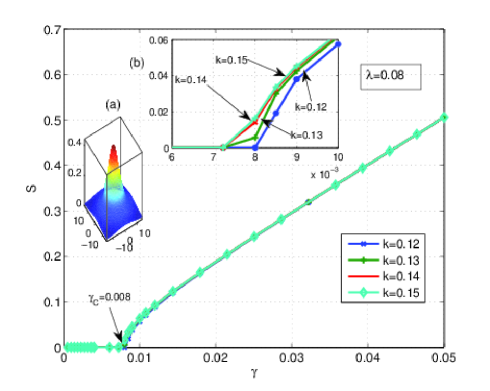
Figure 3: (Color online) The largest instability growth rate for eigenmodes of small perturbations around the $\mathcal{PT}$-symmetric 2D solitons, $S(\gamma)=\max\left\{\mathrm{Re}(\sigma)\right\}\geq 0$ [$\sigma$ is a complex eigenvalue of the linear-stability spectrum], for the fixed coupling constant, $\lambda=0.08$, and several values of the propagation constant, $k=0.12$, $0.13$, $0.14$, $0.15$, versus the gain-loss coefficient, $\gamma$. Inset (a) shows the profile of a typical stable soliton, found at $k=0.12$ and $\gamma=0.002$. Inset (b) is a blowup of a vicinity of the destabilization transition. For all these values of $k$, the destabilization occurs around the critical value, $\gamma_{\mathrm{C}}\approx 0.008$. The solitons are stable in the region of $S(\gamma)=0$.

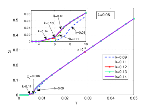
Figure 4: (Color online) The same as in Fig. 3, but for $\lambda=0.06$, and propagation constants $k=0.09$, $k=0.11$, $0.12$, $0.13$, $0.14$. The inset zooms in on a vicinity of the destabilization transition.

The predictions of the stability and instability, produced by the computation of the eigenvalues for perturbation modes, were verified by direct simulations of Eqs. (11)-(12), which were carried out by means of the split-step method CppRecipes2002 . The numerical algorithm was set in the $\left(x,y\right)$ domain of size $30\times 30$ [in the same notation in which Eqs. (11) and (12) are written] with periodic boundary conditions. The domain was covered by a discretization mesh of $256\times 256$ points. Because the instability of the soliton, if any, is caused by the breakup of the symmetry between the $\Psi$ and $\Phi$ components, which are subject to the action of the gain and loss, respectively [see Eqs. (11) and (12)], the initial perturbation in the simulations was introduced by multiplying the two components, severally, by the following factors:

$$\Psi_{0}\left(x,y\right)\rightarrow 1.03\times\Psi_{0}\left(x,y\right),~{}\Phi_{0}\left(x,y\right)\rightarrow~{}0.97\times\Phi_{0}\left(x,y\right).$$ (30)

A typical example of the perturbed evolution of a stable soliton is displayed in Fig. 5 [it is the same soliton whose stationary shape is displayed in inset (a) of Fig. 3]. The simulations demonstrate the stability of the soliton in the course of the evolution over the propagation distance which corresponds, roughly, to $20$ diffraction lengths of the soliton (in fact, the simulations confirm the stability over much longer distances).

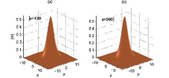
Figure 5: (Color online) An example of the long-distance evolution of a stable $\mathcal{PT}$-symmetric soliton, produced by direct simulations of Eqs. (11) and (12) with perturbed initial conditions [see Eq. (30)], starting from $z=0$. Panels (a) and (b) show the shape of the $\Psi$ component at $z=120$ and $z=500$, respectively. The evolution of the $\Phi$ component is similar. The parameters are $k=0.12$, $\lambda=0.08$, $\gamma=0.002$.

An example of the unstable evolution, observed at $\gamma=0.078>\gamma_{\mathrm{C}}$, is displayed in Fig. 6. The initial perturbation was again introduced as per Eq. (30); without the perturbation, the soliton may seem stable in the course of a long simulation, as the instability is quite weak. As seen in in Fig. 6, the transmission over distance $z\simeq 150$, which is estimated as $\sim 6$ diffraction lengths, leads to destruction of the soliton. In fact, this propagation distance is long, which once again stresses that we are here dealing with weak instability. Moreover, it is relevant to note that the value of $\gamma=0.078$, selected for this simulation, is very close to $\gamma_{\max}=\lambda=0.08,$ see Eq. (7). For smaller values of $\gamma$, Fig. 3 suggests that the propagation distance necessary for the development of the instability, $z_{\mathrm{instab}}\sim S^{-1}$, may be an order of magnitude larger than in Fig. 6. This conclusion suggests that, in terms of physical applications (such as collisions between solitons, see  below), unstable solitons may actually be robust objects.

Getting back to the analysis of the instability development, Fig. 6 demonstrates, that, as may be expected, the $\Phi$ component of the unstable soliton decays into a vanishingly small pattern under the action of the linear loss. On the other hand, the pump of energy by the gain into the $\Psi$ component does not cause an indefinite growth of its amplitude, but rather makes this component progressively “fatter” (broader). The latter result is easily explained by the character of the 2D fundamental-soliton solutions of the single NLS equation with the CQ nonlinearity: in the limit of large energy, the amplitude of the soliton is bounded by the largest value given by Eq. (20), $U_{\max}=\sqrt{3}/2\approx\allowbreak 0.87$, which is consistent with Figs. 6(c,e), while the effective radius of the “fat” soliton, $R$, is related to its total energy as $E\approx\pi R^{2}U_{\max}^{2}=\left(3/4\right)\pi R^{2}$. In the combination with the energy-balance equation (10), this argument predicts that the radius of the unstable soliton eventually grows exponentially, $R(z)\approx R_{0}\exp\left(\gamma z\right)$.

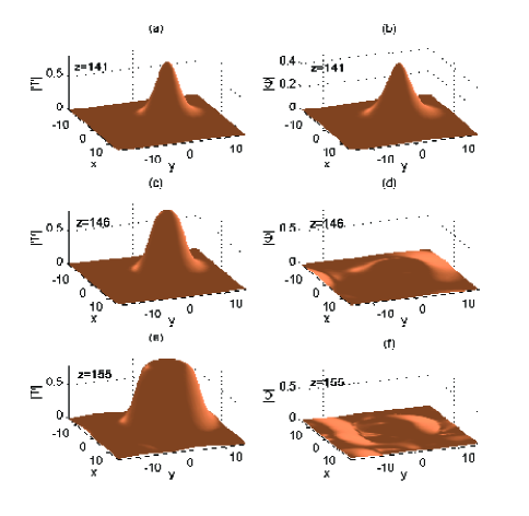
Figure 6: (Color on line) The evolution of $\Psi$ and $\Phi$ components of the unstable soliton (initiated at $z=0$) in the case of $k=0.12$, $\lambda=0.08$ and $\gamma=0.078>\gamma_{\mathrm{C}}$. The panels display the shapes of the two components at indicated values of the propagation distance.

III.3 Collisions between solitons

Because the underlying equations, (11) and (12), maintain the Galilean invariance, in spite of the presence of the gain and loss terms in them, the application of the kick to the soliton,

$$\left\{\Psi,\Phi\right\}\rightarrow\exp\left(i\mathbf{qr}\right)\left\{\Psi,\Phi\right\},$$ (31)

will set it in motion with velocity $\mathbf{V}=2\mathbf{q}$ [in fact, it is a tilt in the $\left(x,y,z\right)$ space]. Then, comparison with the work previously done for fundamental solitons in the single-core CQ model Sweden ; interaction suggests to consider collisions between moving (tilted) 2D solitons in the present  model. A straightforward consideration of physical parameters relevant for the optical waveguides demonstrates that $q\sim 1$ in the present notation corresponds to the tilt of the propagation direction $\sim 0.1^{\mathrm{o}}$.

Strictly speaking, the collisions should be considered only between fully stable solitons. However, it was shown above that those solitons which are unstable may be subject to a very weak instability. The propagation distance needed for simulating collisions between solitons is actually much smaller than the above-mentioned instability distance. Therefore, the consideration of collisions between weakly unstable solitons is meaningful too.

To simulate the collisions, two well-separated replicas of a stationary soliton, with phase shift $\phi$ between them, were created and kicked in opposite directions as per Eq. (31), i.e., with factors $\exp\left(\pm i\mathbf{qr}\right)$, so as to initiate the head-on collision between them. An example of the simulated collision between two identical in-phase ($\phi=0$) solitons with the same parameters as in Fig. 6 is displayed in Fig. 7, for kicks $q=0.4$. It is seen that the collision is inelastic but not destructive. It gives rise to a spontaneous symmetry breaking between the solitons, making one of them taller than the other. The effect of the symmetry breaking between colliding solitons is known in other models, see, e.g., Ref. Javid . After the collision, the two asymmetric solitons separate. The $\mathcal{PT}$ symmetry is kept intact in the course of the collision (therefore, only the $\Phi$ component is displayed in Fig. 6), in spite of the fact that the colliding solitons are classified, strictly speaking, as unstable ones. The robustness of the setting against breaking of the $\mathcal{PT}$ symmetry is explained by the fact that the collision happens over propagation distance $z\simeq 15$, which is ten times smaller than the distance necessary for the manifestation of the instability, cf. Fig. 6.

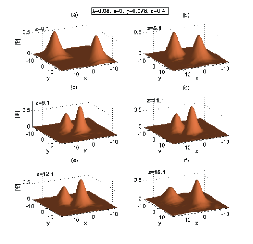
Figure 7: (Color on line) Collision between two identical solitons with zero phase shift, kicked as per Eq. (31) in the opposite directions by $q=0.4$. The panels display the shapes of the $\Psi$-components at indicated values of the propagation distance. The evolution of the $\Phi$ component is the same, as the collision does not break the $\mathcal{PT}$ symmetry. The parameters are $k=0.12$, $\lambda=0.08$, $\gamma=0,078$.

The collision induced by a larger kick, $q=1$, gives rise to a still stronger effect of the spontaneously symmetry breaking between the two solitons, as shown in Fig. 8: one of the solitons temporarily splits into two peaks of different heights, and later recombines back into a single one. Nevertheless, in this case too, the collision does not break the $\mathcal{PT}$ symmetry, which demonstrates the dynamical robustness of this property.

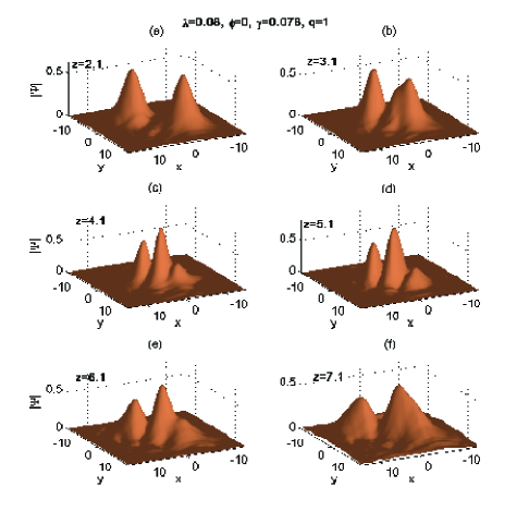
Figure 8: (Color on line) The same as in Fig. 7, except that the initial kick is larger, $q=1$.

We have also performed systematic simulations of collisions between fully stable solitons, with $\gamma<\gamma_{\mathrm{C}}$, and also between formally unstable or fully stable ones with the phase shift of $\phi=\pi$. The results (not shown here in detail) demonstrate that truly stable solitons collide in exactly the same fashion as their formally unstable counterparts, i.e., like in Fig. 7 or Fig. 8 at smaller and larger values of the kick, respectively. The introduction of the phase shift $\phi=\pi$ does not change the results conspicuously either (one may expect that the phase shift will be important in the case of very small collision velocities Javid ).

IV Conclusion

We have considered 1D solitons (in a brief form), and their 2D counterparts (systematically) in the model of the $\mathcal{PT}$-symmetric coupler, which is characterized by the mutually balanced linear gain and loss applied to its cores, in the combination with the CQ (cubic-quintic) intrinsic nonlinearity acting in both cores. The self-defocusing quintic term is necessary to protect the solitons against the usual 2D collapse. The model can be realized in terms of the spatiotemporal transmission in dual-core optical waveguides. The $\mathcal{PT}$-symmetric solitons lose their stability with the increase of the energy, and restore the stability at still larger energies. The boundary value of the linear-coupling strength, above which the symmetric solitons are completely stable, was found by means of an analytical approximation (using the exact solution for the CW version of the system), which is rather close to its numerically found counterparts for the 1D and 2D solitons. Stability limits of the 2D solitons and evolution of the unstable ones were investigated in the numerical form, by means of the computation of stability eigenvalues and direct simulations. Although large parts of the soliton families are unstable, the instability is quite weak, making it possible to use formally unstable solitons in physical applications. Head-on collisions between solitons were studied in a systematic form too, demonstrating that the collisions break the symmetry between identical solitons, but do not break the $\mathcal{PT}$ symmetry.

It may be interesting to extend the 2D analysis of the same model to vortex solitons. Starting from pioneering works Manolo and Bob , the stability of 2D vortex solitons in the single-core system with the CQ nonlinearity was a subject of many studies vort-CQ . For the dual-core CQ system, the analysis of the vortex-soliton stability was reported in Ref. Dror:2011a . The $\mathcal{PT}$-symmetric generalization of such settings may be the next natural step.

References

- (1) C. M. Bender, Rep. Prog. Phys. 70, 947 (2007).
- (2) See special issues: H. Geyer, D. Heiss, and M. Znojil, Eds., J. Phys. A: Math. Gen. 39, Special Issue Dedicated to the Physics of Non-Hermitian Operators (PHHQP IV) (University of Stellenbosch, South Africa, 2005) (2006); A. Fring, H. Jones, and M. Znojil, Eds., J. Math. Phys. A: Math Theor. 41, Papers Dedicated to the Subject of the 6th International Workshop on Pseudo-Hermitian Hamiltonians in Quantum Physics (PHHQPVI) (City University London, UK, 2007) (2008); C. Bender, A. Fring, U. Günther, and H. Jones, Eds., Special Issue: Quantum Physics with non-Hermitian Operators, J. Math. Phys. A: Math Theor. 41, No. 44 (2012).
- (3) A. Ruschhaupt, F. Delgado, and J. G. Muga, J. Phys. A: Math. Gen. 38, L171 (2005); R. El-Ganainy, K. G. Makris, D. N. Christodoulides, and Z. H. Musslimani, Opt. Lett. 32, 2632 (2007); M. V. Berry, J. Phys. A: Math. Theor. 41, 244007 (2008).
- (4) A. Guo, G. J. Salamo, D. Duchesne, R. Morandotti, M. Volatier-Ravat, V. Aimez, G. A. Siviloglou, and D. N. Christodoulides, Phys. Rev. Lett. 103, 093902 (2009); C. E. Rüter, K. G. Makris, R. El-Ganainy, D. N. Christodoulides, M. Segev, and D. Kip, Nature Phys. 6, 192 (2010); A. Regensburger, C. Bersch, M.-A. Miri, G. Onishchukov, D. N. Christodoulides, and U. Peschel, Nature 488, 167 (2012).
- (5) K. G. Makris, R. El-Ganainy, D. N. Christodoulides, and Z. H. Musslimani, Phys. Rev. Lett. 100, 103904 (2008); S. Longhi, Phys. Rev. A 81, 022102 (2010).
- (6) K. G. Makris, R. El-Ganainy, D. N. Christodoulides, and Z. H. Musslimani, Int. J. Theor. Phys. 50, 1019 (2011).
- (7) Z. H. Musslimani, K. G. Makris, R. El-Ganainy, and D. N. Christodoulides, Phys. Rev. Lett. 100, 030402 (2008); Z. Lin, H. Ramezani, T. Eichelkraut, T. Kottos, H. Cao, and D. N. Christodoulides, Phys. Rev. Lett. 106, 213901 (2011); X. Zhu, H. Wang, L.-X. Zheng, H. Li, and Y.-J. He, Opt. Lett. 36, 2680 (2011); C. Li, H. Liu, and L. Dong, Opt. Exp. 20, 16823 (2012); C. M. Huang, C. Y. Li, and L. W. Dong, ibid. 21, 3917 (2013).
- (8) S. Nixon, L. Ge, and J. Yang, Phys. Rev. A 85, 023822 (2012).
- (9) H. G. Li, Z. W. Shi, X. J. Jiang, and X. Zhu, Opt. Lett. 36, 3290 (2011); V. Achilleos, P. G. Kevrekidis, D. J. Frantzeskakis, and R. Carretero-González, Phys. Rev. A 86, 013808 (2012).
- (10) F. C. Moreira, F. K. Abdullaev, V. V. Konotop, and A. V. Yulin, Phys. Rev. A 86, 053815 (2012); F. C. Moreira, V. V. Konotop, and B. A. Malomed, ibid. 87, 013832 (2013).
- (11) S. V. Dmitriev, A. A. Sukhorukov, and Y. S. Kivshar, Opt. Lett. 35, 2976 (2010); S. V. Suchkov, B. A. Malomed, S. V. Dmitriev, and Y. S. Kivshar, Phys. Rev. E 84, 046609 (2011); S. V. Suchkov, A. A. Sukhorukov, S. V. Dmitriev, and Y. S. Kivshar, EPL 100, 54003 (2012); D. A. Zezyulin and V. V. Konotop, Phys. Rev. Lett. 108, 213906 (2012).
- (12) D. Leykam, V. V. Konotop, and A. S. Desyatnikov, Opt. Lett. 38, 371 (2013); I. V. Barashenkov, L. Baker, and N. V. Alexeeva, Phys. Rev. A 87, 033819 (2013).
- (13) K. Li and P. G. Kevrekidis, Phys. Rev. E 83, 066608 (2011); V. V. Konotop, D. E. Pelinovsky, and D. A. Zezyulin, EPL 100, 56006 (2012); J. D’Ambroise, P. G. Kevrekidis, and S. Lepri, J. Phys. A: Math. Theor. 45, 444012 (2012); K. Li, P. G. Kevrekidis, B. A. Malomed, and U. Günther, ibid. 45, 444021 (2012); M. Kreibich, J. Main, H. Cartarius, and G. Wunner, Phys. Rev. A 87, 051601(R) (2013).
- (14) B. A. Malomed, Physica D 29, 155 (1987); S. Fauve, O. Thual, Phys. Rev. Lett. 64, 282 (1990); W. van Saarloos and P. C. Hohenberg, Phys. Rev. Lett. 64, 749 (1990); V. Hakim, P. Jakobsen, and Y. Pomeau, Europhys. Lett. 11, 19 (1990); B. A. Malomed and A. A. Nepomnyashchy, Phys. Rev. A 42, 6009 (1990); P. Marcq, H. Chaté, and R. Conte, Physica D 73, 305 (1994); T. Kapitula and B. Sandstede, J. Opt. Soc. Am. B 15, 2757 (1998); A. Komarov, H. Leblond, and F. Sanchez, Phys. Rev. E 72, 025604 (2005).
- (15) J. N. Kutz, SIAM Rev. 48, 629 (2006).
- (16) F. Kh. Abdullaev, Y. V. Kartashov, V. V. Konotop, and D. A. Zezyulin, Phys. Rev. A 83, 041805(R) (2011); D. A. Zezyulin, Y. V. Kartashov, V. V. Konotop, Europhys. Lett. 96, 64003 (2011); A. E. Miroshnichenko, B. A. Malomed, and Y. S. Kivshar, Phys. Rev. A 84, 012123 (2011).
- (17) Y. He, X. Zhu, D. Mihalache, J. Liu, and Z. Chen, Phys. Rev. A 85, 013831 (2012); Opt. Commun. 285, 3320 (2012).
- (18) R. Driben and B. A. Malomed, Opt. Lett. 36, 4323 (2011).
- (19) N. V. Alexeeva, I. V. Barashenkov, A. A. Sukhorukov, and Y. S. Kivshar, Phys. Rev. A 85, 063837 (2012).
- (20) R. Driben and B. A. Malomed, Europhys. Lett. 94, 37011 (2011); I. V. Barashenkov, S. V. Suchkov, A. A. Sukhorukov, S. V. Dmitriev, and Y. S. Kivshar, Phys. Rev. A 86, 053809 (2012).
- (21) F. K. Abdullaev, V. V. Konotop, M. Ögren, and M. P. Sørensen, Opt. Lett. 36, 4566 (2011); Yu. V. Bludov, V. V. Konotop, and B. A. Malomed, Phys. Rev. A 87, 013816 (2013); Yu. V. Bludov, R. Driben, V. V. Konotop, and B. A. Malomed, J. Opt. 15, 064010 (2013).
- (22) N. Dror and B. A. Malomed, Physica D 240, 526 (2011).
- (23) E. M. Wright, G. I. Stegeman, and S. Wabnitz, Phys. Rev. A 40, 4455 (1989); M. Romagnoli, S. Trillo, and S. Wabnitz, Opt. and Quant. Elect. 24, S1237 (1992).
- (24) C. Paré and M. Fłorjańczyk, Phys. Rev. A 41, 6287 (1990); A. I. Maimistov, Kvantovaya Elektron. (Moscow) 18, 758 (1991) [English translation:, Sov. J. Quantum Electr., 21, 687 (1991)]; N. Akhmediev and A. Ankiewicz, Phys. Rev. Lett. 70, 2395 (1993); J. M. Soto-Crespo and N. Akhmediev, Phys. Rev. E 48, 4710 (1993); P. L. Chu, B. A. Malomed, and G. D. Peng, J. Opt. Soc. Am. B 10, 1379 (1993); B. A. Malomed, I. Skinner, P. L. Chu, and G. D. Peng, Phys. Rev. E 53, 4084 (1996); W. C. K. Mak, B. A. Malomed, and P. L. Chu, J. Opt. Soc. Am. B 15, 1685 (1998).
- (25) W. C. K. Mak, B. A. Malomed and P. L. Chu, Phys. Rev. E 55, 6134 (1997); ibid. 57, 1092 (1998).
- (26) Spontaneous Symmetry Breaking, Self-Trapping, and Josephson Oscillations, B. A. Malomed, editor (Springer-Verlag: Berlin and Heidelberg, 2013).
- (27) J. Yang, Stud. Appl. Math., in press.
- (28) L. Bergé, Phys. Rep. 303, 259 (1998); E. A. Kuznetsov and F. Dias, ibid. 507, 43 (2011).
- (29) G. S. Agarwal and S. Dutta Gupta, Phys. Rev. A 38, 5678 (1988); F. Smektala, C. Quemard, V. Couderc, A. Barthélémy, J. Non-Cryst. Solids 274, 232 (2000); C. Zhan, D. Zhang, D. Zhu, D. Wang, Y. Li, D. Li, Z. Lu, L. Zhao, Y. Nie, J. Opt. Soc. Am. B 19, 369 (2002); G. Boudebs, S. Cherukulappurath, H. Leblond, J. Troles, F. Smektala, F. Sanchez, Opt. Commun. 219, 427 (2003); F. Sanchez, G. Boudebs, S. Cherukulappurath, H. Leblond, J. Troles, F. Smektala, J. Nonlin. Opt. Phys. & Mat. 13, 7 (2004); K. Ogusu, J. Yamasaki, S. Maeda, M. Kitao, M. Minakata, Opt. Lett. 29, 265 (2004); E. L. Falcão-Filho, C. B. de Araújo, and J. J. Rodrigues, Jr., J. Opt. Soc. Am. B 24, 2948 (2007).
- (30) B. A. Malomed, D. Mihalache, F. Wise, and L. Torner, J. Opt. B: Quant. Semicl. Opt. 7, R53 (2005).
- (31) L. Albuch and B. A. Malomed, Mathematics and Computers in Simulation 74, 312 (2007).
- (32) Z. Birnbaum and B. A. Malomed, Physica D 237, 3252 (2008).
- (33) L. Gubeskys and B. A. Malomed, J. Opt. Soc. Am. B 30, 1843 (2013).
- (34) Kh. I. Pushkarov, D. I. Pushkarov, and I. V. Tomov, Opt. Quant. Electr. 11, 471 (1979); S. Cowan, R. H. Enns, S. S. Rangnekar, S. S. Sanghera, Can. J. Phys. 64, 311 (1986).
- (35) M. L. Quiroga-Teixeiro, A. Berntson, and H. Michinel, J. Opt. Soc. Am. B 16, 1697 (1999).
- (36) D. Novoa, H. Michinel, and D. Tommasini, Phys. Rev. Lett. 103, 023903 (2009).
- (37) J. Yang, Nonlinear Waves in Integrable and Non-integrable Systems (SIAM: Philadelphia, 2010).
- (38) W. H. Press, S. A. Teukovsky, W. T. Vetterling, and B. P. Flannery, Numerical recipes in C++ , Chap. 17 (Cambridge University Press: Cambridge, 2002).
- (39) S. Konar, S. Jana, and M. Mishra, Opt. Commun. 255, 114 (2005).
- (40) J. Atai and B. A. Malomed, Phys. Rev. E 64, 066617 (2001).
- (41) M. Quiroga-Teixeiro and H. Michinel, J. Opt. Soc. Am. B 14, 2004 1997).
- (42) R. L. Pego and H. A. Warchall, J. Nonlin. Sci. 12, 347 (2002).
- (43) I. Towers, A. V. Buryak, R. A. Sammut, B. A. Malomed, L. C. Crasovan, and D. Mihalache, Phys. Lett. A 288, 292 (2001); B. A. Malomed, L.-C. Crasovan, and D. Mihalache, Physica D 161, 187 (2002); T. A. Davydova and A. I. Yakimenko, J. Opt. A: Pure Appl. Opt. 6, S197 (2004); H. Michinel, J. R. Salgueiro, and M. J. Paz-Alonso, Phys. Rev. E 70, 066605 (2004); M. J. Paz-Alonso and H. Michinel, Phys. Rev. Lett. 94, 093901 (2005); L. Dong, J. Wang, H. Wang, and G. Yin, Phys. Rev. A 79, 013807 (2009).