A New Algorithm for Distributed Nonparametric Sequential Detection

Abstract

We consider nonparametric sequential hypothesis testing problem when the distribution under the null hypothesis is fully known but the alternate hypothesis corresponds to some other unknown distribution with some loose constraints. We propose a simple algorithm to address the problem. These problems are primarily motivated from wireless sensor networks and spectrum sensing in Cognitive Radios. A decentralized version utilizing spatial diversity is also proposed. Its performance is analysed and asymptotic properties are proved. The simulated and analysed performance of the algorithm is compared with an earlier algorithm addressing the same problem with similar assumptions. We also modify the algorithm for optimising performance when information about the prior probabilities of occurrence of the two hypotheses are known.

I Introduction

Presently there is a scarcity of spectrum due to the proliferation of wireless services. Cognitive Radios (CRs) are proposed as a solution to this problem. It has been observed that much of the licensed spectrum remains unutilised for most of the time. CRs are designed to exploit these gaps and use them for communication, without causing interference to the primary users. This is achieved through spectrum sensing by the CRs, to gain knowledge about spectrum usage by the primary users.

Distributed detection has been a highly-studied topic recently, due to its relevance to various physical scenarios such as sensor networks ([vvv2007sensor], [varshney97sensors]), cooperative spectrum sensing in cognitive radios ([Akyildiz06nextgenerationdynamic]), and so on. This approach reduces error probabilities and detection delays through the use of spatial multiplexing.

Distributed detection problems can be looked upon either is centralised or decentralised framework. In a centralised algorithm, the information collected by the local nodes are transmitted directly to the fusion centre. In a decentralised algorithm, the local nodes transmit certain quantised values of the information. This has the advantage of requiring less power and bandwidth, but is suboptimal since the fusion centre has to take a decision based on less information.

The distributed detection problem can also be classified as fixed sample or sequential. In a fixed sample framework, the decision has to be made based on a fixed number of samples, and the likelihood ratio test turns out to be optimal. In a sequential framework, samples are taken until some conditions are fulfilled, and once the process of taking samples has stopped, a decision is arrived at.

[dualsprt] and [uscslrt] have studied the distributed decentralised detection problem in a sequential framework, with a noisy reporting MAC. The algorithm in [dualsprt] requires complete knowledge of the probability distributions involved, and is thus parametric in nature. The approach in [uscslrt] is non-paramteric in the sense that it assumes very little knowledge of one of the distributions. In this paper, we have presented a simpler algorithm to address the same problem as studied in [uscslrt]. Our algorithm has the added advantage of better performance in most cases, as borne out by simulations and analysis.

II System Model

There are L nodes and one fusion centre. The setup is i.i.d. We have have to decide between the hypotheses:

$H_{0}$: the probability distribution is $P_{0}$, and
$H_{1}$: the probability distribution is $P_{1}$

$P_{0}$ is known, but nothing is known about $P_{1}$, except that it is stationary, $D(P_{1}||P_{0})\geq\lambda$, where $\lambda$ is known, and$H(P_{1})\geq H(P_{0})$

At the local node $l$, if $X_{k,l}$ be the signal received at time k, then the test statistic at the $k^{th}$ instant is given by

$\widetilde{W}_{k,l}^{\mbox{new}}$ $=$ $-\log[P_{0}(X_{1,l}^{k})]-k.H(P_{0})-\frac{k\lambda}{2}$

or by

$\widetilde{W}_{k,l}^{\mbox{new}}$ $=$ $-\log[P_{0}(X_{1,l}^{k})]-k.h(P_{0})-\frac{k\lambda}{2}$,
depending on whether the distribution $P_{0}$ is discrete or continuous.

Symbol	Definition
L	Number of nodes
$X_{k,l}$	Observation at node $l$ at time $k$
$Y_{k,l}$	Transmitted value from node $l$ to FC at time $k$
$Y_{k}$	FC observation at time k
$Z_{k}$	Fusion Centre MAC noise at time $k$
$f_{i,l}$	pdf of $X_{k,l}$ under $H_{i}$
$\widetilde{W}_{k,l}^{\mbox{new}}$	test statistic at node $l$ at time $k$
$g_{\mu}$	pdf of $Z_{k}+\mu$
$F_{k}$	test statistic at fusion centre at time $k$
$\xi_{k}$	LLR process at fusion centre $=\log\frac{g_{\mu_{1}}(Y_{k})}{g_{-\mu_{0}}(Y_{k})}$
$\xi_{k}^{*}$	LLR process at fusion centre when all local nodes
	transmit wrong decisions
$\theta_{i}$	$E_{i}(\xi_{k}^{*})$
$\mathcal{A}^{i}$	$\{\omega\in\Omega:\mbox{all local nodes transmit correct decisions }(b_{i})\mbox{ under }H_{i}\}$
$\Delta(\mathcal{A}^{i})$	Drift of fusion centre LLR under $\mathcal{A}^{i}$, i.e. $E_{i}[\xi_{k}|\mathcal{A}^{i}]$
$-\log(\alpha_{l})$, $\log(\beta_{l})$	Higher and lower thresholds, respectively, at local node $l$
$-\log(\alpha)$, $\log(\beta)$	Higher and lower thresholds, respectively, at fusion centre
$\mu_{1}$, $\mu_{0}$	Values for adjusting the fusion centre LLR
$b_{1}$, $b_{0}$	Values transmitted to the fusion centre from local nodes
$N_{l}$	$\inf\{k:\widetilde{W}_{k,l}^{\mbox{new}}\notin(\log(\beta_{l}),-\log(\alpha_{l}))\}$
$N_{l}^{1}$, $N_{l}^{0}$	$\inf\{k:\widetilde{W}_{k,l}^{\mbox{new}}\geq-\log(\alpha_{l})\}$, $\inf\{k:\widetilde{W}_{k,l}^{\mbox{new}}\leq\log(\beta_{l})\}$
$N$	$\inf\{k:F_{k}\notin(\log(\beta),-\log(\alpha))\}$
$N^{1}$, $N^{0}$	$\inf\{k:F_{k}\geq-\log(\alpha)\}$, $\inf\{k:F_{k}\leq\log(\beta)\}$
$V_{k,l}$	$\widetilde{W}_{k+1,l}^{\mbox{new}}-\widetilde{W}_{k,l}^{\mbox{new}}$
$\delta_{i,l}$, $\rho_{i,l}^{2}$	Mean and variance of $V_{k,l}$ under $H_{i}$
$\delta^{j}_{i,FC}$	mean drift of the fusion centre LLR when $j$ local nodes transmit,
	under $H_{i}$
$t_{j}$	time point when $\delta^{j-1}_{i,FC}$ changes into $\delta^{j}_{i,FC}$
$\tilde{F}_{j}$	$E[F_{t_{j}-1}]$
$D^{0}_{tot}$	$\frac{L\lambda}{2}$

$D^{1}_{tot}$	$\displaystyle\sum_{l=1}^{L}[D(f_{1,l}||f_{0,l})+H(f_{1,l})-H(f_{0,l})-\frac{\lambda}{2}]$
$r_{l}$	$\frac{1}{L}$
$\rho_{l}$	$\frac{D(f_{1,l}||f_{0,l})+H(f_{1,l})-H(f_{0,l})-\frac{\lambda}{2}}{D^{1}_{tot}}$
$R_{i}$	$\displaystyle\min_{1\leq l\leq L}\{-\log\inf_{t\geq 0}E_{i}[\exp\{-t(-\log f_{0,l}(X_{k,l})-H(P_{0})-\frac{\lambda}{2})\}]\}$
$g_{i}$, $\hat{g_{i}}$	MGF of $|\xi_{k}^{*}|$, $\xi_{k}^{*}$
$\Lambda_{i}(\alpha)$, $\hat{\Lambda_{i}}(\alpha)$	$\displaystyle\sup_{\lambda}[a\lambda-\log g_{i}(\lambda)]$, $\displaystyle\sup_{\lambda}[a\lambda-\log\hat{g_{i}}(\lambda)]$
$\alpha_{i}^{+}$	$\mbox{ess}\sup|\xi_{k}^{*}|$
$\mathcal{R}_{c}(\delta)$	Bayes risk of test $\delta$ with cost of each observation $=c$
$l_{i}^{*}$	$\min\{j:\delta^{j}_{i,FC}>0\mbox{ and }\frac{\mbox{ corresponding threshold }-\tilde{F_{j}}}{\delta^{j}_{i,FC}}<E(t_{j+1})-E(t_{j})\}$
$N_{0}^{*}(\epsilon)$, $N_{1}^{*}(\epsilon)$	$\sup\{n\geq 1:|-\log P_{0}(x_{1}^{n})-nH(P_{0})|>n\epsilon\}$,
	$\sup\{n\geq 1:|-\log P_{0}(x_{1}^{n})-nH(P_{1})-nD(P_{1}||P_{0})|>n\epsilon\}$

TABLE I: Symbols and Letters

III Results for a Single Node

Let

$N_{1}\triangleq\inf\{n:\mbox{ }\widetilde{W}_{n}^{\mbox{new}}>-\log\alpha\}$

$N_{0}\triangleq\inf\{n:\mbox{ }\widetilde{W}_{n}^{\mbox{new}}<\log\beta\}$

$N\triangleq\mbox{ stopping time}=\min(N_{0},N_{1})$

$\mathbf{Lemma\mbox{ }3.1}$

$P(N<\infty)=1$ under $H_{0}$ and $H_{1}$.

$\mathbf{Proof}$: Under $H_{0}$,

$P_{0}(N<\infty)\geq P_{0}(N_{0}<\infty)$

$=P_{0}(\widetilde{W}_{n}^{\mbox{new}}<\log\beta\mbox{ for some postive integer }n)$

$=P_{0}(\frac{\widetilde{W}_{n}^{\mbox{new}}}{n}<\frac{\log\beta}{n}\mbox{ for some postive integer }n)$

$\geq P_{0}(\frac{\widetilde{W}_{m}^{\mbox{new}}}{m}<\frac{\log\beta}{m}\mbox{ for a particular postive integer }m)$
$\to 1$ as $m\to\infty$
(since under $H_{0}$, $\frac{\widetilde{W}_{m}^{\mbox{new}}}{m}\to-\frac{\lambda}{2}$ in probability)

The proof is similar under $H_{1}$


$\mathbf{Lemma\mbox{ }3.2}$
a)
$P_{FA}\triangleq P_{0}(\mbox{ decide }H_{1})=\mathcal{O}(\alpha^{s})$
where s is a solution of
$E_{0}[e^{-s(\frac{\lambda}{2}-\epsilon)}]=1$ where $0<\epsilon<\frac{\lambda}{2}$ and $s>0$

b)
$P_{MD}\triangleq P_{1}(\mbox{ decide }H_{0})=\mathcal{O}(\beta^{s^{*}})$
where $s^{*}$ is a solution of
$E_{1}[e^{-s^{*}(D(P_{1}||P_{0})+H(P_{1})-H(P_{0})-\frac{\lambda}{2}-\epsilon)}]=1$,
$0<\epsilon<D(P_{1}||P_{0})+H(P_{1})-H(P_{0})-\frac{\lambda}{2}$ and $s^{*}>0$

$\mathbf{Proof}$:
a)
$A_{n_{1}}(\epsilon)\triangleq\{x_{1}^{\infty}:|-\log P_{0}(x_{1}^{n})-nH(P_{0})|<n\epsilon\mbox{ }\forall\mbox{ }n\geq n_{1}\}$

For any $n_{1}>0$,
$P_{FA}=P_{0}(N_{1}<N_{0})$
$=P_{0}(N_{1}<N_{0};N_{1}\leq n_{1})$
$+P_{0}(N_{1}<N_{0};N_{1}>n_{1};A_{n_{1}}(\epsilon))$
$+P_{0}(N_{1}<N_{0};N_{1}>n_{1};A_{n_{1}}^{c}(\epsilon))$

By the strong law of large numbers, we can take $M_{1}>0$ such that $P_{0}(A_{n_{1}}^{c}(\epsilon))=0\mbox{ }\forall\mbox{ }n_{1}\geq M_{1}$. Let us choose such an $n_{1}$

$P_{0}(N_{0}<\infty)=1$

$\therefore P_{0}(N_{1}<N_{0};N_{1}>n_{1};A_{n_{1}}(\epsilon))$
$\leq P_{0}(N_{1}<\infty;N_{1}>n_{1};A_{n_{1}}(\epsilon))$

For $x_{1}^{\infty}\in A_{n_{1}}(\epsilon)$, for $n\geq n_{1}$,

$\widetilde{W}_{n}^{\mbox{new}}=-\log P_{0}(x_{1}^{n})-nH(P_{0})-\frac{n\lambda}{2}$

$\leq n\epsilon-\frac{n\epsilon}{2}$

By choosing $0<\epsilon<\frac{\lambda}{2}$, $\{\widetilde{W}_{n}^{\mbox{new}}\}$ is thus a random walk with an eventually negative drift.

Let $N_{0}^{1}$ be the stopping time of this random walk to cross $-\log\alpha\equiv|\log\alpha|$

Then, $P_{0}(n_{1}<N_{1}<\infty;A_{n_{1}}(\epsilon))\leq P_{0}(N_{0}^{1}<\infty)\leq e^{s^{\prime}|\log\alpha|}$,

where $s^{\prime}$ is the negative solution of $E_{0}[e^{s^{\prime}(\frac{\lambda}{2}-\epsilon)}]=1$. ([opac-b1086480], Chapter 4)

Finally, the first term in the expression for $P_{FA}$ can be written as $P_{0}(N_{1}<N_{0};N_{1}\leq n_{1})$
$\leq P_{0}(N_{1}\leq n_{1})$

$\leq\displaystyle\sum_{n=1}^{n_{1}}P_{0}(-\log P_{0}(X_{1}^{n})-nH(P_{0})-\frac{n\lambda}{2}\geq|\log\alpha|)$

$=\displaystyle\sum_{n=1}^{n_{1}}P_{0}(\log P_{0}(X_{1}^{n})+nH(P_{0})+\frac{n\lambda}{2}\leq-|\log\alpha|)$

$=0\mbox{ }\forall\mbox{ }\alpha<\alpha_{1}$, for some $\alpha_{1}>0$, since the L.H.S. is finite. Hence as $\alpha\to 0$, the first term is zero.

Hence, taking $s\triangleq-s^{\prime}$, $P_{FA}=\mathcal{O}(\alpha^{s})$.

By defining
$B_{n_{1}}(\epsilon)\triangleq\{x_{1}^{\infty}:|-\log P_{0}(x_{1}^{n})-nD(P_{1}||P_{0})-nH(P_{1})|<n\epsilon\mbox{ }\forall\mbox{ }n\geq n_{1}\}$, the proof for the next part follows similarly.

$\mathbf{Definitons}$
$N_{0}^{*}(\epsilon)\triangleq\sup\{n\geq 1:|-\log P_{0}(x_{1}^{n})-nH(P_{0})|>n\epsilon\}$

$N_{1}^{*}(\epsilon)\triangleq\sup\{n\geq 1:|-\log P_{0}(x_{1}^{n})-nH(P_{1})-nD(P_{1}||P_{0})|>n\epsilon\}$

$\mathbf{Lemma\mbox{ }3.3}$
a) Under $H_{0}$,
$\displaystyle\lim_{\alpha,\beta\to 0}\frac{N}{|\log\beta|}=\frac{2}{\lambda}$ a.s.

If in addition,$E_{0}(N_{0}^{*}(\epsilon)^{p})<\infty$ and $E_{0}[(\log P_{0}(X))^{p+1}]<\infty$
for all $\epsilon>0$ and for some $p\geq 1$, then

$\displaystyle\lim_{\alpha,\beta\to 0}\frac{E_{0}[N^{q}]}{|\log\beta|^{q}}=\displaystyle\lim_{\alpha,\beta\to 0}\frac{E_{0}[N_{0}^{q}]}{|\log\beta|^{q}}=(\frac{2}{\lambda})^{q}$

for all $0<q\leq p$.

b) Under $H_{1}$,
$\displaystyle\lim_{\alpha,\beta\to 0}\frac{N}{|\log\beta|}=\frac{1}{D(P_{1}||P_{0})+H(P_{1})-H(P_{0})-\frac{\lambda}{2}}$ a.s.

If in addition,$E_{1}(N_{1}^{*}(\epsilon)^{p})<\infty$ and $E_{1}[(\log P_{0}(X))^{p+1}]<\infty$
for all $\epsilon>0$ and for some $p\geq 1$, then

$\displaystyle\lim_{\alpha,\beta\to 0}\frac{E_{1}[N^{q}]}{|\log\beta|^{q}}$

$=\displaystyle\lim_{\alpha,\beta\to 0}\frac{E_{1}[N_{1}^{q}]}{|\log\beta|^{q}}$

$=(D(P_{1}||P_{0})+H(P_{1})-H(P_{0})-\frac{\lambda}{2})^{-q}$

for all $0<q\leq p$.
$\mathbf{Proof}$:
a)
$N=N_{0}\mathbbm{1}\{N_{0}\leq N_{1}\}$+$N_{1}\mathbbm{1}\{N_{0}>N_{1}\}$

Under $H_{0}$, $P_{FA}\to 0$ as $\alpha\to 0$ and hence,

$\displaystyle\lim_{\alpha,\beta\to 0}\frac{N}{|\log\beta|}=\displaystyle\lim_{\alpha,\beta\to 0}\frac{N_{0}\mathbbm{1}\{N_{0}\leq N_{1}\}}{|\log\beta|}$ a.s.

For $0<r<1$, we define

$A_{r}\triangleq\{\omega:\displaystyle\sup_{n\leq N_{0}^{*}(\epsilon)}\widetilde{W}_{n}^{\mbox{new}}\leq r|\log\beta|<|\log\alpha|\}$

For $n>N_{0}^{*}(\epsilon)$, $\widetilde{W}_{n}^{\mbox{new}}\leq n\epsilon-\frac{n\lambda}{2}$, i.e., $n\geq-\frac{\widetilde{W}_{n}^{\mbox{new}}}{\frac{\lambda}{2}-\epsilon}$

Hence, under $A_{r}$, if $N_{0}>N_{0}^{*}(\epsilon)$,

$N_{0}-N_{0}^{*}(\epsilon)\leq\frac{-\log\beta}{\frac{\lambda}{2}-\epsilon}-\frac{r\log\beta}{\frac{\lambda}{2}-\epsilon}=\frac{1+r}{\frac{\lambda}{2}-\epsilon}|\log\beta|$

Similarly under $A_{r}^{c}$,
$N_{0}-N_{0}^{*}(\epsilon)\leq\frac{-\log\beta}{\frac{\lambda}{2}-\epsilon}-\frac{\log\alpha}{\frac{\lambda}{2}-\epsilon}=\frac{|\log\alpha|+|\log\beta|}{\frac{\lambda}{2}-\epsilon}$

Hence, $N_{0}\mathbbm{1}\{N_{0}\leq N_{1}\}\leq N_{0}$
$\leq N_{0}^{*}(\epsilon)+\frac{1+r}{\frac{\lambda}{2}-\epsilon}|\log\beta|\mathbbm{1}\{A_{r}\}+\frac{|\log\alpha|+|\log\beta|}{\frac{\lambda}{2}-\epsilon}\mathbbm{1}\{A_{r}^{c}\}$

$P_{0}(A_{r})\to 1$ as $\alpha,\beta\to 0$.

Hence, $\displaystyle\limsup_{\alpha,\beta\to 0}\frac{N_{0}}{\log\beta}=\displaystyle\limsup_{\alpha,\beta\to 0}\frac{N_{0}\mathbbm{1}\{N_{0}\leq N_{1}\}}{\log\beta}$
$\leq\displaystyle\limsup_{\alpha,\beta\to 0}[\frac{N_{0}^{*}(\epsilon)}{|\log\beta|}+\frac{1+r}{\frac{\lambda}{2}-\epsilon}]=\frac{1+r}{\frac{\lambda}{2}-\epsilon}$ a.s.

Taking $r\to 0$ and $\epsilon\to 0$,
$\displaystyle\limsup_{\alpha,\beta\to 0}\frac{N_{0}}{\log\beta}\leq\frac{2}{\lambda}$ a.s. —(1)

For $0<r<1$, we define

$B_{r}\triangleq\{\omega:\displaystyle\inf_{n\leq N_{0}^{*}(\epsilon)}\widetilde{W}_{n}^{\mbox{new}}\geq-r|\log\beta|<|\log\alpha|\}$

$N_{0}\geq N_{0}^{*}(\epsilon)+\frac{1-r}{\frac{\lambda}{2}+\epsilon}|\log\beta|\mathbbm{1}\{B_{r}\}+\frac{|\log\alpha|+|\log\beta|}{\frac{\lambda}{2}+\epsilon}\mathbbm{1}\{B_{r}^{c}\}$

$P_{0}(B_{r})\to 1$ as $\alpha,\beta\to 0$.

Hence $\displaystyle\liminf_{\alpha,\beta\to 0}\frac{N_{0}}{\log\beta}\geq\frac{1-r}{\frac{\lambda}{2}+\epsilon}$ a.s.

Taking $r\to 0$ and $\epsilon\to 0$,
$\displaystyle\liminf_{\alpha,\beta\to 0}\frac{N_{0}}{\log\beta}\geq\frac{2}{\lambda}$ a.s. —(2)

From (1) and (2), $\displaystyle\lim_{\alpha,\beta\to 0}\frac{N}{\log\beta}=\frac{2}{\lambda}$ $P_{0}$-a.s.

We have, $N_{0}\leq N_{0}^{*}(\epsilon)+\displaystyle\frac{|\widetilde{W}_{N_{0}^{*}(\epsilon)}^{\mbox{new}}|+|\log\beta|}{\frac{\lambda}{2}-\epsilon}$

Hence by $C_{r}$-inequality ([crineq]), for $p\geq 1$,

$E_{0}[N_{0}^{p}]\leq C_{p}[E_{0}(N_{0}^{*}(\epsilon)^{p})+\displaystyle\frac{1}{(\frac{\lambda}{2}-\epsilon)^{p}}(E_{0}|\widetilde{W}_{N_{0}^{*}(\epsilon)}^{\mbox{new}}|^{p}+|\log\beta|^{p})]$

where $C_{p}>0$ depends only on $p$.

Similarly,

$E_{0}[|\widetilde{W}_{N_{0}^{*}(\epsilon)}^{\mbox{new}}|^{p}]$
$\leq C_{p}[E_{0}|\log P_{0}(X_{1}^{N_{0}^{*}(\epsilon)})|^{p}+(H(P_{0})+\frac{\lambda}{2})^{p}E_{0}(N_{0}^{*}(\epsilon)^{p})]$

For $E_{0}|\log P_{0}(X_{1}^{N_{0}^{*}(\epsilon)})|^{p}<\infty$, we need both the conditions given in the theorem.[]

Hence if the conditions in the theorem are satisfied,

$\displaystyle\frac{E_{0}(N_{0}^{q})}{|\log\beta|^{q}}$ is bounded by a finite quantity for $0<\beta<1$ and $0<q\leq p$.

Thus the limit can be taken inside the integral.Then for a fixed $\epsilon$, as $\beta\to 0$, $\displaystyle\frac{E_{0}(N_{0}^{q})}{|\log\beta|^{q}}\to\frac{1}{(\frac{\lambda}{2}-\epsilon)^{q}}$

This is true for all $\epsilon>0$. Hence taking $\epsilon\downarrow 0$, $\displaystyle\frac{E_{0}(N_{0}^{q})}{|\log\beta|^{q}}\to(\frac{2}{\lambda})^{q}$ for $0<q\leq p$.

By using $N_{1}^{*}(\epsilon)$ in place of $N_{0}^{*}(\epsilon)$, the proof for the next part is similar.

IV Decentralised Detection

The overall decentralised algorithm is

1. Node $l$ receives $X_{k,l}$ at time $k\geq 1$ and computes $\widetilde{W}_{k,l}^{\mbox{new}}$

2. Node $l$ transmits $Y_{k,l}=b_{1}\mathbbm{1}\{\widetilde{W}_{k,l}^{\mbox{new}}\geq-\log\alpha_{l}\}+b_{0}\mathbbm{1}\{\widetilde{W}_{k,l}^{\mbox{new}}\leq\log\beta_{l}\}$

3. Fusion node receives at time $k$
   $Y_{k}=\displaystyle\sum_{l=1}^{L}Y_{k,l}+Z_{k}$

4. Fusion node computes
   $F_{k}=F_{k-1}+\log\frac{g_{\mu_{1}}(Y_{k})}{g_{-\mu_{0}}(Y_{k})}$, $F_{0}=0$

5. Fusion node decides $H_{0}$ if $F_{k}\leq\log\beta$ or $H_{1}$ if $F_{k}\geq-\log\alpha$

V Results used for Approximation

In the following, we take
$\alpha_{l}=\beta_{l}\mbox{ }\forall l$,
$\alpha=\beta$,
$b_{1}=-b_{0}=b$,
$\mu_{1}=-\mu_{0}=\mu=I.b$, for some $1\leq I\leq L$


$\mathbf{Lemma\mbox{ }5.1}$

For $i=0$,$1$
$P_{i}(N_{l}=N_{l}^{i})\to 1$ as $\alpha_{l}$, $\beta_{l}\to 0$
$P_{i}(N=N^{i})\to 1$ as $\alpha_{l}$, $\beta_{l}\to 0$ and $\alpha$, $\beta\to 0$

$\mathbf{Proof}$: From [opac-b1086480] Chapter 4, if a random walk has negative(positive) drift, then its maximum(minimum) is finite with probability 1

Hence $P_{i}(N_{l}^{j}<\infty)\to 0$ as $\alpha_{l}\to 0$, for $j\neq i$

But $P_{i}(N_{l}^{i}<\infty)=1$ for any $\alpha_{l}>0$ (Lemma 3.1)

Hence $P_{i}(N_{l}^{i}<N_{l}^{j})\to 1$ as $\alpha_{l}\to 0$

i.e. $P_{i}(N_{l}=N_{l}^{i})\to 1$ as $\alpha_{l}\to 0$

Hence as $\alpha_{l}\to 0$, correct decision is reached at the nodes with a higher probability, i.e. the drift of $\{F{k}\}$ is positive under $H_{1}$ and negative under $H_{0}$.

Hence, applying similar reasoning as above, $P_{i}(N=N^{i})\to 1$ as $\alpha_{l}\to 0$ and $\alpha\to 0$.

Note: Here we have assumed $\alpha_{l}=\beta_{l}$ and $\alpha=\beta$ for simplicity. In general, the results under $H_{0}$ demand that $\beta$ and/or $\beta_{l}\to 0$, and the results under $H_{1}$ demand that $\alpha$ and/or $\alpha_{l}\to 0$. Analogous comments will hold true for the subsequent results as well.

$\mathbf{Lemma\mbox{ }5.2}$

Under $H_{i}$,
a) $|N_{l}-N_{l}^{i}|\to 0$ a.s. as $\alpha_{l}$, $\beta_{l}\to 0$
and $\displaystyle\lim_{\alpha_{l}\to 0}\frac{N_{l}}{|\log\alpha_{l}|}=\lim_{\alpha_{l}\to 0}\frac{N_{l}^{i}}{|\log\alpha_{l}|}=\frac{1}{|\delta_{i,l}|}$ a.s. and in $L^{1}$

b) $|N_{l}-N_{l}^{i}|\to 0$ a.s.
and $\displaystyle\lim\frac{N}{|\log\alpha|}=\lim\frac{N^{i}}{|\log\alpha|}$ a.s. and in $L^{1}$,
as $\alpha_{l}\to 0$ and $\alpha\to 0$.

$\mathbf{Proof}$:
a) Under $H_{0}$,

$N_{l}^{0}\mathbbm{1}\{N_{l}^{0}<N_{l}^{1}\}\leq N_{l}\leq N_{l}^{0}$ —(3)

Also, $P_{0}(N_{l}^{0}<N_{l}^{1})\to 1$ as $\alpha_{l}\to 0$

Hence, $\mathbbm{1}\{N_{l}^{0}<N_{l}^{1}\}\to 1$ a.s. as $\alpha_{l}\to 0$

$\therefore$ from (3), $|N_{l}-N_{l}^{0}|\to 0$ a.s. as $\alpha_{l}\to 0$.

Also from Lemma 3.3, under $H_{0}$, $\frac{N_{l}^{0}}{|\log\alpha_{l}|}\to\frac{2}{\lambda}$ a.s.

and $\frac{E_{0}[N_{l}^{0}]}{|\log\alpha_{l}|}\to\frac{2}{\lambda}$, as $\alpha_{l}\to 0$.

Thus, $\frac{N_{l}}{|\log\alpha_{l}|}\to\frac{2}{\lambda}$ a.s. and in $L^{1}$.

The proof is analogous under $H_{1}$

b) This part can be proved by using the same random walk results as the previous part.

Definitions

$\delta_{i,FC}^{j}\triangleq$ mean drift of the fusion centre SPRT $F_{k}$ under $H_{i}$, when $j$ local nodes are transmitting.

$t_{j}\triangleq$ the time point at which the mean drift changes from $\delta_{i,FC}^{j-1}$ to $\delta_{i,FC}^{j}$

$\tilde{F}_{j}\triangleq E[F_{t_{j}-1}]$

Now, it is seen that under $H_{i}$,
$\tilde{F}_{j}=\tilde{F}_{j-1}+\delta^{j-1}_{i,FC}(E(t_{j})-E(t_{j-1}))$, and
$\tilde{F}_{0}=0$

$\mathbf{Lemma\mbox{ }5.3}$

$P_{i}(\mbox{decision at time }t_{k}\mbox{ is }H_{i}\mbox{ and }t_{k}\mbox{ is the }k^{th}\mbox{ order}$
statistics of $\{N_{1}^{i}\mbox{, ... }N_{L}^{i}\})\to 1$ as $\alpha_{l}\to 0\mbox{ }\forall\mbox{ }l$

Proof:
$P_{i}(\mbox{decision at time }t_{k}\mbox{ is }H_{i}\mbox{ and }t_{k}\mbox{ is the }k^{th}\mbox{ order}$
statistics of $\{N_{1}^{i}\mbox{, ... }N_{L}^{i}\})$

$\geq P_{i}(N_{l}^{i}<N_{l}^{j},\mbox{ }j\neq i,\mbox{ }l=1,2,\ldots L)\to 1$ as $\alpha_{l}\to 0$ (from Lemma 5.1).

$\mathbf{Lemma\mbox{ }5.4}$

When $\alpha_{l}$ and $\beta_{l}$ are small,
$N_{l}^{i}\sim\mathcal{N}(\frac{\pm|\log\alpha_{l}|}{\delta_{i,l}},\frac{\pm|\log\alpha_{l}|\rho_{i,l}^{2}}{\delta_{i,l}^{3}})$
where the ’plus’ sign occurs under $H_{1}$.
Proof: See Theorem 5.1, Chapter 3 in [opac-b1086480].

$\mathbf{E_{DD}}$

When $\alpha_{l}$ and $\alpha$ are small, probabilities of error are small, as proved in the above lemmas.

Hence in such a scenario, for approximation, we assume that local nodes are making correct decisions.

Definition
$l_{i}^{*}\triangleq\min\{j:\delta^{j}_{i,FC}>0\mbox{ and }\frac{\pm|\log\alpha|-\tilde{F_{j}}}{\delta^{j}_{i,FC}}<E(t_{j+1})-E(t_{j})\}$

where the ’plus’ sign is taken under $H_{1}$.

The detection delay $E_{DD}$ can be approximated as

$E_{DD}\approx E(t_{l_{i}^{*}})+\frac{\pm|\log\alpha|-\tilde{F}_{l_{i}^{*}}}{\delta^{l_{i}^{*}}_{i,FC}}$
where the ’plus’ sign occurs under $H_{1}$.

The first term in $E_{DD}$ corresponds to the mean time till the mean drift of the fusion centre SPRT becomes positive(for $H_{1}$) or negative(for $H_{0}$), and the second term corresponds to the mean time from then on till it crosses the threshold. Using the Gaussian approximation of Lemma 5.4, the $E[t_{k}]$’s (as order statistics of i.i.d. Gaussian random variables) and hence, the $\tilde{F}_{k}$’s can be computed. See, for example, [gaussiannonidentical].

$\mathbf{P_{FA}}$ and $\mathbf{P_{MD}}$

Under the same setup of small $\alpha_{l}$ and $\alpha$, for $P_{FA}$ analysis, we assume all local nodes are making correct decisions. Then for false alarm, the dominant event is $\{N^{1}<t_{1}\}$. Also, for reasonable performance, $P_{0}(N^{0}<t_{1})$ should be small.

Hence, the probability of false alarm, $P_{FA}$, can be approximated as

$P_{FA}=P_{0}(N^{1}<N^{0})\geq P_{0}(N^{1}<t_{1},N^{0}>t_{1})$
$\approx P_{0}(N^{1}<t_{1})$ —(4)

Also, $P_{0}(N^{1}<N^{0})\leq P_{0}(N^{1}<\infty)$

$=P_{0}(N^{1}<t_{1})+P_{0}(t_{1}\leq N^{1}<t_{2})+\cdots$ —(5)

The first term in the RHS should be the dominant term since after $t_{1}$, the drift of $F_{k}$ will have the desired sign with a high probability, if the local nodes make correct decisions.

(4) and (5) suggest that $P_{0}(N^{1}<t_{1})$ should serve as a good approximation for $P_{FA}$.

Similar arguments show that $P_{1}(N^{0}<t_{1})$ should serve as a good approximation for $P_{MD}$

Let $\xi_{k}$ before $t_{1}$ have mean 0 and probability distribution symmetric about 0.

$P_{0}(N^{1}<t_{1})\approx$
$\displaystyle\sum_{k=1}^{\infty}P_{0}[(F_{k}\geq-\log\alpha)\bigcap_{n=1}^{k-1}(F_{n}<-\log\alpha)|(t_{1}>k)].P_{0}(t_{1}>k)$

$=\displaystyle\sum_{k=1}^{\infty}P_{0}[(F_{k}\geq-\log\alpha)|\bigcap_{n=1}^{k-1}(F_{n}<-\log\alpha)].P_{0}[\bigcap_{n=1}^{k-1}(F_{n}<-\log\alpha)].P_{0}(t_{1}>k)$

$=\displaystyle\sum_{k=1}^{\infty}P_{0}(F_{k}\geq-\log\alpha|(F_{k-1}<-\log\alpha).P_{0}(\sup_{1\leq n\leq k-1}F_{n}<-\log\alpha).[1-\Phi_{t_{1}}(k)]$
(from the Markov property of the random walk $\{F_{k}\}$)

$=\displaystyle\sum_{k=1}^{\infty}[\int_{u=0}^{\infty}P_{0}(\xi_{k}>u)\mbox{f}_{F_{k-1}}(-\log\alpha-u)du].P_{0}(\sup_{1\leq n\leq k-1}F_{n}<-\log\alpha).[1-\Phi_{t_{1}}(k)]$

We can find a lower bound to the above expression by using
$P_{0}(\displaystyle\sup_{1\leq n\leq k-1}F_{n}<-\log\alpha)\geq 1-2P_{0}(F_{k-1}\geq-\log\alpha)$ ([billingsley], pg 525)
and an upper bound by replacing $\displaystyle\sup_{1\leq n\leq k-1}F_{n}$ by $F_{k-1}$

Similarly, $P_{MD}$ can be approximated as

$P_{MD}\gtrsim$

$\displaystyle\sum_{k=1}^{\infty}[\int_{u=0}^{\infty}P_{1}(\xi_{k}<-u)\mbox{f}_{F_{k-1}}(\log\beta+u)du].[1-2P_{1}(F_{k-1}\leq\log\beta)].[1-\Phi_{t_{1}}(k)]$

and as

$P_{MD}\lesssim$

$\displaystyle\sum_{k=1}^{\infty}[\int_{u=0}^{\infty}P_{1}(\xi_{k}<-u)\mbox{f}_{F_{k-1}}(\log\beta+u)du].P_{1}(F_{k-1}>\log\beta).[1-\Phi_{t_{1}}(k)]$

In the above expressions, $\Phi_{t_{1}}$ stands for the cumulative distribution function of $t_{1}$

These approximate results are compared with simulations in a later section.

VI Asymptotic Results

In this part, we take (in addition to the earlier table)

1. $E_{i}[N_{i,l}^{*}(\epsilon)]<\infty$

2. $E_{i}[V_{k,l}]^{p+1}<\infty$, for some $p>1$

3. $E_{i}[|\xi_{k}^{*}|^{p+1}]<\infty$

4. $\rho_{i,l}^{2}<\infty$

5. Local node thresholds are $-r_{l}|\log c|$ and $\rho_{l}|\log c|$, where c is the cost associated with taking each observation at the fusion centre.

6. Fusion centre thresholds are $-|\log c|$ and $|\log c|$

$\mathbf{Theorem\mbox{ 6.1}}$

Under$H_{i}$,
$\displaystyle\limsup_{c\to 0}\frac{N}{|\log c|}\leq\frac{1}{D^{i}_{tot}}+\frac{C_{i}}{\Delta(\mathcal{A}^{i})}$ a.s. and in $L^{1}$,

where $C_{0}=-(1+\frac{\theta_{0}}{D^{0}_{tot}})$ and $C_{1}=1+\frac{\theta_{1}}{D^{1}_{tot}}$

Proof:
$\tau_{l}(c)\triangleq\sup\{n\geq 1:\widetilde{W}_{n,l}^{\mbox{new}}\geq-r_{l}|\log c|\}$

$\tau(c)\triangleq\displaystyle\max_{1\leq l\leq L}\tau_{l}(c)$

$v(a)\triangleq$ the stopping time when a random walk starting at 0 and formed by the sequence
$\{\log\displaystyle\frac{g_{\mu_{1}}(Z_{k})}{g_{-\mu_{0}}(Z_{k})}+\Delta(\mathcal{A}^{0})-E_{0}[\log\frac{g_{\mu_{1}}(Z_{k})}{g_{-\mu_{0}}(Z_{k})}],k\geq\tau(c)+1\}$

crosses $a$.

Then under $H_{0}$,

$N\leq N^{0}\leq\tau(c)+v(-|\log c|-F_{\tau(c)+1})$

Hence, $\displaystyle\frac{N}{|\log c|}\leq\frac{\tau(c)}{|\log c|}+\frac{v(-|\log c|-F_{\tau(c)+1})}{|\log c|}$ —(6)

From [opac-b1086480], Remark 4.4, pg 90, as $c\to 0$, $\tau_{l}(c)\to\infty$ a.s. and

$\displaystyle\lim_{c\to 0}\frac{\tau_{l}(c)}{|\log c|}=-\frac{r_{l}}{\delta_{0,l}}=\frac{1}{D^{0}_{tot}}$ a.s.

$\therefore\displaystyle\frac{\tau(c)}{|\log c|}\to\max_{1\leq l\leq L}\{-\frac{r_{l}}{\delta_{0,l}}\}=\frac{1}{D^{0}_{tot}}$ a.s. —(7)

Also, from [jansonmoments], Theorem 1, pg 871, it can be seen that $\{\displaystyle\frac{\tau_{l}(c)}{|\log c|}\}$ is uniformly integrable for each $l$.

Hence $\{\displaystyle\frac{\tau(c)}{|\log c|}\}$ is also uniformly integrable and thus

$\displaystyle\frac{E_{0}[\tau(c)]}{|\log c|}\to\frac{1}{D^{0}_{tot}}$ —(8)

$\displaystyle\frac{v(-|\log c|-F_{\tau(c)+1})}{|\log c|}\leq\frac{v(-|\log c|)}{|\log c|}+\frac{v(-F_{\tau(c)+1})}{|\log c|}$ —(9)

From ([opac-b1086480], Chapter 3), as $c\to 0$,

$\displaystyle\frac{v(-|\log c|)}{|\log c|}\to-\frac{1}{\Delta(\mathcal{A}^{0})}$ a.s. and in $L^{1}$. —(10)

Let $\hat{F}_{k}^{*}$ be a random walk formed from $|\xi_{k}^{*}|$.

We can see that $\hat{F}_{k}^{*}\geq F_{k}$ a.s. for all $k\geq 0$. Then,

$\displaystyle\frac{v(-F_{\tau(c)+1})}{|\log c|}\leq\frac{v(-\hat{F}^{*}_{\tau(c)+1})}{|\log c|}$.

Again,
$\displaystyle\frac{\hat{F}^{*}_{\tau(c)+1}}{|\log c|}=\frac{\hat{F}^{*}_{\tau(c)+1}}{\tau(c)+1}\frac{\tau(c)+1}{|\log c|}\to E_{0}[|\xi_{1}^{*}|]\frac{1}{D^{0}_{tot}}$ a.s.

$\therefore$
$\displaystyle\frac{v(-\hat{F}^{*}_{\tau(c)+1})}{|\log c|}=\frac{v(-\hat{F}^{*}_{\tau(c)+1})}{\hat{F}^{*}_{\tau(c)+1}}\frac{\hat{F}^{*}_{\tau(c)+1}}{|\log c|}\to\frac{-1}{\Delta(\mathcal{A}^{0})}\frac{E_{0}[|\xi_{1}^{*}|]}{D^{0}_{tot}}$ a.s. —(11)

From (6), (7), (9), (10) and (11),

under $H_{0}$, $\displaystyle\limsup_{c\to 0}\frac{N}{|\log c|}\leq\frac{1}{D^{0}_{tot}}-\frac{1}{\Delta(\mathcal{A}^{0})}[1+\frac{E_{0}[|\xi_{1}^{*}|]}{D^{0}_{tot}}]$ a.s.

For $p>1$,

$\displaystyle\frac{E_{0}[v(-\hat{F}^{*}_{\tau(c)+1})^{p}]}{|\log c|^{p}}$

$=\displaystyle\frac{1}{|\log c|^{p}}\int_{0}^{|\log c|}E_{0}[v(-x)^{p}|\hat{F}^{*}_{\tau(c)+1}=x]dP_{\hat{F}^{*}_{\tau(c)+1}}(x)$

$+\displaystyle\frac{1}{|\log c|^{p}}\int_{|\log c|}^{\infty}E_{0}[v(-x)^{p}]dP_{\hat{F}^{*}_{\tau(c)+1}}(x)$

$\leq\displaystyle\frac{E_{0}[v(-|\log c|)^{p}]}{|\log c|^{p}}+$

$\displaystyle\int_{|\log c|}^{\infty}\frac{E_{0}[v(-x)^{p}]}{x^{p}}\frac{x^{p}}{|\log c|^{p}}dP_{\hat{F}^{*}_{\tau(c)+1}}(x)$ —(12)

From [opac-b1086480], Chapter 3, Theorem 7.1, $\displaystyle\frac{E_{0}[v(-x)^{p}]}{x^{p}}\to(\frac{-1}{\Delta(\mathcal{A}^{0})})^{p}$ as $x\to\infty$.

Thus for any $\epsilon>0$, $\exists$ $M$ such that

$\displaystyle\frac{E_{0}[v(-x)^{p}]}{x^{p}}\leq\epsilon+(\frac{-1}{\Delta(\mathcal{A}^{0})})^{p}$ for $x>M$.

Taking $c_{1}$ such that $|\log c|>M$ for $c<c_{1}$, we have, for $c<c_{1}$,

$\displaystyle\int_{|\log c|}^{\infty}\frac{E_{0}[v(-x)^{p}]}{x^{p}}\frac{x^{p}}{|\log c|^{p}}dP_{\hat{F}^{*}_{\tau(c)+1}}(x)$

$\leq\displaystyle\frac{\epsilon+(\frac{-1}{\Delta(\mathcal{A}^{0})})^{p}}{|\log c|^{p}}\int_{|\log c|}^{\infty}x^{p}dP_{\hat{F}^{*}_{\tau(c)+1}}(x)$

$\leq\displaystyle\frac{\epsilon+(\frac{-1}{\Delta(\mathcal{A}^{0})})^{p}}{|\log c|^{p}}E_{0}[(\hat{F}^{*}_{\tau(c)+1})^{p}]$ —(13)

Since $\displaystyle\lim_{c\to 0}\frac{\tau(c)}{|\log c|}=\frac{1}{D^{0}_{tot}}$ a.s. and $\frac{\tau(c)^{p}}{|\log c|^{p}}$ is uniformly integrable when $E_{0}[V_{k,l}]^{p+1}<\infty$, $1\leq l\leq L$, and $E_{0}[|\xi_{k}^{*}|^{p+1}]<\infty$, we get ([opac-b1086480], Remark 7.2, pg 42)

$\displaystyle\lim_{c\to 0}\frac{E_{0}[(\hat{F}^{*}_{\tau(c)+1})^{p}]}{|\log c|^{p}}=\frac{E_{0}[|\xi_{k}^{*}|^{p}]}{D^{0}_{tot}}$

and $\displaystyle\sup_{c>0}\frac{E_{0}[(\hat{F}^{*}_{\tau(c)+1})^{p}]}{|\log c|^{p}}<\infty$ —(14)

From (12), (13) and (14), for some $c_{1}>0$,

$\displaystyle\sup_{0<c<c_{1}}\frac{E_{0}[v(-\hat{F}^{*}_{\tau(c)+1})^{p}]}{|\log c|^{p}}$

$\leq\displaystyle\sup_{0<c<c_{1}}\frac{E_{0}[v(-|\log c|)^{p}]}{|\log c|^{p}}$

$+[\epsilon+(\frac{-1}{\Delta(\mathcal{A}^{0})})^{p}]\displaystyle\sup_{0<c<c_{1}}\frac{E_{0}[(\hat{F}^{*}_{\tau(c)+1})^{p}]}{|\log c|^{p}}$

Hence $\{\displaystyle\frac{v(-\hat{F}^{*}_{\tau(c)+1})}{|\log c|}\}$ is uniformly integrable.

$\therefore$ from (11),

$\displaystyle\frac{E_{0}[v(-\hat{F}^{*}_{\tau(c)+1})]}{|\log c|}\leq\frac{-1}{\Delta(\mathcal{A}^{0})}\cdot\frac{E_{0}[|\xi_{1}^{*}|]}{D^{0}_{tot}}$

Hence from (6), (8), (9) and (10), taking $\epsilon$ arbitrarily small,

$\displaystyle\limsup_{c\to 0}\frac{E_{0}[N]}{|\log c|}\leq\frac{1}{D^{0}_{tot}}-\frac{1}{\Delta(\mathcal{A}^{0})}[1+\frac{E_{0}[|\xi_{1}^{*}|]}{D^{0}_{tot}}]$

Similarly the result for $H_{1}$ can be proved.

$\mathbf{Definitions}$

$s_{i}(\eta)\triangleq\begin{cases}\frac{\eta}{\alpha_{i}^{+}},&\text{if }\eta\geq\Lambda_{i}(\alpha_{i}^{+})\\ \frac{\eta}{\Lambda_{i}^{-1}(\eta)},&\text{if }\eta\in(0,\Lambda_{i}(\alpha_{i}^{+}))\end{cases}$

$R_{i}\triangleq$
$\displaystyle\min_{1\leq l\leq L}\{-\log\inf_{t\geq 0}E_{i}[\exp\{-t(-\log f_{0,l}(X_{k,l})-H(P_{0})-\frac{\lambda}{2})\}]\}$


$\mathbf{Theorem\mbox{ 6.2}}$

$\displaystyle\lim_{c\to 0}\frac{P_{FA}}{c}=0$ if for some $0<\eta<R_{0}$, $s_{0}(\eta)>1$

$\displaystyle\lim_{c\to 0}\frac{P_{MD}}{c}=0$ if for some $0<\eta<R_{1}$, $s_{1}(\eta)>1$

Proof:

$P_{FA}=P_{0}$(reject $H_{0}$)

$=P_{0}$(FA before $\tau(c)$) $+P_{0}$(FA after $\tau(c)$) —(15)

$\hat{F}_{k}^{*}\geq F_{k}$ a.s. for all $k\geq 0$

$\therefore P_{0}$(FA before $\tau(c)$)

$\leq P_{0}[\displaystyle\sup_{0\leq k\leq\tau(c)}\hat{F}_{k}^{*}\geq|\log c|]$

$=P_{0}[\displaystyle\sum_{k=0}^{\tau(c)}|\xi_{k}^{*}|\geq|\log c|]$ —(16)

Also, $E_{0}[e^{\eta\tau_{l}(c)}]$ is finite for $0<\eta<R_{0}^{l}$, and

$\tau(c)\leq\displaystyle\sum_{l=1}^{L}\tau_{l}(c)$ and the $\tau_{l}$’s are independent.

$\therefore\displaystyle E_{0}[e^{\eta\tau(c)}]<E_{0}[e^{\sum_{l=1}^{L}\eta\tau_{l}(c)}]<\infty$

for $0<\eta<R_{0}=\displaystyle\min_{l}R_{0}^{l}$

Hence using Markov inequality, with $\kappa=\displaystyle E_{0}[e^{\eta\tau(c)}]$,

$\displaystyle P_{0}[\tau(c)>t]\leq\kappa e^{-\eta t}$ —(17)

Hence $\displaystyle P_{0}[\hat{F}_{\tau(c)}^{*}>|\log c|]\leq\kappa_{1}e^{-s_{0}(\eta)|\log c|}$ (using [expbounds], Theorem 1, Remark 1), for any $0<\eta<R_{0}$ —(17a)

$\therefore\displaystyle\frac{P_{0}[\mbox{FA before }\tau(c)]}{c}\leq\kappa_{1}\frac{c^{s_{0}(\eta)}}{c}\to 0$ as $c\to 0$,

if $s_{0}(\eta)>1$ for some $\eta$

The second term in (15) $=P_{0}$(FA after $\tau(c)$)

$=P_{0}[\mbox{FA after }\tau(c);\mathcal{A}^{0}]+P_{0}[\mbox{FA after }\tau(c);(\mathcal{A}^{0})^{c}]$ —(18)

The second term in (18) is $0$.

Considering the first term in (18), we choose some $r$ such that $0<r<1$.

$P_{0}[\mbox{FA after }\tau(c);\mathcal{A}^{0}]$

$\leq P_{0}[\mbox{Random walk with drift }\Delta(\mathcal{A}^{0})\mbox{ and initial value }F_{\tau(c)+1}$
$\mbox{ crosses }|\log c|]$

$\leq P_{0}[\mbox{Random walk with drift }\Delta(\mathcal{A}^{0})\mbox{ and initial value }F_{\tau(c)+1}\leq r|\log c|\mbox{ crosses }|\log c|]$

$+P_{0}[\mbox{Random walk with drift }\Delta(\mathcal{A}^{0})\mbox{ and initial value }F_{\tau(c)+1}>r|\log c|\mbox{ crosses }|\log c|]$

$\leq P_{0}[\mbox{Random walk with drift }\Delta(\mathcal{A}^{0})\mbox{ and initial value }F_{\tau(c)+1}\leq r|\log c|\mbox{ crosses }|\log c|]$

$+P_{0}[F_{\tau(c)+1}>r|\log c|]$

$\leq P_{0}[\mbox{Random walk with drift }\Delta(\mathcal{A}^{0})\mbox{ and initial value }F_{\tau(c)+1}=r|\log c|\mbox{ crosses }|\log c|]$

$+P_{0}[F_{\tau(c)+1}>r|\log c|]$ —(19)

$\displaystyle\frac{\mbox{first term in (19)}}{c}$

$\leq\displaystyle\frac{e^{-(1-r)|\log c|s^{\prime}}}{c}=\frac{c^{(1-r)s^{\prime}}}{c}$ —(20)

where $s^{\prime}$ is the positive solution of $E_{0}\displaystyle[e^{s^{\prime}\log\frac{g_{\mu_{1}}(Y_{k})}{g_{-\mu_{0}}(Y_{k})}}|\mathcal{A}^{0}]=1$ ([quickestdetection])

Depending on $s^{\prime}$, we choose $r$ so as to ensure $(1-r)s^{\prime}>1$.

Hence from (20), $\displaystyle\frac{\mbox{first term in (19)}}{c}\to 0$ as $c\to 0$.

Considering the second term in (19), since $\hat{F}_{k}^{*}\geq F_{k}$ a.s. for all $k\geq 0$,

$P_{0}[F_{\tau(c)+1}>r|\log c|]\leq P_{0}[\hat{F}_{\tau(c)+1}^{*}>r|\log c|]$

$P_{0}[\tau(c)+1>t]=P_{0}[\tau(c)>t-1]\leq\kappa\displaystyle e^{-\eta(t-1)}$ (from (17))

$=\kappa^{\prime}\displaystyle e^{-\eta t}$

Hence, similar to $(17a)$,
$\displaystyle\frac{P_{0}[F_{\tau(c)+1}>r|\log c|]}{c}\leq\kappa_{1}^{\prime}\frac{c^{rs_{0}(\eta)}}{c}\to 0$ —(21),

if $rs_{0}(\eta)>1$

So in order to satisfy both constraints in (20) and (21), we must choose $\displaystyle\frac{1}{s_{0}(\eta)}<r<1-\frac{1}{s^{\prime}}$.

Analogous reasoning leads to the proof of the reult for $P_{MD}$.

For simulations, we have taken $b_{1}=-b_{0}=1$, $L=5$, $\mu_{1}=-\mu_{0}=2$.
Also, the MAC noise has been taken as zero mean Gaussian with variance $\sigma^{2}$.

Hence in this case, $\Delta(\mathcal{A}^{1})$ $=$ $-\Delta(\mathcal{A}^{0})$ $=$ $\frac{20}{\sigma^{2}}$ $=$ $\theta_{0}$ $=$ $\theta_{1}$

VII Simulations

In this section, we have compared the actual and theoretical performances of the new algorithm with USC-SLRT ([uscslrt]). We see that except for the Binomial Distribution, the new algorithm markedly outperforms USC-SLRT. This may be due to the presence of compression in USC-SLRT, due to which redundancy is introduced, leading to inaccuracies in the estimate.

For the Binomial Distribution, $f_{0,l}\sim\mathcal{B}(8,0.2)$ and $f_{1,l}\sim\mathcal{B}(8,0.5)$

For the Pareto Distribution, $f_{0,l}\sim\mathcal{P}(10,2)$ and $f_{1,l}\sim\mathcal{P}(3,2)$

For the Lognormal Distribution, $f_{0,l}\sim\ln\mathcal{N}(0,3)$ and $f_{1,l}\sim\ln\mathcal{N}(3,3)$

For the Gaussian Distribution with same SNR, $f_{0,l}\sim\mathcal{N}(0,1)$ and $f_{1,l}\sim\mathcal{N}(0,5)$

For the Gaussian Distribution with different SNR, $f_{0,l}\sim\mathcal{N}(0,1)$ and under $H_{1}$, the distribution is $\mathcal{N}(1,1)$. However, the channel gains from the primary to the secondary are 0 dB, -1.5 dB, -2.5 dB, -4 dB and -6 dB for the five secondaries.

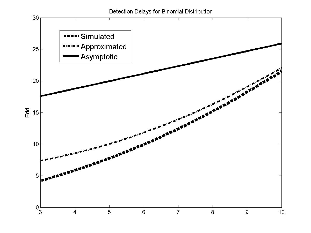
(a) Detection Delay

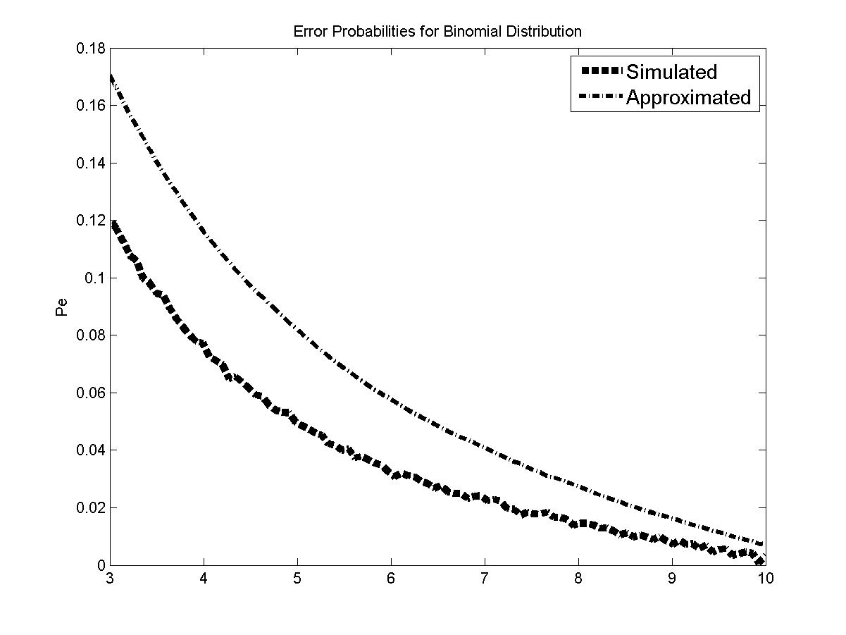
(b) Error Rate

Figure 1: Performance of Newest Algorithm for Binomial Distribution

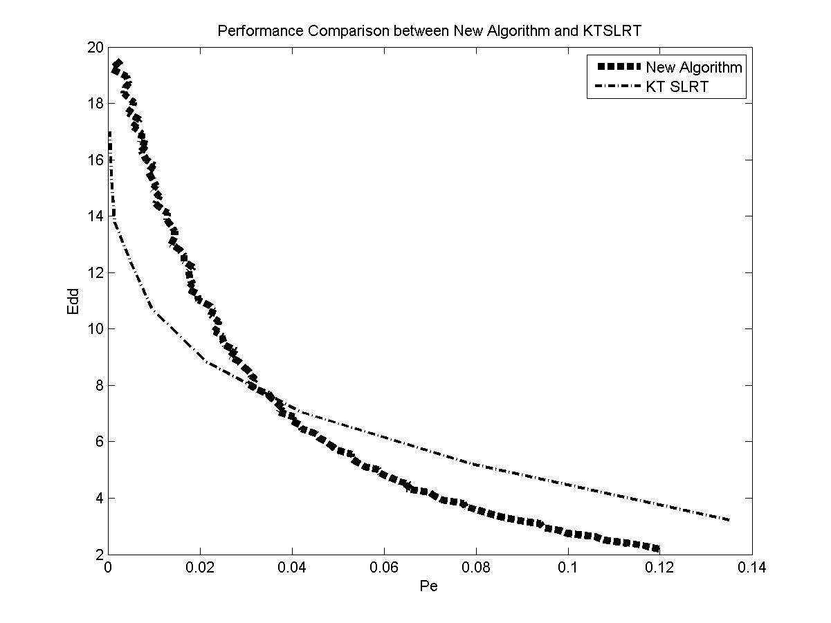
(a) Simulated

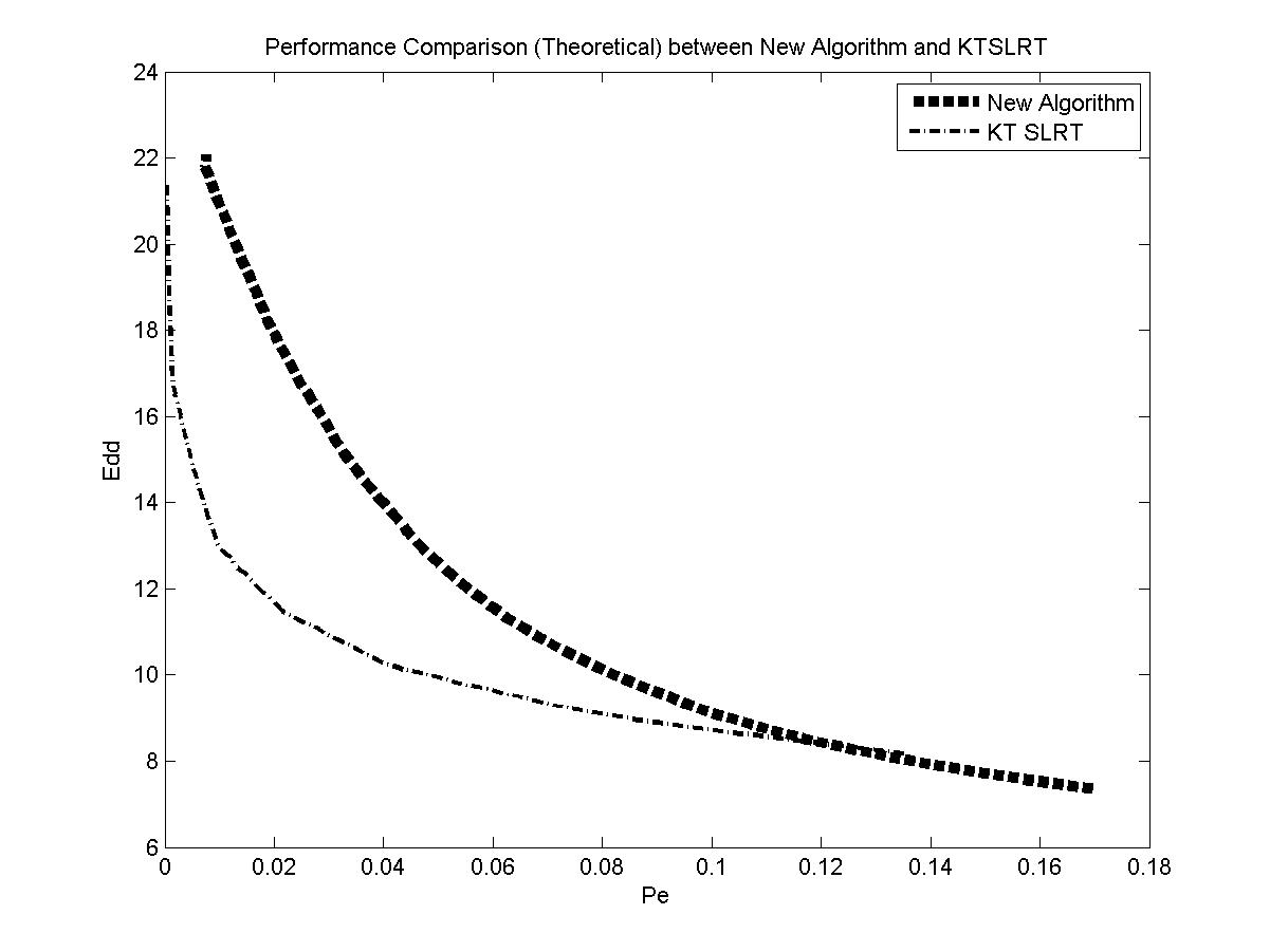
(b) Theoretical

Figure 2: Performance Comparison between Newest Algorithm and KT-SLRT for Binomial Distribution

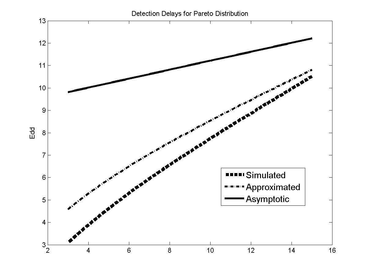
(a) Detection Delay

(b) Error Rate

Figure 3: Performance of Newest Algorithm for Pareto Distribution

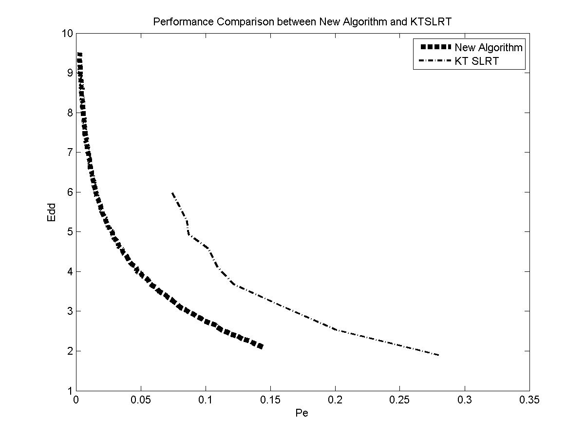
(a) Simulated

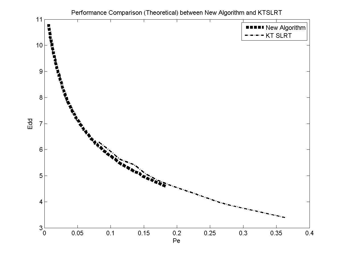
(b) Theoretical

Figure 4: Performance Comparison between Newest Algorithm and KT-SLRT for Pareto Distribution

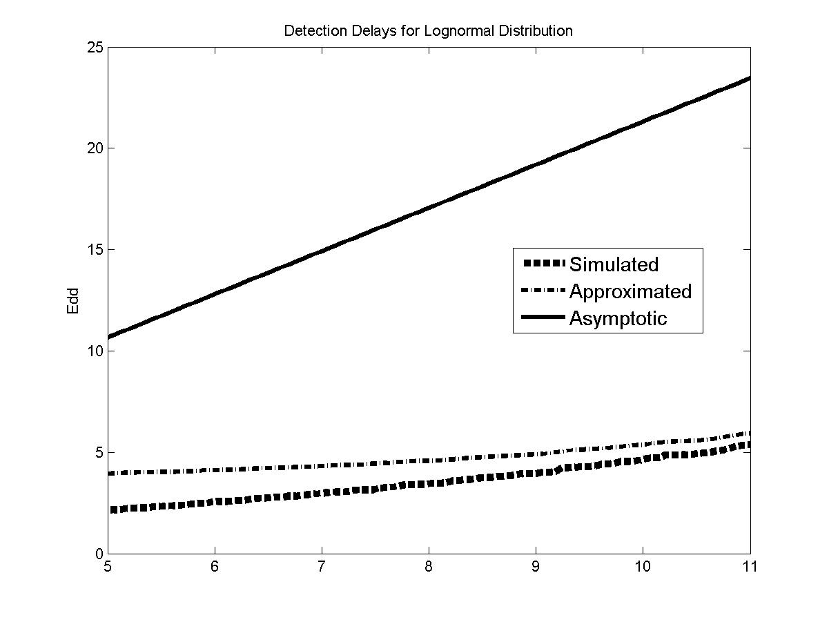
(a) Detection Delay

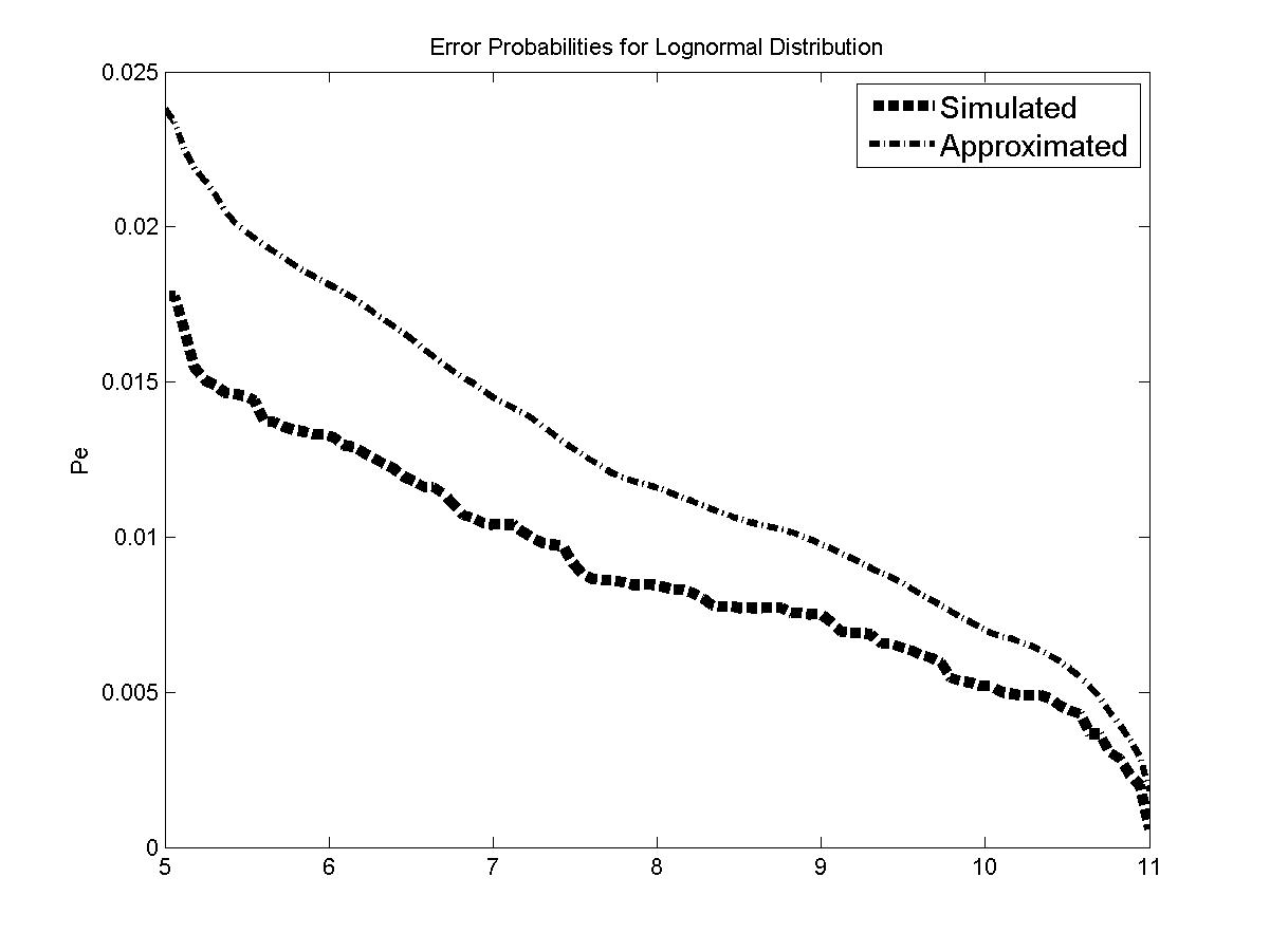
(b) Error Rate

Figure 5: Performance of Newest Algorithm for Lognormal Distribution

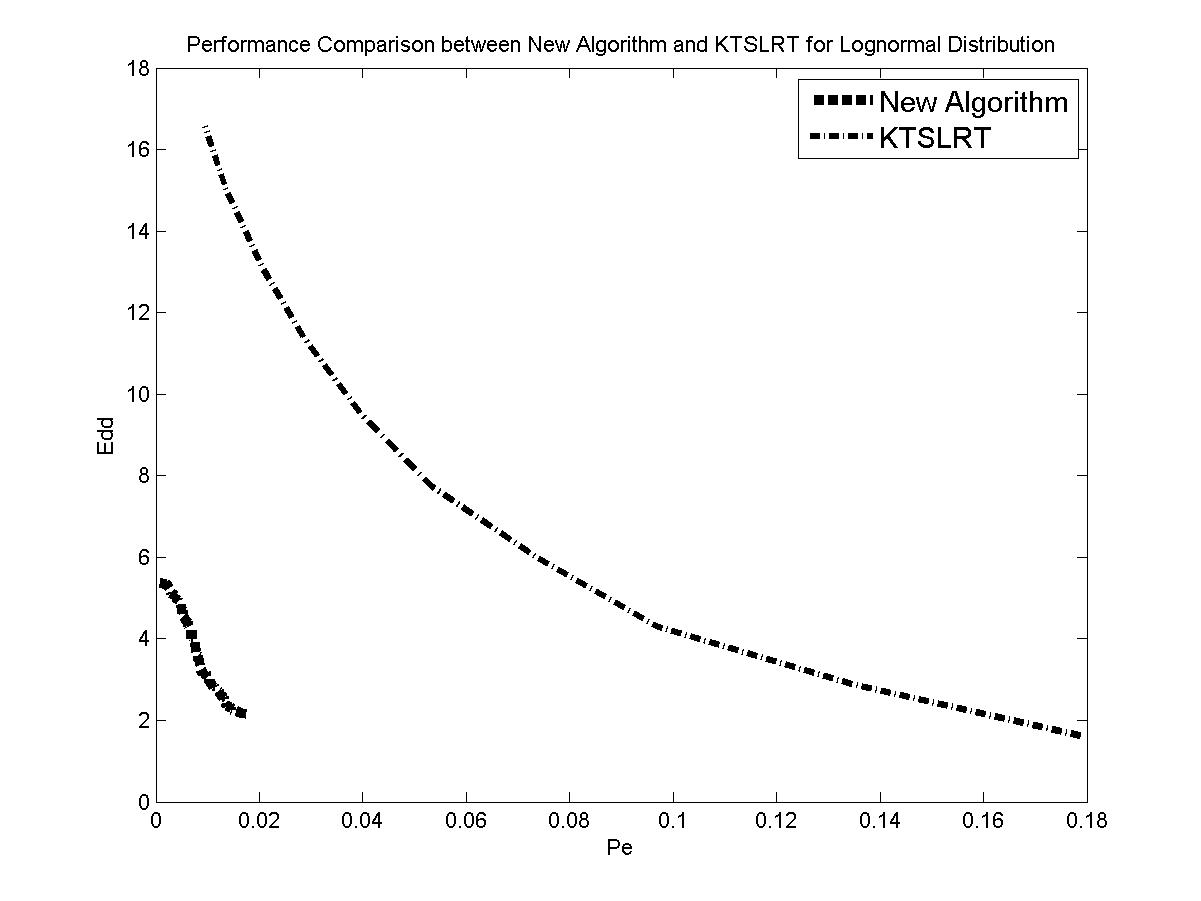
(a) Simulated

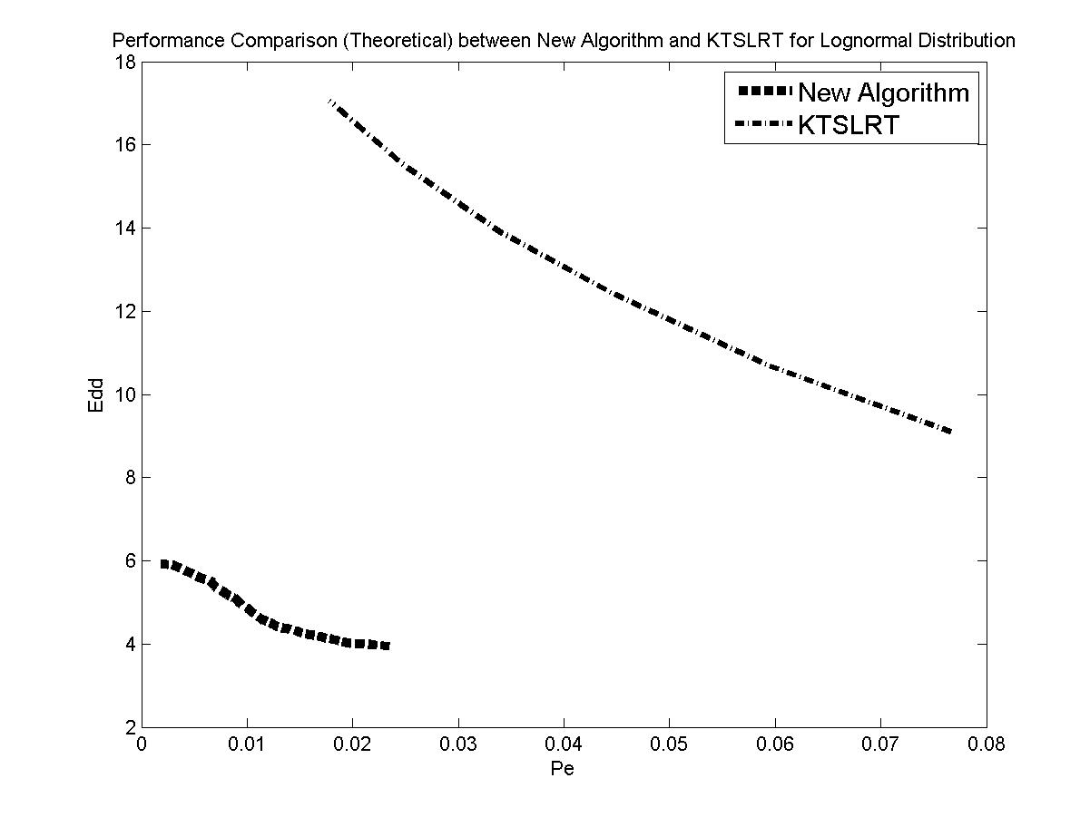
(b) Theoretical

Figure 6: Performance Comparison between Newest Algorithm and KT-SLRT for Lognormal Distribution

(a) Detection Delay

(b) Error Rate

Figure 7: Performance of Newest Algorithm for Gaussian Distribution

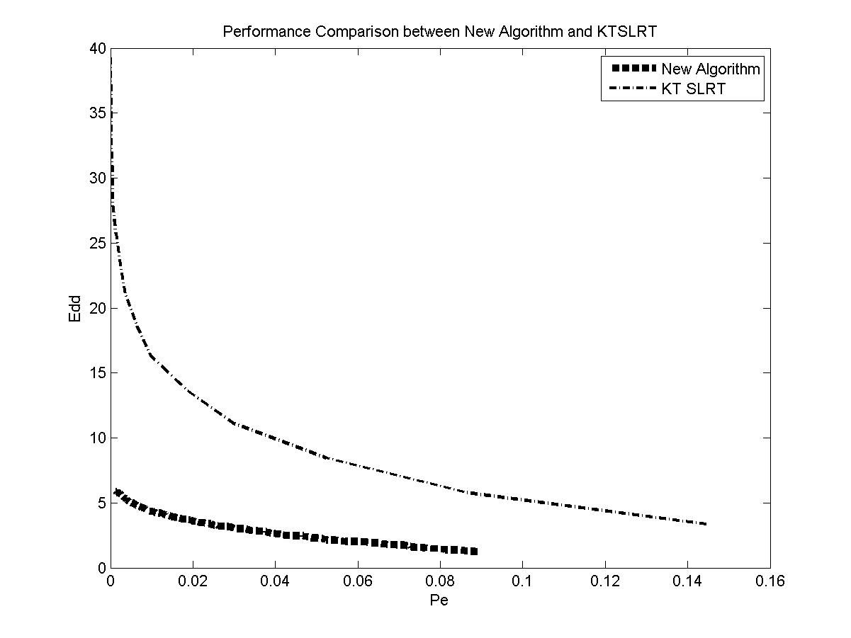
(a) Simulated

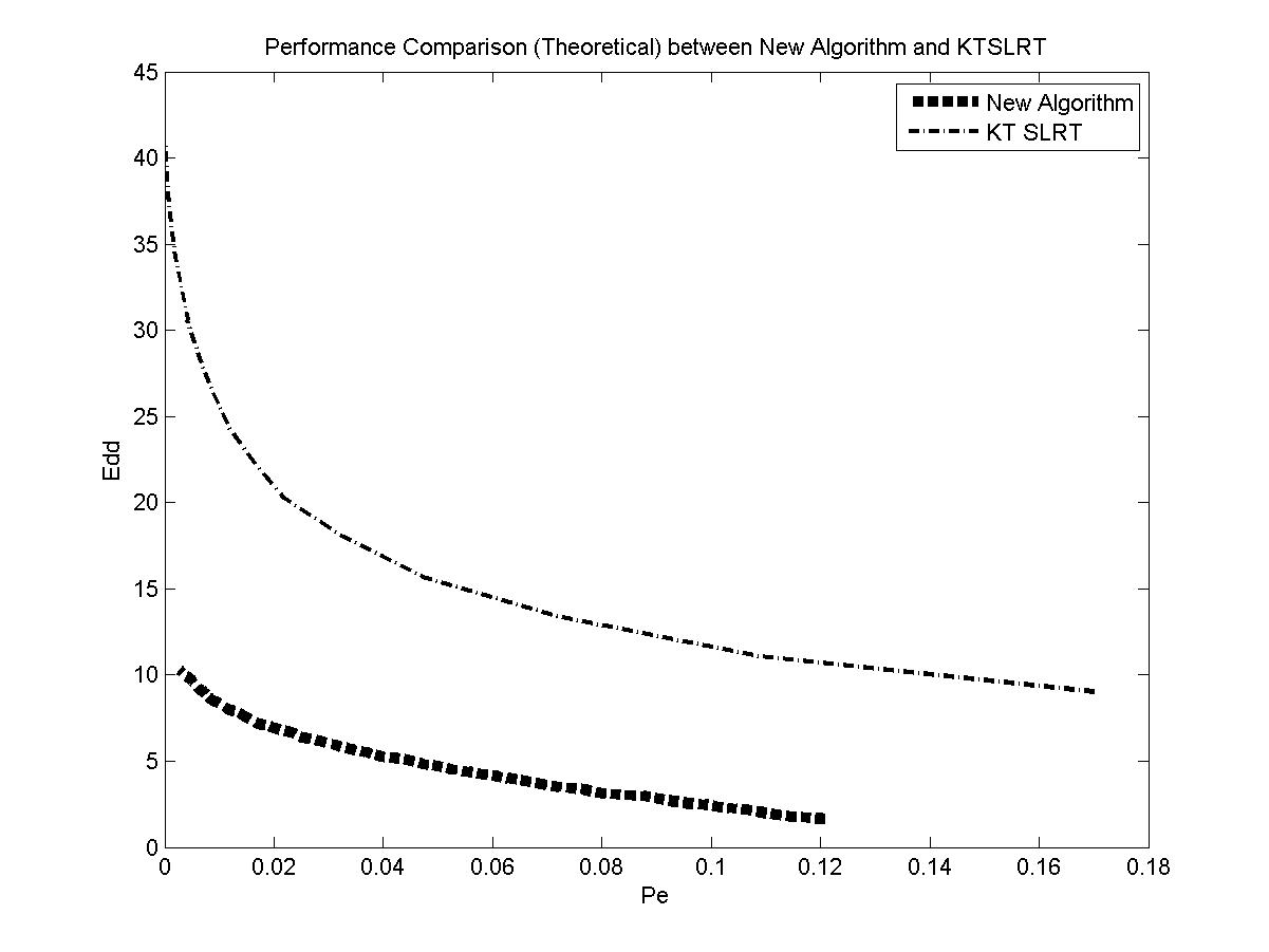
(b) Theoretical

Figure 8: Performance Comparison between Newest Algorithm and KT-SLRT for Gaussian Distribution

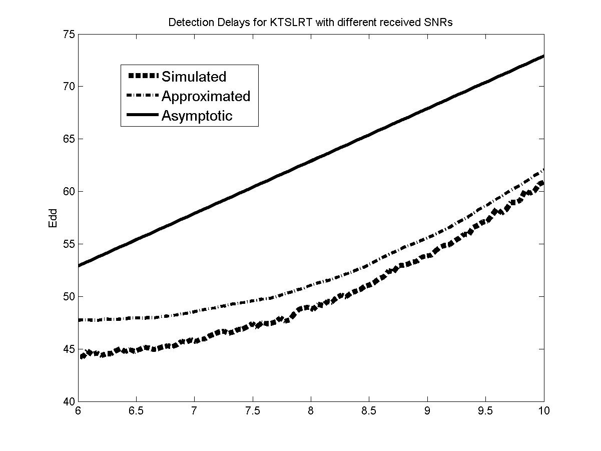
(a) Detection Delay

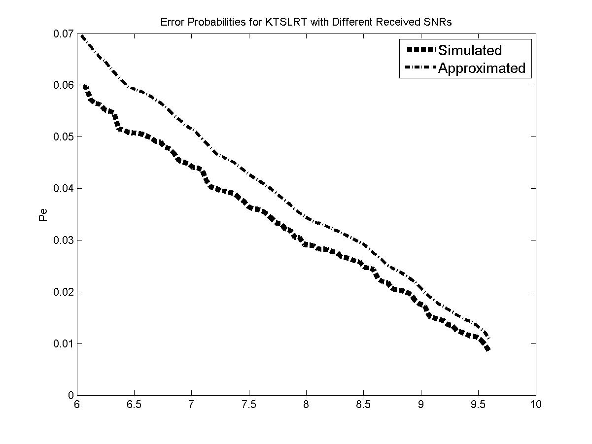
(b) Error Rate

Figure 9: Performance of KTSLRT for Gaussian Distribution with different received SNRs

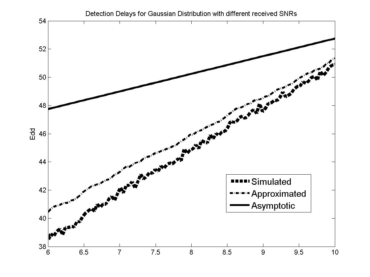
(a) Detection Delay

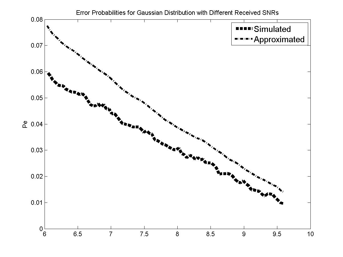
(b) Error Rate

Figure 10: Performance of Newest Algorithm for Gaussian Distribution with different received SNRs

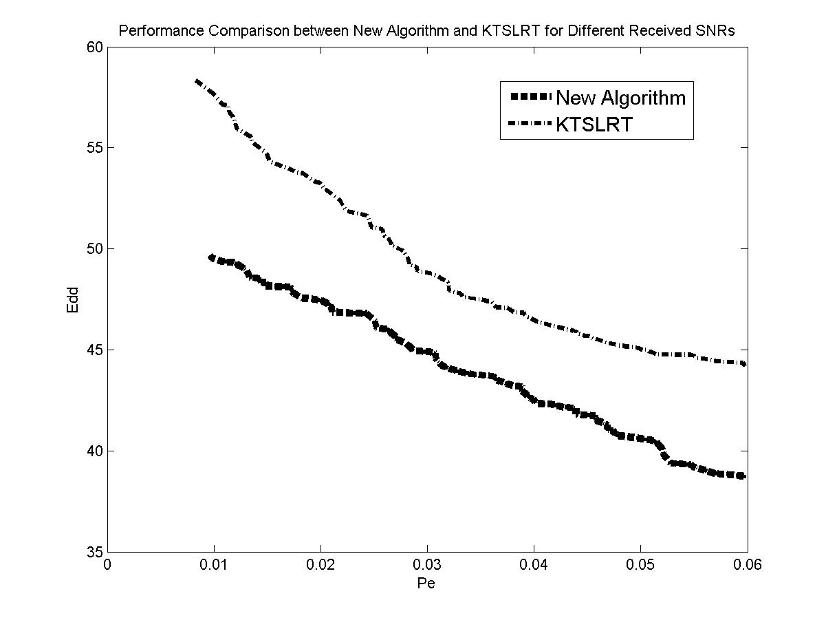
(a) Simulated

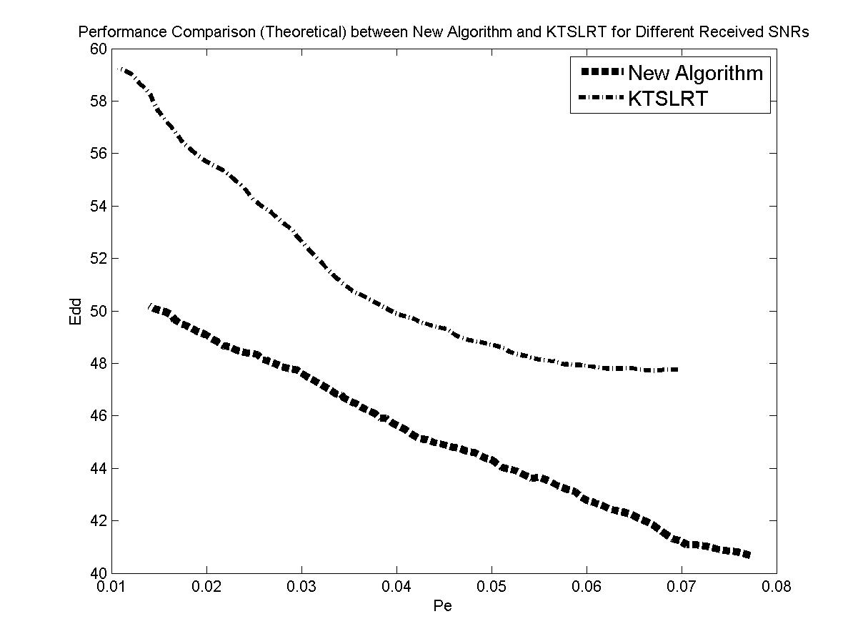
(b) Theoretical

Figure 11: Performance Comparison between Newest Algorithm and KT-SLRT for Gaussian Distribution with different received SNRs

VIII Further Generalizations

Let us now consider a generalization of the problem, in which $P_{0}$ is not exactly known. Specifically, the hypothesis testing problem we now consider is:

$$H_{0}:P\in\{P_{0}^{\prime}:D(P_{0}^{\prime}||P_{0})\leq\gamma\lambda\},\mbox{ for some }0\leq\gamma<1.$$ (1)

$$H_{1}:P\in\{P_{1}^{\prime}:D(P_{1}^{\prime}||P_{0})\geq\lambda\mbox{ and }H(P_{1}^{\prime})>H(P_{0}^{\prime}),$$

for all $P_{0}^{\prime}\in H_{0}\}$
The detection algorithm remains the same except that now we write the test statistic at the local node $l$ as

$$\widetilde{W}_{k,l}=\widetilde{W}_{k-1,l}-\log\hat{P}_{0}(X_{k,l})-H(\hat{P}_{0})-\upsilon\lambda.$$

For good performance we should pick $\hat{P}_{0}$ from the class in (5) and choose $\upsilon$ carefully. We elaborate on this in the following.

Let us try to justify this problem statement from a practical CR standpoint. In a CR setup, $H_{0}$ actually indicates the presence of only noise, while under $H_{1}$, the observatios are signal $+$ noise. Due to electromagnetic interference, the receiver noise can be changing with time ([sahai]). Thus we assume that the noise power $P_{N}$ is bounded as $\sigma_{N,L}^{2}\leq P_{N}\leq\sigma_{N,H}^{2}$. Similarly, let the signal power be bounded as $\sigma_{S,L}^{2}\leq P_{S}\leq\sigma_{S,H}^{2}$. Now we formulate these constraints in the form (5) where we should select appropriate $P_{0}$, $\lambda$ and $\gamma$. We will compute these assuming we are limiting ourselves to Gaussian distributions but will see that these work well in general.

We take, $P_{0}\sim\mathcal{N}(0,\sigma_{0}^{2})$, with $\sigma_{0}$ determined from the given bounds as follows.

Given two Gaussian distributions $Q_{0}$ and $Q_{1}$ with zero mean and variances $\sigma_{0}^{2}$ and $\sigma_{1}^{2}$ respectively,

$D(Q_{1}||Q_{0})=\displaystyle\ln\frac{\sigma_{0}}{\sigma_{1}}+\frac{1}{2}(\frac{\sigma_{1}^{2}}{\sigma_{0}^{2}}-1)$
Let $f(\sigma)\triangleq\displaystyle\ln\frac{\sigma_{0}}{\sigma}+\frac{1}{2}(\frac{\sigma^{2}}{\sigma_{0}^{2}}-1)$. We choose $\sigma_{0}$ such that $f(\sigma_{N,L})=f(\sigma_{N,H})$. This can be achieved for some $\sigma_{0}\in(\sigma_{N,L},\sigma_{N,H})$, since $f$ is convex with a minimum at $\sigma_{0}$. This choice ensures that $P_{0}$ is at some sort of a ”centre” of the class of distributions under consideration in $H_{0}$. We now choose $\gamma\lambda\triangleq f(\sigma_{N,L})=f(\sigma_{N,H})$.

For the class of distributions considered under $H_{1}$,

$$\sigma_{N,L}^{2}+\sigma_{S,L}^{2}\leq E[X^{2}]\leq\sigma_{N,H}^{2}+\sigma_{S,H}^{2}.$$

We take,

$$\lambda\triangleq\displaystyle\inf_{\sigma^{2}\in(\sigma_{N,L}^{2}+\sigma_{S,L}^{2},\sigma_{N,H}^{2}+\sigma_{S,H}^{2})}f(\sigma)=f(\sqrt{\sigma_{N,L}^{2}+\sigma_{S,L}^{2}}).$$

Next we compute $\hat{P}_{0}$. If the $X_{k,l}$ has distribution $P_{i}^{\prime}$ for $i=0,1$, then the drift at the local nodes is $D(P_{0}^{\prime}||\hat{P}_{0})+H(P_{0}^{\prime})-H(\hat{P_{0}})-\upsilon\lambda$ under $H_{0}$, and $D(P_{1}^{\prime}||\hat{P}_{0})+H(P_{1}^{\prime})-H(\hat{P_{0}})-\upsilon\lambda$ under $H_{1}$. This drift is an important parameter in determining the algorithm performance and will decide $\hat{P}_{0}$.

Let $W_{i}$ be the cost of rejecting $H_{i}$ wrongly, and $c$ be the cost of taking each observation. Then, Bayes risk for the test is given ([estimation]) by
$\mathcal{R}_{c}(\delta)=\displaystyle\sum_{i=0}^{1}\pi^{i}[W_{i}P_{i}(\mbox{ reject }H_{i})+cE_{i}(N)]$, where $\pi^{i}$ is the prior probability of $H_{i}$.
Taking the same thresholds as in Section V and using Theorems 5.1 and 5.2,

$\displaystyle\lim_{c\to 0}\frac{\mathcal{R}_{c}(\delta)}{c|\log c|}$

$\leq\frac{\pi^{0}}{L[-D(P_{0}^{\prime}||\hat{P}_{0})-H(P_{0}^{\prime})+H(\hat{P_{0}})+\upsilon\lambda]}(1-\frac{\theta_{0}}{\Delta(\mathcal{A}^{0})})+$
$\frac{\pi^{1}}{L[D(P_{1}^{\prime}||\hat{P}_{0})+H(P_{1}^{\prime})-H(\hat{P_{0}})-\upsilon\lambda]}(1+\frac{\theta_{1}}{\Delta(\mathcal{A}^{1})})$

$$-\frac{\pi^{0}}{\Delta(\mathcal{A}^{0})}+\frac{\pi^{1}}{\Delta(\mathcal{A}^{1})}.$$ (2)

Following a minimax approach, we first maximize the above expression with respect to $P_{0}^{\prime}$ and $P_{1}^{\prime}$, and then minimize the resulting maximal risk w.r.t. $\hat{P}_{0}$ and $\upsilon$. As noted before, we achieve this optimization limiting ourselves to only Gaussian family.

The second term in (6) is maximized when $D(P_{1}^{\prime}||\hat{P}_{0})+h(P_{1}^{\prime})$ is minimized. Let us denote the variance of $\hat{P}_{0}$ by $\Gamma$. Now, the variances of all eligible $P_{1}^{\prime}$s are greater than $\Gamma^{2}$. Hence, $D(P_{1}^{\prime}||\hat{P}_{0})+h(P_{1}^{\prime})$ is minimized when $P_{1}^{\prime}$ has the least possible variance, i.e. $\sigma_{N,L}^{2}+\sigma_{S,L}^{2}$. Using $\mathcal{N}(0,\sigma_{N,L}^{2}+\sigma_{S,L}^{2})$ in place of $P_{1}^{\prime}$, the second term in (6) becomes (after simplification),

$$\frac{(\pi^{1}/L)(1+\frac{\theta_{1}}{\Delta(\mathcal{A}^{1})})}{\frac{1}{2}(\frac{\sigma_{N,L}^{2}+\sigma_{S,L}^{2}}{\Gamma^{2}}-1)-\upsilon\lambda}.$$

Similarly, to maximize the first term in (6), we have to minimize $D(P_{0}^{\prime}||\hat{P}_{0})+H(P_{0}^{\prime})$ w.r.t. $P_{0}^{\prime}$. After this, the first term becomes $\displaystyle\frac{(\pi^{0}/L)(1-\frac{\theta_{0}}{\Delta(\mathcal{A}^{0})})}{\upsilon\lambda-\frac{1}{2}(\frac{\sigma_{N,H}^{2}}{\Gamma^{2}}-1)}$.

$$\mbox{Taking }x\triangleq\displaystyle\frac{1}{\Gamma^{2}},y\triangleq\upsilon\lambda,a=\sigma_{N,H}^{2},b=\sigma_{N,L}^{2}+\sigma_{S,L}^{2},$$

$$A=(\pi^{0}/L)(1-\frac{\theta_{0}}{\Delta(\mathcal{A}^{0})})\mbox{ and }B=(\pi^{1}/L)(1+\frac{\theta_{1}}{\Delta(\mathcal{A}^{1})}),$$ (3)

the non-constant part of the optimized expression (6) can be written as a function of $x$ and $y$ in the form,

$$g(x,y)=\displaystyle\frac{A}{y+\frac{1}{2}-\frac{1}{2}ax}+\frac{B}{\frac{1}{2}bx-y-\frac{1}{2}}.$$

Minimizing this w.r.t. $y$ yields,

$$y_{opt}=\displaystyle\frac{1}{2}\frac{\sqrt{A}(bx-1)+\sqrt{B}(ax-1)}{\sqrt{A}+\sqrt{B}}$$ (4)

Together with this, we can choose $x\in\displaystyle(\frac{1}{\sigma_{N,H}^{2}},\frac{1}{\sigma_{N,L}^{2}})$.

In the following, we demonstrate the advantage of optimizing the above parmeters on the examples considered in Section VI. The bounds on the noise and signal power were chosen in each case such that the distributions specified in Section VI satisfy those constraints. Also, the thresholds were chosen the same as before.

For the following simulations, we have taken
$\Gamma^{2}=\displaystyle\frac{\sigma_{N,L}^{2}+\sigma_{N,H}^{2}}{2}$ and determined $y_{opt}$ in accordance with (8).
For Gaussian distribution, $P_{0}^{\prime}\equiv\mathcal{N}(0,1)$, $P_{1}\equiv\mathcal{N}(0,5)$
For Lognormal distribution, $P_{0}^{\prime}\equiv\log\mathcal{N}(0,3)$, $P_{1}\equiv\log\mathcal{N}(3,3)$
For Pareto distribution, $P_{0}^{\prime}\equiv\mathcal{P}(10,2)$, $P_{1}\equiv\mathcal{P}(3,2)$
We compare the performances in Figs. 8-10. We see that the optimized version performs noticeably better, even for distributions other than Gaussian.

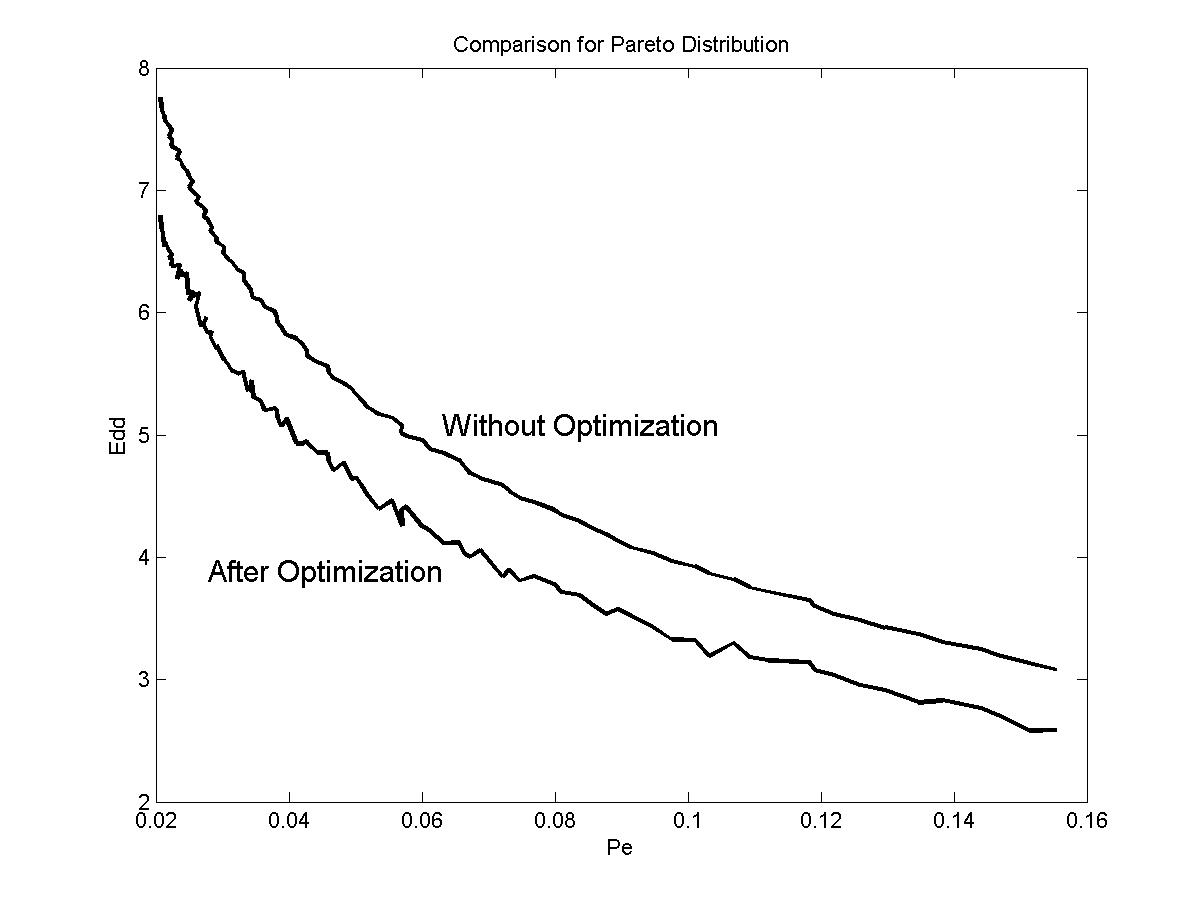
Figure 12: Optimization for Pareto Distribution

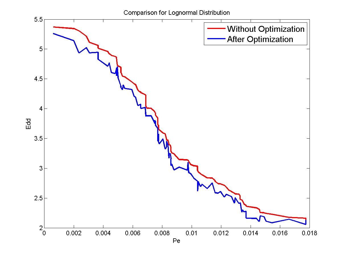
Figure 13: Optimization for Lognormal Distribution

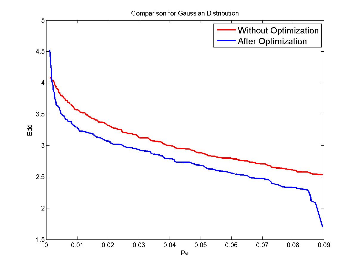
Figure 14: Optimization for Gaussian Distribution

IX Conclusions

We have developed a new distributed sequential algorithm for detection, where under one of the hypotheses, the distribution can belong to a nonparametric family. This can be useful for spectrum sensing in Cognitive Radios. This algorithm is shown to perform better than a previous algorithm which was known to perform well and is also easier to implement. We have also obtained its performance approximately and studied asymptotic performance. The approximations match with the simulations better than the asymptotics. The asymptotics are comparable to SPRT and other known algorithms even though it is in the non-parametric setup.